Discovery of a new INTEGRAL source: IGR J19140$+$0951

IGR J19140$+$0951 (formerly known as IGR J19140$+$098) was discovered with the INTEGRAL satellite in March 2003. We report the details of the discovery, using an improved position for the analysis. We have performed a simultaneous study of the 5–100 keV JEM-X and ISGRI spectra from which we can distinguish two different states. From the results of our analysis we propose that IGR J19140$+$0951 is a persistent Galactic X-ray binary, probably hosting a neutron star although a black hole cannot be completely ruled out.

1 Introduction

The European Space Agency’s INTErnational Gamma-Ray Astrophysical Laboratory (INTEGRAL) was successfully launched on 2002 Oct 17. The INTEGRAL payload consists of two gamma-ray instruments, two X-ray monitors and an optical monitor.
The Imager on Board the INTEGRAL spacecraft (IBIS, Ubertini et al. 2003) is a coded mask instrument designed for high angular resolution (12 arcmin, but source location down to 1 arcmin) imaging in the energy range from $\sim 20$ keV to $\sim 10$ MeV. Its total total field of view is $29^{\circ}\times 29^{\circ}$ for zero response with a uniform sensitivity within the central $\sim 10^{\circ}\times 10^{\circ}$. The INTEGRAL Soft Gamma-Ray Imager (ISGRI, Lebrun et al. 2003) is the top layer of the IBIS detection plane, and covers the energy range from 13 keV to a few hundred keV.
The Joint European X-ray monitor, JEM-X (Lund et al. 2003), consists of two identical coded mask instruments designed for X-ray imaging in the range 3–35 keV with an angular resolution of 3 arcmin and a timing accuracy of 122 $\mu$s. During our observation only the JEM X-2 unit was being used.

Since the start of normal observations in early 2003, INTEGRAL has discovered a number of new transient gamma- and X-ray sources. IGR J19140$+$0951 was discovered in the region tangent to the Sagittarius spiral arm during observations targeted on GRS 1915$+$105 performed from 2003 March 6 through 7 (Hannikainen, Rodriguez & Pottschmidt 2003). The position of the source (Hannikainen et al. 2003) obtained with an early version of the Offline Scientific Analysis software (OSA) was within the error contour of a weak X-ray source EXO 1912+097 (Lu et al. 1996). A ToO performed on IGR J19140$+$0951 with the Rossi X-ray Timing Explorer allowed the absorption column density ${\mathrm{N}}_{\mathrm{H}}$ to be estimated to $\sim 6\times 10^{22}$ cm^-2 (Swank & Markwardt 2003). Recently a (likely orbital) period of 13.55 days has been obtained from re-analysis of the RXTE/All Sky Monitor (Corbet, Hannikainen, Remillard 2004), suggesting a binary nature of the source.
In this Letter we report the details of the discovery of the source with INTEGRAL, study its temporal variability as well as spectral evolution on timescale $\sim 30$ min over this observation. In Sec. 2 we give the details of the data reduction methods that are employed in the course of this analysis. We then present our results in Sec. 3, giving in particular the most accurate position of the source (Cabanac et al. 2004), and discuss our findings in the last part of the letter.

2 Observations and data reduction

The INTEGRAL observation was undertaken using the hexagonal dither pattern (Courvoisier et al. 2003): this consists of a hexagonal pattern around the nominal target location (1 source on-axis pointing, 6 off-source pointings, each 2 degrees apart). The entire duration of a pointing (science window) is 2200 s, but after applying a good time interval correction the effective exposure time is $\sim 1700$ s. The observations were continuous, except for a short slew between each science window.
The JEM X-2 data were reduced using OSA 3.0 software, following the standard procedure explained in the cookbook. This was especially useful for the spectral extraction. In this case we forced the extraction of data products for IGR J19140$+$0951, giving to the software the updated position of the source discussed in this Letter. The resultant spectra were grouped so that each new bin contained a minimum of 60 counts, and systematic uncertainties (P. Kretschmar, priv. comm.) have been applied as follows: 10% between channels 59 and 96 (4$-$7.04 keV), and 2% above channel 97 ($>7.04$ keV).
The IBIS/ISGRI data were reduced using pre-OSA 4.0 version of the software. This new software includes the same core as OSA 3.0 except updated patches for ibis_isgr_energy (v5.1), ibis_isgr_deadtime (v4.2), ii_shadow_build (v1.4), ii_shadow_ubc (v2.7), ii_skyimage (v6.7.2) & ii_spectra_extract (v2.2), which fix many of the OSA3.0 known issues. We made two runs of the software up to the IMA level, i.e. production of images. During the first run we extracted images from individual science windows in two energy ranges (20–40 keV, and 40–80 keV), as well as a mosaic in the same energy range. Figure 1 shows a zoomed IBIS/ISGRI image of the field of the new transient. The standard ISDC catalogue v13 was given as an input, and the software was let free to find the most significant peaks in the images. This provided us with the best position for the source which was used (together with the JEM-X position) to update the entry of IGR J19140$+$0951 in the standard catalogue. This first run was also used to identify the sources clearly seen during our observation (only 7 were detected in the 20–40 keV mosaic). We then created a second catalogue containing only those sources. This second catalogue was given as the input for the second run, and we forced the software to extract the source count rate in every science window at the position of the catalogue. Note that the same process was re-applied in the 20–40 keV and 40–80 keV energy ranges, to obtain the “true” lightcurves of the source. They are shown in Fig. 2.

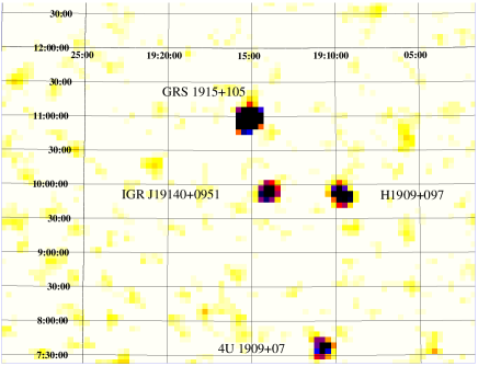
Figure 1: The IBIS/ISGRI 20–30 keV image, showing the new source and three other sources in the field-of-view. GRS 1915$+$105 is bright in this energy range. The image is $\sim 7^{\circ}$ width and $\sim 5^{\circ}.3$ height. North is up and East is to the left. The other sources in the field are dealt with in Molkov et al. (2004)

We then extracted spectra from each science window with the Least Square Method. A preliminary Crab-corrected response matrix rebinned to 16 spectral channels was used in the extraction process and then in the subsequent fitting process. The resultant spectra were further grouped so that each new bin had a minimum of 20 counts, while 5% systematics have been applied to all channels (Goldwurm et al. 2003). The spectra were then fitted in XSPEC v11.3, with a newly available ancillary response file (P. Laurent, priv. comm.). We retained the energy channels between 5 and 25 keV for JEM X-2 and those between 20 and 100 keV for ISGRI.

3 Results

3.1 Refining the position of IGR J19140$+$0951

The source was discovered soon after the observation began (Hannikainen et al. 2003) in near real time data, using an early version of the software (OSA1.0). It was first spontaneously detected in science window 3 at a level of $\sim 3$ cts/s in the 20–40 keV (26 mCrab), and reached a level of $\sim 6$ cts/s ($\sim 52$ mCrab) in the following science window. In the latter it was even detected above 40 keV, at a level of $2.4$ cts/s ($\sim 35$ mCrab). The source position had been obtained using only those science windows where the source was spontaneously detected by the software in ISGRI. Concerning the JEM X-2 data reduction, we used the “JEM-X offline software” (Lund et al. 2004) to constrain with more accuracy the new position.
We have refined the position using both JEM X-2 and ISGRI data. IGR J19140$+$0951 is clearly detected in nine independent science windows of the whole observing programme. Among them, the source was detected in two energy bands (8.4–14 keV and 14–35 keV) three times, thus we used those 12 independent detections to derive a best (JEM-X) weighted mean position of (J2000, errors at 1.64 $\sigma$):
$\mathrm{RA}=19^{\mathrm{h}}14^{\mathrm{m}}01^{\mathrm{s}}\pm 9s$ and $\mathrm{Dec}=9^{\circ}53^{\prime}21^{\prime\prime}\pm 1.3^{\prime}$.
In the same way IGR J19140+0951 is clearly detected in IBIS/ISGRI mosaics (Fig. 1) in both energy ranges. We can derive a best (ISGRI) position of (J2000):
$\mathrm{RA}=19^{\mathrm{h}}14^{\mathrm{m}}02.7^{\mathrm{s}}\pm 2^{\prime}$ and $\mathrm{Dec}=9^{\circ}53^{\prime}13^{\prime\prime}\pm 2^{\prime}$ (all errors are at the 90% confidence level, see e.g. Gros et al. 2003). From these two independent data sets we can estimate the most accurate (weighted mean) position of the source of :
$\mathrm{RA}=19^{\mathrm{h}}14^{\mathrm{m}}02^{\mathrm{s}}$ and $\mathrm{Dec}=9^{\circ}53.3^{\prime}$ (1.3^′ error at 90%, Cabanac et al. 2004). The source is 5.2^′ away from EXO 1912$+$097 (Lu et al. 1996). As the EXOSAT error box is 6^′ it is possible that the EXOSAT detection represents an earlier outburst of the source seen by INTEGRAL. The EXOSAT source was discovered using the demodulation technique (Lu et al. 1996), but besides this detection nothing is known about this source.

3.2 Temporal variability

Figure 2 shows the 20–40 keV and 40–80 keV lightcurves during Revolution 48. It is immediately apparent that the source is variable on the timescale of 2200 seconds (typical duration of a science window) during the observation. In the 20–40 keV range the source is detected at a flux higher than the 3-$\sigma$ limit of $9-10$ mCrab in 70$\%$ of the science windows. It is found at a level of $\sim 20$ mCrab in the 20–40 keV range 50$\%$ of the time, and undergoes flares on rather short timescales up to a level of 70 mCrab on one occasion. The flares in the 20–40 keV range are accompanied by flaring also in the 40–80 keV range, reaching levels of $\sim$38 mCrab.

Figure 2: The 20–40 keV (top) and 40–80 keV (bottom) ISGRI lightcurves. Each symbol represents a science window. The 3-sigma upper limits are denoted with an arrow. The dashed line in the upper panel indicates the 20 mCrab level.

3.3 Spectral analysis

To begin our spectral analysis, we extracted spectra from each one of the 46 science windows from both JEM X-2 and ISGRI, as explained in Sec. 2. Based on the lightcurve shown in Fig. 2, we selected only the science windows where IGR J19140$+$0951 is clearly detected at a significance level greater than $3\sigma$ in the 20–40 keV range. We then fitted the JEM X-2 and ISGRI spectra simultaneously, with a simple model consisting of an absorbed power law. The value of ${\mathrm{N}}_{\mathrm{H}}$, was frozen to the value obtained with RXTE (Swank & Markwardt 2003), i.e. $6\times 10^{22}$ cm^-2, since the useful energy range of JEM X-2 does not allow us to obtain a better constraint on this parameter. We did a first run with a multiplicative constant to account for cross-calibration of the instruments, but it was found to be very close to 1 in each spectrum. Therefore, in a second run no such constant was included. Fig. 3 shows the results obtained for the science windows for which a good fit was achieved. This excludes three science windows.

Figure 3: The powerlaw photon index for the science windows for which a good fit was obtained. The horizontal dashed line shows the $\Gamma=2.5$ level.

To increase our statistics, we further averaged all the spectra from the science windows in which IGR J19140$+$0951 is found at a flux up to $\sim$20 mCrab between 20 and 40 keV (Fig. 2; hereafter this spectrum is referred to as “faint”). In addition we also averaged together all the spectra where the source was found to be at a level of $>$20 mCrab (referred to as “bright”). The ftool mathpha was used to compute the true weighted average spectrum (K. Ebisawa, priv. comm.). Fig. 4 shows the spectra obtained after the averaging processes. Although a simple model fits the single spectra well, it gives a relatively poor reduced chi square for the the average spectra (1.55 for 65 dof in the case of the “faint” spectrum, and 1.48 for 73 dof, in the case of the “bright” spectrum).

Figure 4: The faint (left) and bright (right) spectra with the best-fit model superimposed, a blackbody $+$ powerlaw for the faint spectrum and comptt for the bright spectrum.

Faint spectrum. Adding a blackbody to the simple powerlaw improves the fit to a reduced $\chi^{2}=1.19$ (63 dof). An F-test indicates that the blackbody component is required at a level greater than 99.99%. The temperature is kT=$1.27^{+0.07}_{-0.08}$ keV and $\Gamma=2.39\pm 0.11$. The 2–20 keV (20–100 keV) unabsorbed flux is 9.80$\times 10^{-10}$ erg s^-1 cm^-2 (1.96$\times 10^{-10}$ erg s^-1 cm^-2). Fig. 4 (left) shows the faint spectrum with the best-fit model.

Bright spectrum. The blackbody is only marginally required with an F-test probability of 92%. However, adding a high energy cutoff to the simple powerlaw improved the fit to a reduced $\chi^{2}=0.93$ which leads to an F-test probability of $>$99.99%. The powerlaw photon index is 2.03$\pm 0.04$. The cutoff energy is 49$\pm 3$ keV and the folding energy is 16${}^{+4}_{-7}$ keV. Since the cutoff in a powerlaw is attributed to thermal Comptonization we also fitted the bright spectrum with comptt (Fig. 4, right). Given the energy range, the temperature of the input photons was frozen to 0.5 keV. The electron temperature is 15.1${}^{+2.5}_{-1.6}$ keV and the optical depth of the plasma is 2.1${}^{+0.2}_{-0.3}$. The reduced $\chi^{2}$ is 1.07 for 71 dof. The 2–20 keV (20–100 keV) unabsorbed flux is 1.01$\times 10^{-9}$ erg s^-1 cm^-2 (5.39$\times 10^{-10}$ erg s^-1 cm^-2). Adding a blackbody and fixing its parameters to those of the faint spectrum leads to a very bad fit, ruling out a constant blackbody emission.

4 Discussion

The refined position has allowed us to perform an improved analysis of IGR J19140$+$0951 using both JEM-X and ISGRI data. In particular, this has enabled us to obtain the true ISGRI lightcurve on a timescale of $\sim$2000 s as well as individual JEM X-2 and ISGRI spectra. The ISGRI lightcurve shows that the source is variable on the timescale of a science window, so this would imply a maximum size of the emitting region of $\sim 7\times 10^{13}$ cm, i.e. $\sim$4 AU. This, together with the newly-discovered period of 13.55 days, implies the Galactic origin of IGR J19140$+$0951. It is interesting to note that throughout the 100 ksec observation, the source went from being undetectable in the INTEGRAL instruments to a level of 80 mCrab in the 20–40 keV ISGRI range. The variations appear to be not only related to a global change in luminosity but rather reflect changes in the emitting media – for example the appearance and possible disappearance of a blackbody component in the spectra. This is reminiscent of X-ray binaries (e.g. Tanaka & Shibazaki 1996) and the newly-discovered period of 13.55 days (Corbet et al. 2004) strongly points to the binary nature of IGR J19140$+$0951.
The spectral parameters obtained for this object could be consistent with both types for the primary, i.e. either a neutron star or a black hole. In fact, although neutron stars usually have a lower energy cutoff in their spectra, some black holes can show a cutoff as low as 30 keV (e.g. XTE J1550$-$564, Rodriguez et al. 2003). However, in the latter the low energy of the cutoff is accompanied by the very bright emission of soft X-rays (close to 1 Crab in the 1–10 keV range) which is not the case here. In addition, the main difference between a neutron star and a black hole in thermal Comptonization is related to the temperature of the electrons (Barret 2001). In the first phenomenological model we used, it is usually admitted that it is more the folding energy which is close to the electron temperature rather than the cutoff energy. In that case, IGR J19140$+$0951 manifests the expected difference for a neutron star compared to a black hole such as XTE J1550$-$564. This and the persistence of the source would point to a neutron star rather than a black hole. However, a black hole cannot be dismissed since the variations of the photon index (Fig. 3) are similar to those seen in GRS 1915$+$105 (e.g. Markwardt et al. 1999).
The high energy tail would represent the Comptonization of the soft photons on relativistic electrons. And indeed, the averaged bright spectrum is well fitted with a thermal Comptonization model. In addition to a variation in the blackbody, or thermal, component, the variations may also indicate transitions between thermal Comptonization and non-thermal or hybrid thermal-non-thermal Comptonization. The quality of our data does not allow us to answer more precisely these points; a longer accumulation of data in time is currently underway with the aim to increase the statistics at especially the higher energies which in turn will allow us to address this question and the true nature of the compact object.
Further analysis of this source will be deferred to a later paper which will include the remaining INTEGRAL observations from both the Open Time programme and the Galactic Plane Scans of the Core Programme, plus multiwavelength coverage including e.g. the Nordic Optical Telescope and the VLA.

- (1) Barret, D. 2001, Adv. Space Res., 28, 307
- (2) Cabanac, C., Rodriguez, J., Hannikainen, D., et al. 2004, ATel 272
- (3) Corbet, R.H.D., Hannikainen, D.C., Remillard, R. 2004 ATel 269
- (4) Courvoisier, T.J.-L., Walter, R., Beckmann, V., et al. 2003, A&A, 411, L53
- (5) Goldwurm, A., David, P., Foschini, L., et al. 2003, A&A, 411, L223
- (6) Gros, A., Goldwurm, A., Cadolle-Bel, M., et al. 2003, A&A, 411, L179.
- (7) Hannikainen, D.C., Rodriguez, J. & Pottschmidt, K. 2003, IAUC 8088
- (8) Hannikainen, D.C., Vilhu, O., Rodriguez, J., et al. 2003, A&A, 411, L415
- (9) Lebrun, F., Leray, J.-P., Lavocat, P. et al. 2003, A&A, 411, L141
- (10) Lu, F.J., Li, T.P., Sun, X.J., Wu, M. & Page, C. G. 1996, A&AS, 115, L395
- (11) Lund, N., Budtz-Jørgensen, C., Westergaard, N.J., et al. 2003, A&A, 411, L231
- (12) Lund, N. et al. 2004, Proceedings of the 5th INTEGRAL Workshop
- (13) Markwardt, C.B., Swank, J.H. & Taam, R.E. 1999, ApJ, 513, L37
- (14) Rodriguez, J., Corbel, S. & Tomsick, J.A. 2003, ApJ, 595, 1032
- (15) Swank, J.H. & Markwardt, C.B. 2003, ATel 128.
- (16) Tanaka, Y. & Shibazaki, N. 1996, ARA&A, 34, 607
- (17) Ubertini, P., Lebrun, F., Di Cocco, G., et al. 2003, A&A, 411, L131