Quantum cosmological effects from the high redshift supernova observations

Abstract

Subject of this contribution is to demonstrate that the observed faintness of the supernovae at the high redshift can be considered as a manifestation of quantum effects at cosmological scales. We show that observed redshift distribution of coordinate distances to the type Ia supernovae can be explained by the local manifestations of quantum fluctuations of the cosmological scale factor about its average value. These fluctuations can arise in the early universe, grow with time, and produce observed accelerating or decelerating expansions of space subdomains containing separate supernovae with high redshift whereas the universe as a whole expands at a steady rate.

Contents

1. Introduction.

   • Arguments in favour of the quantization of gravity

2. Observations

   • Dark matter and dark energy problem

   • The rate of expansion

3. Quantum model

   • Quantization

   • Boundary conditions and solutions

   • The universe in the state with large quantum numbers

4. Link to the physical data

   • Main cosmological parameters

   • Coordinate distance to source

   • Quantum fluctuations of scale factor

   • Dark matter and dark energy prediction

1 Introduction

Quantum cosmology is the application of quantum theory to the universe as a whole. Since the dominating interaction in the cosmological realm (on the largest scales) is gravity the extrapolation of quantum theory to the whole universe immediately has to address the problem of quantizing the gravitational field (e.g. [Kiefer 1999]). At first glance such an attempt seems surprising since one is used to apply quantum theory to microscopic systems. Nevertheless one can put forward many arguments in favour of the quantization of gravity:

• Unification (as a logical necessity and to avoid inconsistences). All particles are the sources of the gravitational field. If their gravitational fields were really classical, then measuring all the components of these fields simultaneously it would be possible to determine the coordinates and velocities of the particles at once, so that uncertainty principle will be violated. Since the gravitational field is coupled to all other fields, it would be appear strange, and even inconsistent, to have a drastically different framework for this one field.

• Singularity theorems of general relativity. Under very general conditions, the occurrence of a singularity (where the theory breaks down) is unavoidable. Therefore a more fundamental theory is needed. It is expected that a quantum theory of gravity will be such a fundamental theory.

• Initial conditions in cosmology. Since the singularity theorems predict the existence of an initial state with infinite energy density which cannot be described by general relativity, a quantum theory should supply a classical theory of gravity with appropriate initial conditions.

• Field-theory speculations. It is believed that gravity can play the role of a regulator which can automatically eliminate the divergences in ordinary quantum field theory.

• Experiment-theory concordance. A situation in theoretical physics is reflected in the diagram [Isham 1995]:

  $$theory\ \longleftrightarrow\ concepts\ \longleftrightarrow\ facts$$

  in which the theoretical components are linked to the physical data. In the case of quantum gravity it was accepted that the data which can be unambiguously interpreted as a result of quantum effects are absent, so that the diagram is shortened

  $$theory\ \longleftrightarrow\ concepts.$$

  This opinion originates from the fact that the Planck length $l_{Pl}=\sqrt{\frac{\hbar G}{c^{3}}}\simeq 10^{-33}$ cm is extremely small and lies beyond the range of laboratory-based experiments. But it should be noticed that quantum effects are not a priori restricted to certain scales. Rather the process of decoherence [Kiefer 1999] through the environment can explain why quantum effects are negligible or important for the object under consideration.

  In the present contribution we show that the original diagram can be restored if one will consider the whole universe as a laboratory and take into consideration the new astrophysical data from supernovae type Ia observations, CMB anisotropy measurements (WMAP and others), HST key project, which have tremendously increased in volume during the last decade.

2 Observations

2.1 Dark matter and dark energy problem

Observations indicate that overwhelming majority (about 96%) of matter/energy in the universe is in unknown form. The observed mass of stars gives the following values

$$\Omega_{stars}\simeq 0.005\quad\cite[cite]{[\@@bibref{}{Cole et al. 2001}{}{}]},$$

$$\Omega_{stars}\simeq 0.003^{+0.001}_{-0.002}\quad\cite[cite]{[\@@bibref{}{Salucci Persic 1999}{}{}]}$$

for the density of visible (optically bright) baryons. Observations of the cosmic microwave background radiation (CMB) and abundances of the light elements in the universe suggest that the total density of baryons is about 4 % of the total energy density (e.g. [Fukugita & Peebles 2004])

$$\Omega_{B}\simeq 0.04,\qquad\qquad\Omega_{B}/\Omega_{stars}\sim O(10).$$

This value is one order greater than the observed mass of stars. It means that most of baryonic matter today is not contained in stars and is invisible (dark).

The CMB anisotropy measurements allow to determine the total energy density $\Omega_{tot}$ and the matter component $\Omega_{M}$. The recent data give the strong evidence that the present-day universe is spatially flat (or very close to it):

$$\Omega_{tot}\simeq 1$$

[de Bernardis et al. 2000], [Netterfield et al. 2002], [Pryke et al. 2002],
[Sievers et al. 2003], [Spergel et al. 2003] and the mean matter density equals about 30 % of the total energy density. The independent information about the mean matter density $\Omega_{M}$ extracted from the high redshift supernovae Ia data on the assumption that the universe is spatially flat gives the close values:

$$\Omega_{M}=0.29^{+0.05}_{-0.03}\quad\cite[cite]{[\@@bibref{}{Riess et al. 2004}{}{}]}.$$

The discrepancies between the matter density $\Omega_{M}$ and the density of baryons $\Omega_{B}$ on the one hand and the total energy density $\Omega_{tot}$ and the matter density $\Omega_{M}$ on the other hand are signs that there must exist non-baryonic dark matter with the density

$$\Omega_{DM}\simeq 0.25,$$

and some mysterious cosmic substance (so-called dark energy) with the density

$$\Omega_{X}\simeq 0.71.$$

The origin and composition of both dark matter and dark energy are unknown.

Dark matter manifests itself in the universe through the gravitational interaction. Its presence allows to explain rotation curves for galaxies and large-scale structure of the universe in the models with standard assumption of adiabatic density perturbations. As regards dark energy it is worth mentioning that its expected properties are unusual. It is unobservable (in no way could it be detected in galaxies) and spatially homogeneous.

2.2 The rate of expansion

The observed faintness of the type Ia supernovae (SNe) at the high redshift attracts cosmologists’ attention in connection with the hypothesis of an accelerating expansion of the present-day universe proposed for its explanation. Such a conclusion assumes that dimming of the supernovae is hardly caused by physical phenomena non-related to overall expansion of the universe as a whole, such as unexpected luminosity evolution, effects of contaminant gray intergalactic dust, gravitational lensing, and others (e.g. [Tonry et al. 2003]).

Furthermore it is supposed that matter component of energy density in the universe $\rho_{M}$, which includes visible and invisible (dark) baryons and dark matter, varies with the expansion of the universe as $a^{-3}$ (that is it has practically vanishing pressure), where $a$ is a cosmological scale factor,

$$\rho_{M}\sim a^{-3}\quad(p_{M}\approx 0),$$

while dark energy is described by the following equation of state

$$p_{X}=w_{X}\rho_{X},\quad\mbox{where}\ -1\leq w_{X}\leq-\frac{1}{3}.$$

Parameter $w_{X}$ can be constant, as e.g. in the models with the cosmological constant ($\Lambda$CDM-models), or may vary with time as in the rolling scalar field scenario (models with quintessence).

Even if regarding baryon component one can assume that the pressure of baryons may be neglected due to their relative small amount in the universe, for dark matter (whose nature and properties can be extracted only from its gravitational action on ordinary matter) such a dependence on the scale factor may not hold in the universe taken as a whole (in contrast to local manifestations, for example in large-scale structure formation). Since the contribution from all baryons into the total energy density does not exceed 4 % the evolution of the universe as a whole is determined mainly by dark matter and dark energy.

Subject of this contribution is to demonstrate that the observed dimming of the supernovae at the high redshift can be considered as a manifestation of quantum effects at cosmological scales.

3 Quantum model

3.1 Quantization

Just as in ordinary quantum nonrelativistic and relativistic theories one can assume that the problem of evolution and properties of the universe as a whole in quantum cosmology should be reduced to the solution of the functional partial differential equation determining the eigenvalues and the eigenstates of some hamiltonian-like operator (in space of generalized variables, whose roles are played by the metric tensor components and matter fields).

For simplicity we restrict our study to the case of minimal coupling between geometry and the matter. Considering that scalar fields play a fundamental role both in quantum field theory and in the cosmology of the early universe we assume that, originally, the universe is filled with matter in the form of a scalar field $\phi$ with some potential energy density $V(\phi)$.

Let us consider homogeneous and isotropic universe with positive spatial curvature. Assuming that the scalar field $\phi$ is uniform and the geometry is defined by the Robertson-Walker metric, we represent the action functional in the conventional form

$$S=\int d\eta\,\left[\pi_{a}\,\partial_{\eta}a+\pi_{\phi}\,\partial_{\eta}\phi-\mbox{H}\right].$$ (1)

Here $\eta$ is the time parameter (that is related to the synchronous proper time $t$ by the differential equation $dt=N\,a\,d\eta$), $a(\eta)$ is a scale factor; $\pi_{a}$ and $\pi_{\phi}$ are the momenta canonically conjugate with the variables $a$ and $\phi$, respectively. The Hamiltonian H is following

$$\mbox{H}=\frac{1}{2}\,N\,\left[-\,\pi_{a}^{2}+\frac{2}{a^{2}}\,\pi_{\phi}^{2}-a^{2}+a^{4}\,V(\phi)\right]\equiv N\,{\cal R},$$ (2)

where $N(\eta)$ is a function that specifies the time-reference scale. Here and below we use the modified Planck units:

$$l_{P}=\sqrt{2G\hbar/(3\pi c^{3})}=0.74\times 10^{-33}\ \mbox{cm},$$

$$\rho_{P}=3c^{4}/(8\pi Gl_{P}^{2})=1.63\times 10^{117}\ \mbox{GeV cm}^{-3}.$$

The function $N$ plays the role of a Lagrange multiplier, and the variation with respect to $N$ leads to the constraint equation

$$\delta S/\delta N=0\quad\Rightarrow\quad{\cal R}=0.$$

The structure of the constraint is such that true dynamical degrees of freedom cannot be singled out explicitly. In the model being considered, this difficulty is reflected in that the choice of the time variable is ambiguous (so called problem of time). For the choice of the time coordinate to be unambiguous, the model must be supplemented with a coordinate condition. When the coordinate condition is added to the field equations, their solution can be found for chosen time variable. However, this method of removing ambiguities in specifying the time variable does not solve the problem of a quantum description.

Therefore we shall use another approach and remove the above ambiguity with the aid of a coordinate condition imposed prior to varying the action functional. The invariance of action is restored by parametrizing the action. This approach formally agrees with the procedure of transformation from the Wheeler-DeWitt equation to a functional Schrödinger equation (from the Arnowitt, Deser and Misner to the Kuchař description) widely discussed in literature (e.g. [Kuchař & Torre 1991], [Ambrus & Hájíček 2001]).

We will choose the coordinate condition in the form [Kuzmichev 1998], [Kuzmichev 1999], [Kuzmichev & Kuzmichev 2002]

$$g^{00}\left(\partial_{\eta}T\right)^{2}=\frac{1}{a^{2}}\,,\quad\mbox{or}\quad\partial_{\eta}T=N,$$ (3)

where $T$ is the privileged time coordinate, and include it in the action functional with the aid of a Lagrange multiplier $P$

$$S=\int\!d\eta\,\left[\,\pi_{a}\,\partial_{\eta}a+\pi_{\phi}\,\partial_{\eta}\phi+P\,\partial_{\eta}T-{\cal H}\,\right],$$ (4)

where

$${\cal H}=N\,[\,P+{\cal R}\,]$$ (5)

is the new Hamiltonian. The constraint equation reduces to the form

$$P+{\cal R}=0.$$ (6)

Parameter $T$ can be used as an independent variable for the description of the evolution of the universe.

In quantum theory, the constraint equation comes to be a constraint on the wave function that describes the universe filled with a scalar field and radiation. The time-dependent equation has a following form

$$i\,\partial_{T}\Psi=\hat{\mathcal{H}}\Psi,$$ (7)

with a Hamiltonian-like operator

$$\hat{\mathcal{H}}=\frac{1}{2}\left(\partial_{a}^{2}-\frac{2}{a^{2}}\,\partial_{\phi}^{2}-a^{2}+a^{4}V(\phi)\right).$$ (8)

The wavefunction $\Psi$ depends on the cosmological scale factor $a$, scalar field $\phi$, and time coordinate $T$. One can introduce, at least formally, a positive definite scalar product $\langle\Psi|\Psi\rangle<\infty$ and specify the norm of a state. This makes it possible to define a Hilbert space of physical states and to construct quantum mechanics for model of the universe being considered.

Eq. (7) allows a particular solution with separable variables

$$\Psi=\mbox{e}^{\frac{i}{2}ET}\psi_{E},$$ (9)

where the function $\psi_{E}$ is given in $(a,\phi)$-space of two variables and satisfies the time-independent equation

$$\left(-\,\partial_{a}^{2}+a^{2}-a^{4}\hat{\rho}_{\phi}-E\right)\psi_{E}=0.$$ (10)

Here the operator

$$\hat{\rho}_{\phi}=-\,\frac{2}{a^{6}}\,\partial_{\phi}^{2}+V(\phi)$$ (11)

corresponds to the energy density of the scalar field in classical theory. The eigenvalue $E$ determines the components of the energy-momentum tensor

$$\widetilde{T}^{0}_{0}=\frac{E}{a^{4}},\quad\widetilde{T}^{1}_{1}=\widetilde{T}^{2}_{2}=\widetilde{T}^{3}_{3}=-\,\frac{E}{3\,a^{4}},\quad\widetilde{T}^{\mu}_{\nu}=0\ \ \mbox{for}\ \ \mu\neq\nu.$$ (12)

We shall consider the case $E>0$ and call a source determined by the energy-momentum tensor $\widetilde{T}^{\mu}_{\nu}$ a radiation.

Eq. (10) turns into the Wheeler-DeWitt equation for the minisuperspace model in the special case $E=0$.

3.2 Boundary conditions and solutions

A solution to equation (10) can be represented as a superposition of the functions $\varphi_{\epsilon}$ of the adiabatic approximation [Kuzmichev & Kuzmichev 2002]

$$\psi_{E}(a,\phi)=\int_{-\infty}^{\infty}\!d\epsilon\,\varphi_{\epsilon}(a,\phi)\,f_{\epsilon}(\phi;E),$$ (13)

with

$$\left(-\,\partial_{a}^{2}+U\right)\varphi_{\epsilon}=\epsilon\,\varphi_{\epsilon}.$$ (14)

Here

$$U=a^{2}-a^{4}V(\phi)$$ (15)

is the effective potential with the turning points $a_{i}=a_{i}(\epsilon,\phi)$: $U(a_{i})=\epsilon,\ a_{1}<a_{2}$.

In order to specify the solution of Eq. (14) at given potential of the scalar field $V(\phi)$, it has to be supplemented by boundary conditions.

The effective potential $U$ as a function of the scale factor $a$ has a form of the barrier. Therefore the general solution of Eq. (14) outside the barrier can be represented in the form of the superposition of the wave incident upon the barrier, $\varphi_{\epsilon}^{(-)}(a)$, and the outgoing wave, $\varphi_{\epsilon}^{(+)}(a)$. We have

$$\varphi_{\epsilon}(a)={\cal A}(\epsilon)\,\varphi_{\epsilon}^{(0)}(a)\quad\mbox{for}\ 0<a<{\cal R},$$ (16)

$$\varphi_{\epsilon}(a)=\frac{1}{\sqrt{2\pi}}\,\left[\varphi_{\epsilon}^{(-)}(a)-{\cal S}(\epsilon)\,\varphi_{\epsilon}^{(+)}(a)\right]\quad\mbox{for}\ a>{\cal R}>a_{3}.$$ (17)

where $U(a_{3})=0$, $a_{3}>a_{2}$.

The function $\varphi_{\epsilon}^{(0)}(a)$ is the solution of Eq. (14) that is regular at the origin, $a=0$, and weakly dependent on $\epsilon$. It can be normalized to unity.

Beyond the turning points in semiclassical (WKB) approximation the incident and outgoing waves can be written in an explicit form

$$\varphi_{\epsilon}^{(\pm)}(a)=\frac{1}{\sqrt{2}\,(\epsilon-U)^{1/4}}\exp\left\{\mp\,i\int_{a_{2}}^{a}\!\sqrt{\epsilon-U}\,da\pm\frac{i\pi}{4}\right\}.$$ (18)

The amplitude ${\cal A}(\epsilon)$ of the wavefunction inside the barrier and the amplitude ${\cal S}(\epsilon)$ (an analog of S-matrix) show a resonance behaviour, that is they have a sharp peak at $\epsilon=\epsilon_{n}$, while the resonance curve has a width $\Gamma_{n}$,

$$\left|{\cal A}(\epsilon)\right|^{2}\simeq\frac{1}{\pi}\frac{\Gamma_{n}}{(\epsilon-\epsilon_{n})^{2}+\Gamma_{n}^{2}},$$ (19)

$${\cal S}(\epsilon)=\exp[2i\delta(\epsilon)],\quad\delta(\epsilon)=\sigma(\epsilon)+\delta_{res}(\epsilon),$$ (20)

$$\sigma(\epsilon)=\frac{1}{2i}\ln\frac{\varphi_{\epsilon}^{(-)}({\cal R})}{\varphi_{\epsilon}^{(+)}({\cal R})},\quad\delta_{res}(\epsilon)=\arctan\frac{\Gamma_{n}}{\epsilon-\epsilon_{n}}.$$ (21)

Using the explicit forms of the incident and outgoing waves we find

$$\sigma(\epsilon)=\int_{a_{2}}^{{\cal R}}\!\!\sqrt{\epsilon-U}\,da-\frac{\pi}{4}.$$

The width is equal to

$$\Gamma_{n}\simeq\exp\left\{-2\int_{a^{\prime}_{1}}^{a^{\prime}_{2}}\!\!\sqrt{U-\epsilon_{n}}\,da\right\}\quad\mbox{at}\quad\Gamma_{n}\ll\epsilon_{n},$$ (22)

where $a^{\prime}_{i}=a_{i}(\epsilon_{n})$.

The parameters $\epsilon_{n}>0$ (position of the level) and $\Gamma_{n}>0$ (its width), $n=0,1,2\ldots$ (number of the state) describe the universe in $n$-th quasistationary state. In a wide variety of quantum states of the universe, described by the time-independent equation (10), quasistationary states are the most interesting, since the universe in such states can be characterized by the set of standard cosmological parameters. At small width, $\Gamma_{n}\ll 1$, the wavefunction of the quasistationary state $\varphi_{\epsilon}(a)$ as a function of $a$ has a sharp peak for $\epsilon=\epsilon_{n}$ and it is concentrated mainly in the region limited by the barrier $U$,

$$\left|\varphi_{\epsilon_{n}}\right|_{a<{\cal R}}\sim\left(\frac{2}{{\cal R}\,\Gamma_{n}}\right)^{1/2}\,\left|\varphi_{\epsilon_{n}}\right|_{a>{\cal R}}.$$ (23)

If $\epsilon\neq\epsilon_{n}$, then at small width, $\Gamma_{n}\ll 1$, the wavefunction reaches the great values on the boundary of the barrier, while under the barrier it is small, $\varphi_{\epsilon}\sim O(\Gamma_{n})$,

$$\left|\varphi_{\epsilon}\right|_{max}^{2}\sim\frac{\Gamma_{n}}{{\cal R}}\,\frac{\sqrt{\epsilon}}{(\epsilon-\epsilon_{n})^{2}}\,\left|\varphi_{\epsilon}\right|_{a=a_{3}}^{2}.$$ (24)

Therefore following [Fock 1976] one can introduce some approximate function which is equal to exact wavefunction inside the barrier and vanishes outside it. This function can be normalized and used in calculations of expectation values. Such an approximation does not take into account exponentially small probability of tunneling through the barrier $U$. It is valid for calculation of observed parameters within the lifetime of the universe, when the quasistationary states can be considered as stationary ones with $\epsilon=\epsilon_{n}$.

3.3 The universe in the state with large quantum
numbers

We shall assume that the average value of the scale factor $\langle a\rangle$ in the state with large quantum numbers determines the scale factor of the universe in classical approximation. Then the time-independent equation (10) can be reduced to the form of the first Einstein-Friedmann equation in terms of average values (for details see [Kuzmichev & Kuzmichev 2004a])

$$\left(\frac{1}{\langle a\rangle}\,\frac{d\langle a\rangle}{dt}\right)^{2}=\langle\rho_{tot}\rangle-\frac{1}{\langle a\rangle^{2}},$$ (25)

where

$$\langle\rho_{tot}\rangle=\frac{2}{\langle a\rangle^{6}}\left\langle-\,\partial_{\phi}^{2}\right\rangle+\left\langle V\right\rangle+\frac{E}{\langle a\rangle^{4}}$$ (26)

is the mean total energy density.

The quantum state of the universe depends on the form and the value of the potential $V(\phi)$. Just as in classical cosmology which uses a model of the slow-roll scalar field in quantum theory based on the time-independent equation (10) it makes sense to consider a scalar field $\phi$ which slowly evolves (in comparison with a large increase of the average value of the scale factor $\langle a\rangle$) into a vacuum-like state with zero energy density, $V(\phi_{vac})=0$, from some initial state $\phi_{start}$ with Planck energy density, $V(\phi_{start})\sim\rho_{P}$. The latter condition allows us to consider the evolution of the universe in time in classical sense. Reaching the vacuum-like state $\phi_{vac}$ the scalar field $\phi$ begins to oscillate about the equilibrium vacuum value due to the quantum fluctuations. Here the potential $V(\phi)$ of the scalar field can be well approximated by the potential of harmonic oscillator [Kuzmichev & Kuzmichev 2004b]

$$V(\phi)=\frac{m^{2}}{2}\left(\phi-\phi_{vac}\right)^{2}+\ldots,$$

where $m^{2}=\left(d^{2}V/d\phi^{2}\right)_{\phi_{vac}}>0$. The oscillations in such a potential well can be quantized. The spectrum of energy states of the scalar field $\phi$ obtained here has the following form: $M=m\left(s+\frac{1}{2}\right)$, where $m$ is a mass of elementary quantum excitation of the vibrations of the scalar field, while $s$ counts the number of these excitations. The value $M$ can be treated as a quantity of matter/energy in the universe.

In the states of the universe with large quantum numbers, $n\gg 1$ and $s\gg 1$, we have the following relations

$$E=4\langle a\rangle\left[\langle a\rangle-M\right],$$ (27)

$$\langle\rho_{tot}\rangle=\gamma\,\frac{M}{\langle a\rangle^{3}}+\frac{E}{\langle a\rangle^{4}},$$ (28)

where the coefficient $\gamma=193/12$ arises in calculation of expectation value for the operator of energy density of scalar field and takes into account its kinetic and potential terms.

4 Link to the physical data

4.1 Main cosmological parameters

In matter dominated universe $M\gg E/(4\langle a\rangle)$ and the quantity of matter/energy $M$ and the mean energy density $\langle\rho_{tot}\rangle$ in the universe taken as a whole (that is in quantum states which describe only homogenized properties of the universe) satisfy the following relations

$$M=\langle a\rangle,\qquad\langle\rho_{tot}\rangle=\frac{\gamma}{\langle a\rangle^{2}}.$$ (29)

It is interesting to examine these relations for the parameters of the present-day universe (the mean energy density $\rho_{0}$, the mass of the observed part of the universe $M_{0}$, radius of curvature or distance to the particle horizon $a_{0}$, the age of the universe $t_{0}$)

$$\rho_{0}\sim 10^{-29}\ \mbox{g cm}^{-3},\quad M_{0}\sim 10^{80}\ \mbox{GeV},\quad a_{0}\sim 10^{28}\ \mbox{cm},\quad t_{0}\sim 10^{17}\ \mbox{s}.$$

In modified Planck units we have

$$M_{0}\sim a_{0}\sim t_{0}\sim 10^{61},$$ (30)

while the total energy density will be the following

$$\rho_{0}\sim\frac{1}{a_{0}^{2}}\sim\frac{1}{t_{0}^{2}}\sim 10^{-122}.$$ (31)

A good agreement between the theory and the observations should be pointed out at once.

Our quantum model predicts that the dimensionless age parameter is equal to unity

$$\langle a\rangle\sim t,\quad Ht=1.$$ (32)

This agrees with the observations:

$$0.72\lesssim H_{0}t_{0}\lesssim 1.17\quad\cite[cite]{[\@@bibref{}{Peebles Ratra 2003}{}{}]},$$

$$H_{0}t_{0}=0.96\pm 0.04\quad\cite[cite]{[\@@bibref{}{Tonry et al. 2003}{}{}]},$$

$$H_{0}t_{0}\simeq 0.93\quad\cite[cite]{[\@@bibref{}{Krauss 2003}{}{}]},$$

$$H_{0}t_{0}\simeq 0.995\quad\cite[cite]{[\@@bibref{}{Spergel et al. 2003}{}{}]}.$$

The quantum theory also predicts that the universe in highly excited states is spatially flat to within about 7 %,

$$\Omega_{tot}=1.066.$$

It is in harmony with the latest observations as well:

$$\Omega_{tot}=1\pm 0.12\quad\cite[cite]{[\@@bibref{}{de Bernardis et al. 2000}{}{}]},$$

$$\Omega_{tot}=1.02\pm 0.06\quad\cite[cite]{[\@@bibref{}{Netterfield et al. 2002}{}{}]},$$

$$\Omega_{tot}=1.04\pm 0.06\quad\cite[cite]{[\@@bibref{}{Pryke et al. 2002}{}{}]},$$

$$\Omega_{tot}=0.99\pm 0.12\quad\cite[cite]{[\@@bibref{}{Sievers et al. 2003}{}{}]},$$

$$\Omega_{tot}=1.02\pm 0.02\quad\cite[cite]{[\@@bibref{}{Spergel et al. 2003}{}{}]}.$$

4.2 Coordinate distance to source

Let us consider the problem of observed faintness of type Ia supernovae at the high redshift within the framework of our quantum approach.

A luminosity distance $d_{L}$ is connected with the distance to source in comoving reference frame $r(z)$ by a following simple relation,

$$d_{L}=(1+z)\,r(z),\qquad f_{obs}=\frac{L}{4\pi d_{L}^{2}},$$

where $f_{obs}$ is the measured flux, $L$ is the luminosity of the standard candle, $z\equiv\Delta\lambda/\lambda=a_{0}/\langle a\rangle-1$ is the cosmological redshift. The distance to source in comoving reference frame is determined via the expansion rate $H(z)$

$$r(z) = a_{0}\,\sin\left(\frac{1}{a_{0}}\int_{0}^{z}\!\!\frac{dz}{H(z)}\right)\quad\mbox{for}\quad\Omega_{tot}>1,$$

$$r(z) = \int_{0}^{z}\!\!\frac{dz}{H(z)}\quad\mbox{for}\quad\Omega_{tot}=1,$$ (33)

$$r(z) = a_{0}\,\sinh\left(\frac{1}{a_{0}}\int_{0}^{z}\!\!\frac{dz}{H(z)}\right)\quad\mbox{for}\quad\Omega_{tot}<1.$$

In our quantum model in the case of a flat universe the dimensionless coordinate distance obeys the logarithmic law [Kuzmichev & Kuzmichev 2004a]

$$H_{0}\,r(z)=\ln(1+z).$$ (34)

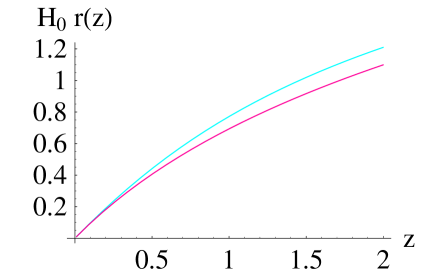
In Figure 1 the dimensionless coordinate distance $H_{0}r(z)$ as a function of redshift $z$ is shown. Our quantum model is drawn as a lower red line. It describes the expansion of the universe as a whole at a steady rate (with vanishing deceleration parameter $q(z)\equiv-\ddot{a}a/\dot{a}^{2}$). The upper blue line corresponds to the model with dark energy in the form of cosmological constant whose contribution to the total energy density is equal to 70 %. The latter phenomenological model predicts an accelerated expansion of the present-day universe with the following deceleration parameter: $q_{0}=-0.55$.

Figure 1: Dimensionless coordinate distance $H_{0}\,r(z)$ vs. $z$ in quantum model (lower red line) and in $\Lambda$CDM-model with $\Omega_{X}=0.7$ and present-day deceleration parameter $q_{0}=-0.55$ (upper blue line).

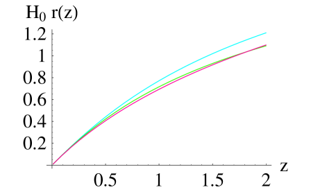
In Figure 2 extra middle green line is added. It corresponds to the model with cosmological constant whose contribution to the total energy density is equal to 56 % . The present-day deceleration parameter for such a model is the following: $q_{0}=-0.34$. The rest as in Figure 1. The red line which represents our quantum model practically coincides with the green line of the model with smaller acceleration. But it is worth to note that these two models describe the different physics.

Figure 2: Dimensionless coordinate distance $H_{0}\,r(z)$ vs. $z$ in quantum model (lower red line) and in $\Lambda$CDM-models with $\Omega_{X}=0.56$ and $q_{0}=-0.34$ (middle green line) and $\Omega_{X}=0.7$ and $q_{0}=-0.55$ (upper blue line).

In Figure 3 the three above mentioned models are compared with the observational data. The type Ia supernovae are shown as solid circles. From more then 170 objects of the survey we have drawn only a few dozens of typical supernovae which allow to follow the general tendency.

Figure 3: Dimensionless coordinate distances $H_{0}\,r(z)$ to supernovae at redshift $z$. The observed SNe Ia [Riess et al. 2004], [Daly & Djorgovski 2004] are shown as solid circles. The rest as in Fig. 2.

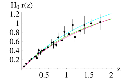
We may conclude that our quantum model is entirely consistent with the data of observations. This conclusion agrees with the result of data processing by [Daly & Djorgovski 2004] who demonstrate that the model with lower value of the contribution from dark energy in the form of cosmological constant (the green line in Figures 2 and 3) may be preferred.

4.3 Quantum fluctuations of scale factor

Deviations of the coordinate distances $H_{0}\,r(z)$ from the logarithmic law (34) towards both larger and smaller distances for some supernovae can be explained by the local manifestations of quantum fluctuations of scale factor about its average value $\langle a\rangle$. Such fluctuations arose in the Planck epoch ($t\sim 1$) due to finite widths of quasistationary states. They can cause the formation of nonhomogeneities of matter density which have grown with time into the observed large-scale structures in the form superclusters and clusters of galaxies, galaxies themselves etc. [Kuzmichev & Kuzmichev 2002].

Let us consider the influence of mentioned fluctuations on visible positions of supernovae. The position of quasistationary state can be determined only approximately, $|\delta\epsilon_{n}|\sim\Gamma_{n}$, and the scale factor of the universe in the $n$-th state can be found only with an uncertainty $\delta a\gtrless 0$,

$$\epsilon_{n}\rightarrow\epsilon_{n}+\delta\epsilon_{n}\qquad\Rightarrow\qquad\langle a\rangle\rightarrow\langle a\rangle+\delta a.$$

If one assumes that just the fluctuations of the scale factor $\delta a$ cause deviations of positions of sources at high redshift from the logarithmic law (34), then the coordinate distances will be given by the following expression

$$H_{0}\,r(z)=\ln\left[\left(1+\frac{\delta a}{\langle a\rangle}\right)^{-1}(1+z)\right].$$ (35)

The possible values of coordinate distances in quantum model which takes into account fluctuations are shown as an area between two orange lines in Figure 4. Practically all supernovae fall within the shown limits.

Figure 4: Dimensionless coordinate distances $H_{0}\,r(z)$ to supernovae at redshift $z$. An area between two orange lines corresponds to possible values of coordinate distances in quantum model with fluctuations.

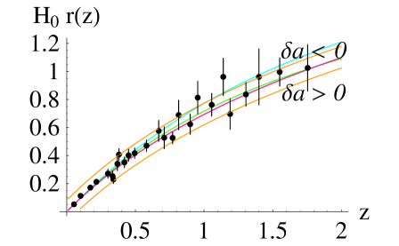
Thus the observed faintness of the SNe Ia can in principle be explained by the logarithmic-law dependence of coordinate distance on redshift in generalized form (35) which takes into account the fluctuations of scale factor about its average value. These fluctuations can arise in the early universe and grow with time into observed deviations of the coordinate distances of separate supernovae at the high redshift. They produce accelerating or decelerating expansions of space subdomains containing such sources whereas the universe as a whole expands at a steady rate.

The same analysis one can make for radio galaxies as well.

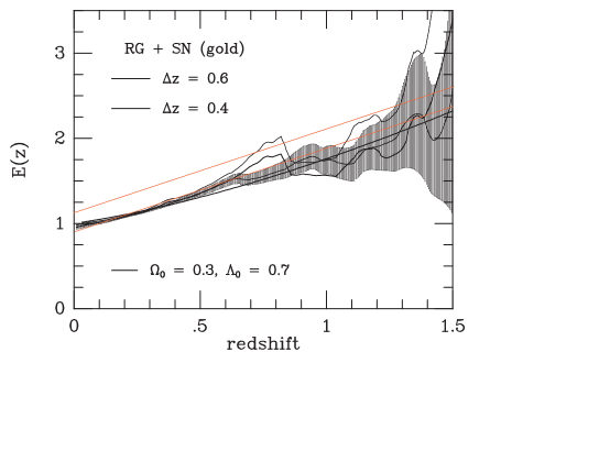
One can come to a conclusion that the universe as a whole expands at a steady rate analyzing the information about the expansion rate extracted directly from the data on coordinate distances to supernovae and radio galaxies.

In Figure 5 the derived values of the dimensionless expansion rate $E(z)\equiv(\dot{a}/a)H_{0}^{-1}$ obtained by [Daly & Djorgovski 2004] are shown. The inaccuracy of measurements and uncertainties in data processing do not allow to take this plot as a final outcome, but only look at the global trends. These trends are supported by the results of our calculations drawn in Figure 5 as an area between the red lines.

Figure 5: The dimensionless expansion rate vs. redshift [Daly & Djorgovski 2004], $E(0)=0.97\pm 0.03$. An area between two red lines corresponds to possible values of dimensionless expansion rate in quantum model with fluctuations.

The proposed approach to the explanation of observed dimming of some SNe Ia may provoke objections in connection with the problem of large-scale structure formation in the universe, since the energy density $\langle\rho_{tot}\rangle$ in the form (29) cannot ensure an existence of a growing mode of the density contrast $\delta\langle\rho_{tot}\rangle/\langle\rho_{tot}\rangle$ (see e.g. [Weinberg 1972]). As we have already mentioned above the density $\langle\rho_{tot}\rangle$ (29) describes only homogenized properties of the universe as a whole. It cannot be used in calculations of fluctuations of energy density about the mean value $\langle\rho_{tot}\rangle$. Under the study of large-scale structure formation one should proceed from the more general expression for the energy density (28). Defining concretely the contents of matter/energy $M$, as for instance in the model of creation of matter and energy proposed in [Kuzmichev & Kuzmichev 2004b], one can make calculations of density contrast as a function of redshift. The ways to solve the problem of large-scale structure formation in the quantum model are roughly outlined in [Kuzmichev & Kuzmichev 2002].

4.4 Dark matter and dark energy prediction

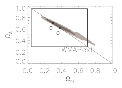
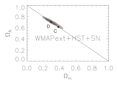
The quantum model allows to calculate the percentage of the mass-energy constituents in the total energy density. For a flat universe it predicts 29 % for the matter density and 71 % for the dark energy contribution (for details see [Kuzmichev & Kuzmichev 2004b]).

In Figures 6 and 7 the theoretical values of matter density and dark energy density in comparison with observational data summarized by
[Spergel et al. 2003] are shown.

There is a good agreement between combined observational data and the theoretical prediction.

Acknowledgements. I would like to thank the organizers (Bogolyubov Institute for Theoretical Physics, National Academy of Sciences of Ukraine, Ukrainian Physical Society, University of California), especially Professor L. Jenkovszky, for the invitation to participate in the workshop.

Figure 6: The plane $\Omega_{\Lambda}\equiv\Omega_{X}/\Omega_{tot}$ vs. $\Omega_{m}\equiv\Omega_{M}/\Omega_{tot}$. Constraints on the density components determined using WMAP + other CMB experiments [Spergel et al. 2003]. The acceptable values of $\Omega_{\Lambda}$ and $\Omega_{m}$ lie on the diagonal of rectangle. The central value of the region is shown as a solid box C. The point D corresponds to the case $Q\simeq 10$ GeV, $Q$ is the energy released in decay of elementary quantum excitation of the vibrations of the scalar field.

Figure 7: Constraints on the density of matter $\Omega_{m}$ and dark energy $\Omega_{\Lambda}$ determined using WMAPext + HST key project data + supernova data [Spergel et al. 2003]. The rest as in Fig. 6.

References

- [Ambrus & Hájíček 2001] Ambrus, M. & Hájíček, P. 2001, Phys. Rev. D63, 104017; gr-qc/0012002.
- [de Bernardis et al. 2000] de Bernardis, P. et al. 2000, Nature, 404, 955.
- [Cole et al. 2001] Cole S. M. et al. 2001, MNRAS, 326, 255.
- [Daly & Djorgovski 2004] Daly, R. A. & Djorgovski, S. G. 2004, to appear in Astrophys. J., 612; astro-ph/0403664.
- [Fock 1976] Fock, V. A. 1976, Nachala kvantovoi mekhaniki (Foundation of Quantum Mechanics), Nauka, Moscow.
- [Fukugita & Peebles 2004] Fukugita, M. & Peebles, P. J. E. 2004, astro-ph/0406095.
- [Isham 1995] Isham, C. J. 1995, lecture given at the GR14 conference, Florence, August 1995; gr-qc/9510063.
- [Kiefer 1999] Kiefer, K. 1999, in Lecture Notes in Physics 541 “Towards Quantum Gravity”, ed. J. Kowalski-Glikman, (Springer-Verlag, 2000), p. 158; gr-qc/9906100.
- [Krauss 2003] Krauss, L. M. 2003, astro-ph/0301012.
- [Kuchař & Torre 1991] Kuchař, K. V. & Torre, C. G. 1991, Phys. Rev. D43, 419.
- [Kuzmichev 1998] Kuzmichev, V. V. 1998, Ukr. J. Phys., 43, 896.
- [Kuzmichev 1999] Kuzmichev, V. V. 1999, Phys. At. Nucl., 62, 708; gr-qc/0002029.
- [Kuzmichev & Kuzmichev 2002] Kuzmichev, V. E. & Kuzmichev, V. V. 2002, Eur. Phys. J. C, 23, 337; astro-ph/0111438.
- [Kuzmichev & Kuzmichev 2004a] Kuzmichev, V. E. & Kuzmichev, V. V. 2004a, to appear in “Progress in General Relativity and Quantum Cosmology Research” (Nova Science Publishers, 2004); astro-ph/0405454.
- [Kuzmichev & Kuzmichev 2004b] Kuzmichev, V. E. & Kuzmichev, V. V. 2004b, to appear in “Progress in Dark Matter Research” (Nova Science Publishers, 2004); astro-ph/0405455.
- [Netterfield et al. 2002] Netterfield, C. B. et al. 2002, Astrophys. J., 571, 604; astro-ph/0104460.
- [Peebles & Ratra 2003] Peebles, P. J. E. & Ratra, B. 2003, Rev. Mod. Phys., 75, 599; astro-ph/0207347.
- [Pryke et al. 2002] Pryke, C. et al. 2002, Astrophys. J., 568, 46; astro-ph/0104490.
- [Riess et al. 2004] Riess, A. G. et al. 2004, astro-ph/0402512.
- [Salucci & Persic 1999] Salucci, P. & Persic, M. 1999, MNRAS, 309, 923.
- [Sievers et al. 2003] Sievers, J. L. et al. 2003, Astrophys. J., 591, 599; astro-ph/0205387.
- [Spergel et al. 2003] Spergel, D. N. et al. 2003, Astrophys. J. Suppl., 148, 175; astro-ph/0302209.
- [Tonry et al. 2003] Tonry, J. L. et al. 2003, Astrophys. J., 594, 1; astro-ph/0305008.
- [Weinberg 1972] Weinberg, S. 1972, Gravitation and Cosmology, Wiley.