Abstract

Young massive stars produce Far-UV photons which dissociate the molecular gas on the surfaces of their parent molecular clouds. Of the many dissociation products which result from this “back-reaction”, atomic hydrogen H i is one of the easiest to observe through its radio 21-cm hyperfine line emission. In this paper I first review the physics of this process and describe a simplified model which has been developed to permit an approximate computation of the column density of photodissociated H i which appears on the surfaces of molecular clouds. I then review several features of the H i morphology of galaxies on a variety of length scales and describe how photodissociation might account for some of these observations. Finally, I discuss several consequences which follow if this view of the origin of HI in galaxies continues to be successful.

[Photodissociation and the Morphology of H i in Galaxies] Photodissociation and the
Morphology of H i in Galaxies

1 Introduction

I want to begin this talk with a brief discussion of some aspects of the astrophysics of photodissociation regions (PDRs) in order to make it clear that the production of H i from H₂ in the ISM is quite inevitable, and that the cycling of H i $\leftrightarrow$ H₂ is likely to be both continuous and ubiquitous in galaxies. I will then move on to a brief description of some of the features of the H i morphology of galaxies which appear to be amenable to an explanation in terms of PDR astrophysics.

The material presented here is a review of results and views published by myself and by others in previous journal and conference papers. New in this paper are some preliminary results on the effects of radial gradients in the metallicity of the ISM on the overall H i distribution in galaxies in the context of the photodissociation picture described here.

2 H i from photodissociation of H₂ in the ISM

The physics and astronomy of the photodissociation $\leftrightarrow$ reformation process for molecules in the ISM is a subject of active research, and an excellent review of the field was published a few years ago by [Hollenbach & Tielens(1999)]. The results have been successfully applied to star-forming regions in the Galaxy on length scales of typically 0.1 - 1 pc. The first indication that photodissociation may be operating to affect the large-scale morphology (100-1000 pc) of the H i in galaxies was found in M83 by [Allen, Atherton & Tilanus(1986)], who noticed a clear spatial separation between a particularly well-defined dust lane several kiloparsec long and the associated ridge of H i and H ii in the southern spiral M 83. Appropriately for this conference, M 83 is a barred spiral galaxy, and the strong stellar density wave which is apparently driven by the bar has produced large streaming velocities in the gas across the arms, leading to a measureable separation of various phases of the ISM.

Dissociation of H₂ by far-UV photons

It requires a photon of energy $\geq 14.67$ eV to lift an H₂ molecule directly from its ground state to the electronic continuum. Such photons will be rare in the ISM since they are strongly absorbed in ionizing H i to H ii. For this reason it was initially thought ([Spitzer(1948)]) that H₂ would be very long-lived in the ISM. However, closer examination of the electronic and vibrational energy-level diagram for H₂ revealed another dissociation channel. In this “fluorescence” process, less energetic photons can raise the H₂ molecule to an excited electronic state. When the molecule decays to the ground electronic state, it can end up in a variety of excited vibrational states. However, vibrational levels above 14 are so energetic that they break the chemical bond holding the H₂ molecule together, and two H i atoms are produced. A quantitative description of this process was first given by [Stecher & Williams(1967)]. It starts when H₂ molecules absorb photons primarily at wavelengths of $\lambda\approx 110.8$ and $\approx 100.8$ nm through transitions to the to the electronically-excited Lyman ($X^{1}\Sigma_{g}^{+}\rightarrow B^{1}\Sigma_{u}^{+}$) and Werner ($X^{1}\Sigma_{g}^{+}\rightarrow C^{1}\Pi_{u}^{+}$) bands. In the subsequent decay to various vibrationally-excited levels of the ground electronic state, $\sim 10-15$% of the H₂ molecules will dissociate into two H i atoms. Considering that even higher electronic states exist in H₂, it is clear that the FUV spectrum over the whole range from 91.2–110.8 nm (13.6–11.2 eV) contributes to the dissociation. In high-UV-flux environments ($G_{0}$ $\gtrsim 10^{4}$, [Shull(1978)]), photons with wavelengths as long as $\approx 185$ nm ($\approx 6.6$ eV) can continue to create H i by dissociating “pumped” H₂ ($X^{1}\Sigma_{g}^{+},2<v\leq 14$) via additional Lyman- and Werner-band transitions. Verification that this process actually occurs in the ISM was obtained when the predicted UV fluorescence spectrum was first observed by [Witt et al.(1989)] in the Galactic nebula IC 63.

Using the notation of [Sternberg(1988)], the rate at which H₂ is dissociated by this process in the ISM per unit volume can be written as:

$$R_{diss}=D\chi\times e^{-\tau_{gr,1000}}\times f_{s}(N_{2})\times n_{2},$$ (1)

in units of H₂ molecules dissociated ${\rm cm^{-3}}$ sec^-1, where $n_{2}=n$(H₂), and

$D$ = the unattenuated H₂ photodissociation rate in the average ISRF, $\chi$ = the incident UV intensity scaling factor, $\sigma$ = the effective grain absorption cross section per H nucleus in the FUV continuum, $\tau_{gr,1000}$ = $\sigma(N_{1}+2N_{2})$ is the dust grain opacity at $\lambda\sim 100$ nm, and $n$ = $n_{1}+2n_{2}$ the volume density of H nuclei.

Since $D=5.43\times 10^{-11}$ s^-1 (according to the simplified 3-level model, [Sternberg(1988)]) the time scale for this process on the surface of a typical GMC ($n_{2}\sim 50$ molecules ${\rm cm^{-3}}$) illuminated by the ISRF is $\tau_{diss}=(Dn_{2})^{-1}\approx 10$ yr! Note that each dissociation produces two H i atoms on the cloud surface, and the appearance of a layer of H i when a FUV radiation field is “switched on” (e.g. from the birth of a new O–B star) is instantaneous compared to most other time scales in the ISM.

Formation of H₂ on dust grains

Formation of H₂ occurs in the ISM most efficiently on dust grains (cf. e.g. [Hollenbach & Tielens(1999)] and references cited there). The model for the formation rate depends on several parameters (some of which are not accurately known), as well as on the nature of the dust grains (which may vary from place to place in a galaxy). The usual parametrization is:

$$R_{form}=\gamma_{2}\times n\times n_{1}$$ (2)

in units of H₂ molecules ${\rm cm^{-3}}$ sec^-1, and $n=n_{1}+2n_{2}$. The rate coefficient for unit density, solar metallicity, and 100K kinetic temperature (roughly the ISM in the solar neighborhood) is $\sim$ $1-3\times 10^{-17}$ cm³ sec^-1. This equation is strongly dependent upon the dust–to–gas ratio ($\delta=A_{V}/N_{H}$) and weakly dependent upon the gas temperature ($T$), since

$$\gamma_{2}=3.0\times 10^{-18}(\delta/\delta_{0})T^{1/2}y_{F}(T)\ {\rm cm^{3}\ s^{-1}},$$

where $\delta_{0}$ refers to the value of $\delta$ in the solar neighborhood, and $y_{F}(T)$ represents the efficiency of H₂ formation. The product $T^{1/2}y_{F}(T)$ is thought to be constant to within a factor of 2 ([Hollenbach et al.(1971)]).

The time scale for this process is $\tau_{form}=(2n\gamma_{2})^{-1}\approx$ $5\times 10^{8}$/$n$ yr, and this will be the rate-determining time scale in an equilibrium situation where photodissociation is balanced by reformation on dust grains.

Equilibrium

In recent years, much effort has gone into calculating the level populations of the ro-vibrational lines of the ground state of H₂, and the intensities of the associated quadrupole line emission. These lines can be observed with space missions (e.g. SWAS, ISO) in PDRs in the Galaxy and in the nuclear regions of other galaxies. The H i column density in a PDR is calculated with the same physics used to determine the excitation of the H₂ near-infrared fluorescence lines. While the computations for those lines are rather complicated, the determination of H i column can be obtained from a simplified version of the model. Furthermore the 21-cm line emission from H i is almost always optically thin, so the observations usually yield the H i column directly for comparison with the model. The formation and destruction rates described above are set equal, and the equation solved, in the present case for the H i column density. A logarithmic form for the analytic solution to this equation was first given by [Sternberg(1988)]; see also Appendix A of this paper for a brief derivation. Other relevant references are given in [Allen et al.(2004)]. The model is a simple semi-infinite slab geometry in statistical equilibrium with FUV radiation incident on one side. The solution gives the steady state H i column density along a line of sight perpendicular to the face of the slab as a function of $\chi$, the incident UV intensity scaling factor, and the total volume density $n$ of H nuclei. Sternberg’s result is:

$$N(\mbox{H\,{\sc i}})={1\over\sigma}\times\ln{\left[{{D\mathcal{G}}\over{\gamma_{2}n}}\chi+1\right]},$$ (3)

$D$	=	the unattenuated H2 photodissociation rate in the average ISRF,
$\gamma_{2}$	=	the H2 formation rate coefficient on grain surfaces,
$\sigma$	=	the effective grain absorption cross section
		per H nucleus in the FUV continuum,
$\chi$	=	the incident UV intensity scaling factor,
$N(\mbox{H\,{\sc i}})$	=	the H i column density,
$n$	=	the volume density of H nuclei.

Equation 3 has been developed using a simplified three-level model for the excitation of the H₂ molecule and is applicable for low-density ($n\lesssim 10^{4}$ ${\rm cm^{-3}}$), cold (T $\lesssim 500$ K), isothermal, and static conditions, and neglects contributions to $N(\mbox{H\,{\sc i}})$ from ion chemistry and direct dissociation by cosmic rays. The quantity $\mathcal{G}$ here (not to be confused with $G_{0}$ to be defined momentarily) is a dimensionless function of the effective grain absorption cross section $\sigma$, the absorption self–shielding function $f_{s}(N_{2})$, and the column density of molecular hydrogen $N_{2}$:

$$\mathcal{G}=\int_{0}^{N_{2}}\sigma f_{s}e^{-2\sigma N_{2}^{\prime}}{\rm d}N_{2}^{\prime}.$$

The function $\mathcal{G}$ becomes a constant for large values of $N_{2}$ due to self–shielding ([Sternberg(1988)]). Using the parameter values in this equation adopted by [Madden et al.(1993)], we have:

$$N(\mbox{H\,{\sc i}})=\mbox{$5\times 10^{20}$}\times\ln[1+(90\chi/n)]$$

where $n$ is in ${\rm cm^{-3}}$. This is a steady state model, with H₂ continually forming from H i on dust grain surfaces, and H i continually forming from H₂ by photodissociation.

Equation 3 is strongly dependent upon the dust–to–gas ratio ($\delta=A_{V}/N_{H}$) and weakly dependent upon the gas temperature ($T$), since

$$\sigma = 1.883\times 10^{-21}(\delta/\delta_{0})\ {\rm cm}^{-2},$$

$$\gamma_{2} = 3.0\times 10^{-18}(\delta/\delta_{0})T^{1/2}y_{F}(T)\ {\rm cm^{3}\ s^{-1}},$$

$$\mathcal{G} = (\sigma/\sigma_{0})^{1/2}\mathcal{G_{O}},$$

where $\delta_{0}$, $\sigma_{0}$, and $\mathcal{G_{O}}$ refer to values in the solar neighborhood, and $y_{F}(T)$ represents the efficiency of H₂ formation. The product $T^{1/2}y_{F}(T)$ is thought to be constant to within a factor of 2 ([Hollenbach et al.(1971)]).

Equation 3 also contains a dependence on the level of obscuration in the immediate vicinity of the FUV source. While the variable $\chi$ represents the intrinsic FUV flux associated with the star-forming region, we generally observe an attenuated FUV flux. Assuming any extinction associated with the star-forming region is in the form of an overlying screen of optical depth $\tau(FUV)$, $\chi({\rm observed})=\chi e^{-\tau(FUV)}$. However, an accurate correction for this effect may be difficult, Since the ISM in the immediate vicinity of the FUV source will have been disturbed by stellar winds and any prior supernovae.

Assuming solar neighborhood values of $\sigma_{0}=1.883\times 10^{-21}$ cm², $D=5.43\times 10^{-11}$ s^-1, $\gamma_{20}=3\times 10^{-17}$ cm³ s^-1, and $\mathcal{G_{O}}\approx 5\times 10^{-5}$ ([Sternberg(1988)]), and neglecting the weak temperature dependence of $\gamma_{2}$, equation 3 becomes:

$$N(\mbox{H\,{\sc i}})={{5\times 10^{20}}\over{(\delta/\delta_{0})}}\ln{\left[{{90\chi}\over{n}}{{\left({{\delta}\over{\delta_{0}}}\right)}^{-1/2}}+1\right]},$$ (4)

where $\chi=\chi({\rm observed})e^{\tau(FUV)}$.

Figure 1: The Relationship between $N(\mbox{H\,{\sc i}})$ and $\chi$. The observed and predicted values of $N(\mbox{H\,{\sc i}})$ are shown as a function of $\chi$. The modeled behavior of $N(\mbox{H\,{\sc i}})$ assumes values of $\delta/\delta_{0}=0.2$ and $\tau(FUV)=0$, appropriate for the outer regions of M101. The observations are clearly consistent with the physics underlying the photodissociation picture.

The behavior of $N(\mbox{H\,{\sc i}})$ as a function of $\chi$ is displayed for $\delta/\delta_{0}=0.2$, $\tau(FUV)=0$ and $n=30$, $n=300$, and $n=3000$ in Figure 1. These values of $\delta/\delta_{0}$ and $\tau(FUV)$ are appropriate for the outer regions of M101, as discussed in [Smith et al.(2000)]. Values of $N(\mbox{H\,{\sc i}})\gtrsim 10^{22}$ cm^-2 are not likely to be observed as the atomic gas probably becomes optically thick at this point:

$$N(\mbox{H\,{\sc i}}) = 1.82\times 10^{18}\int_{-\infty}^{\infty}T_{s}\tau(v)dv$$

$$\rightarrow 1.82\times 10^{18}T_{s}\tau\Delta v$$

$$\approx 10^{22}{\rm cm}^{-2},$$

for spin temperatures of $T_{s}\approx 100$K and profile FWHMs of $\Delta v\approx 20$ km s^-1 typical of M101 ([Braun(1997)]), and for optical depths of $\tau\approx 2.5$, corresponding to a ratio between the brightness and kinetic temperatures of $T_{B}/T_{K}\approx 0.9$. This value is appropriate for the highest-brightness regions of M101, as indicated in Figure 8a of [Braun(1997)]. Figure 1 also shows the measurements for each of the 35 candidate PDRs in M101 as analysed by [Smith et al.(2000)]. The data indicate that the properties of observed regions in M101 are consistent with photodissociation of an underlying molecular gas of moderate volume density.

[Allen et al.(2004)] have recently re-examined equation 4 and compared it with the full numerical treatment used in the “standard” Ames model summarized in [Kaufman et al.(1999)]. A conversion of the FUV flux $\chi$ used by [Sternberg(1988)] to the quantity $G_{0}$ used by [Kaufman et al.(1999)] is first required; this is because [Sternberg(1988)] and [Kaufman et al.(1999)] use different normalisations for the FUV flux (see Appendix B in [Allen et al.(2004)]). When distributed sources illuminate an FUV-opaque PDR over $2\pi$ sr, the conversion is $\chi=G_{0}/0.85$ (see Footnote 7 in [Hollenbach & Tielens(1999)]), resulting in $90\chi/n=106G_{0}/n$. With this change, [Allen et al.(2004)] fitted the analytic expression for $N(\mbox{H\,{\sc i}})$ above to the model computations in the range in which cosmic ray dissociation is not a major contributor, roughly for $G_{0}$ $\gtrsim 1$, $n\gtrsim 10$ ${\rm cm^{-3}}$. The result is that no consistent improvement is obtained by using any value for the coefficient of $G_{0}$ other than the value 106 deduced above, although a modest improvement is obtained by using a slightly larger value for the leading coefficient in the equation, $7.8\times 10^{20}$, corresponding to a value of $1.3\times 10^{-21}$ cm² for the effective grain absorption cross section. With these small adjustments, the final best-fit equation is:

$$N(\mbox{H\,{\sc i}})={{7.8\times 10^{20}}\over{(\delta/\delta_{0})}}\ln{\left[{{106G_{0}}\over{n}}{{\left({{\delta}\over{\delta_{0}}}\right)}^{-1/2}}+1\right]}{\rm~{}cm}^{-2},$$ (5)

where $n=n(HI)+2n(H_{2})$ and $G_{0}$ and $\delta_{0}$ are the (normalized) FUV flux and dust/gas ratio in the ISM of the solar neighborhood.

Figure 2: Contours of constant H i column density $N(\mbox{H\,{\sc i}})$ in units of $10^{21}$ ${\rm cm^{-2}}$ in the PDR as a function of the density $n$ and incident FUV flux $G_{0}$ for the standard model parameters in [Kaufman et al.(1999)] (dotted lines), and for the analytic approximation of eq. 5 (solid lines). The labeled contour values are for the numerical model; the contours for the analytic model start from $10^{-3}$ (lower right corner) and increase to $10^{-2}$, $10^{-1}$, 1, 3, 5, 7, and end at 10 (upper left corner).

In Figure 2 we show values from equation 5 plotted as solid lines together with dotted contour lines from the “standard” numerical model for $\delta=\delta_{0}$. The agreement is generally good over much of the $n$–$G_{0}$ parameter space of interest here; differences occur mainly in the top left corner of the diagram, and at low values of FUV flux. In the top left corner the analytic formula under-predicts the amount of H i column density computed from the standard model by about 30% owing to H i production by ion chemistry reactions such as $H_{2}^{+}+H_{2}\rightarrow H_{3}^{+}+H$, $HCO^{+}+e^{-}\rightarrow CO+H$, and $PAH^{-}+H^{+}\rightarrow PAH+H$ (where PAH is a polycyclic aromatic hydrocarbon), which are important at high $G_{0}$ and low $n$. At values of $G_{0}$ $\lesssim 1$ the contours of $N(\mbox{H\,{\sc i}})$ for the numerical model become vertical; this is because the standard model includes a low level of cosmic ray ionization which contributes a small amount of H i by dissociation of H₂ even for $G_{0}$ = 0.

It should be noted that both the analytic and the numerical forms depend on several rather crude parameters used to describe the properties of the gas – dust mixture in the ISM (dust cross section, H i sticking coefficients, etc.), and that not all proponents of PDR models use the same values for these parameters. A coordinated effort is presently taking place among the modellers, first to see if different PDR codes can produce the same results when using the same numerical values for parameters (no, they can differ, and sometimes by a lot!), and second, to try to reach some agreement on an acceptable set of values for these parameters.

There are several noteworthy aspects of this equation:

• $N(\mbox{H\,{\sc i}})$ depends only on the ratio of $G_{0}/n$. Low FUV flux, low density environments in galaxies can produce the same column of H i found in high flux, high density environments. The difference will be in the thickness of the H i layer; much thicker layers of H i are associated with the low flux, low density environments;

• at a given $n$, $N(\mbox{H\,{\sc i}})$ increases first linearly with $G_{0}$, but then “saturates” and increases only logarithmically after that;

• at a given $G_{0}$, $N(\mbox{H\,{\sc i}})$ decreases logarithmically with increasing $n$, and;

• the H i column decreases as the dust/gas ratio increases.

3 Time scales

As discussed in the previous section, the relevant time scale for the production of H i on the surfaces of molecular clouds is the formation time for H₂ on dust grains. The full expression including the dust/gas dependence is:

$$\tau_{2} = (2n\gamma_{2})^{-1}$$ (6)

$$= \frac{5\times 10^{8}}{(n_{1}+2n_{2})\times(\delta/\delta_{0})}\ \mbox{\rm yrs.}$$

Table 1 gives typical values for $\tau_{2}$ in several different environments in the ISM, and Table 2 lists a number of time scales set by other processes in galaxy disks.

Table 1: H i production time scales in typical ISM environments.

Environment	$n$	$\delta/\delta_{0}$	$\tau$ (years)
Solar metallicity GMC	100	1	$\sim 3\times 10^{6}$
Intercloud gas	10	1	$\sim 3\times 10^{7}$
Outer galaxy GMC	100	0.1	$\sim 3\times 10^{7}$

Table 2: Other time scales in galaxies.

Situation	Time scale (years)
GMC crossing time $R/\Delta V$	$\sim 7\times 10^{6}$
Spiral arm crossing time	$\sim 5\times 10^{7}$
B3 star lifetime for FUV production	$\sim 5\times 10^{7}$
Galaxy rotation time	$\sim 5\times 10^{8}$
Hubble time	$\sim 10^{10}$

It is clear that the time scale for H i production by photodissociation of H₂ is short enough to be relevant. For instance, H i is produced in the same time scales as that of molecular cloud formation ([Pringle, Allen & Lubow(2001)]) and of the star formation in those molecular clouds ([Elmegreen(2000)]), and in a tenth of the lifetime of a typical B star for FUV photon producation. This must be the reason why we see H i in regions where young stars form, and why H i appears in “rims” around clusters of B stars in spiral arms. H i also appears in a time short compared to the time it takes for a GMC to cross a spiral arm, and the H i will correspondingly disappear as the FUV production ceases further down stream and the gas reverts to a predominantly molecular form. Even in the far outer parts of galaxies we see that the H i time scale is still only about 10% of the rotation time of the galaxy, so for undisturbed galaxies we can expect an equilibrium to obtain between H i and H₂ even in these sparse environments.

4 Major features in the H i morphology of galaxies

Our picture of the major features of the H i morphology in disk galaxies has closely followed the steady improvements in angular resolution of centimeter-wave radio telescopes, first with filled apertures (Dwingeloo, NRAO 300’, Parkes, Arecibo, GBT…), and later with synthesis imaging instruments (Westerbork, VLA, ATNF…).

Radial distribution of H i surface brightness

Figure 3: Radial distribution of H i surface brightness for the nearby giant Sc galaxy NGC5457 = M 101 obtained by averaging the H i data in annular elliptical rings. From [Braun(1997)], adjusted to an assumed distance of 5.4 Mpc. $R_{25}$ for this galaxy is $13.5^{\prime}\approx 21$ kpc.

A typical averaged H i radial surface brightness profile of a nearby giant Sc galaxy is shown in Figure 3. The main features to notice are:

• the central depression;

• the “flat top”, typically at a level of $5-10\times 10^{20}$ ${\rm cm^{-2}}$, and;

• the long “tail” to faint levels in the distant outer parts.

What parts of this plot can be explained by the photodissociation picture descibed in the previous section? An explanation for the “flat top” was actually suggested in terms of the photodissociation picture nearly 20 years ago by [Shaya & Federman(1987)], but I fear that paper has been widely ignored by most workers in the field of extragalactic H i and H₂. A good look at equation 5 makes it clear: owing to the logarithmic dependence of N(H i) on the ratio $G_{0}$/$n$ and the fact that the largest concentrations of young stars also go along with regions of highest gas density, we ought not to expect values of H i column density much in excess of a few times the coefficient in front of the log. So even in the most active starbursting regions of galaxies, we are not likely to observe values of the H i column density much in excess of $\sim$ $few\times 10^{21}$ ${\rm cm^{-2}}$. As to the decline in the outer regions, this is likely to be a combined effect of a declining ambient FUV flux and a declining area filling factor, since [Smith et al.(2000)] have shown that the total gas density $n$ on the surfaces of GMCs located in the neighborhood of massive young stars does not appear to change much with radius.

Finally, the depression in the inner parts can be explained as a consequence of the general increase in the metallicity of the ISM in the inner parts of galaxy disks. In Figure 4 my student colleague Ben Waghorn has fitted equation 5 to the combined radial data on the FUV distribution and the metallicity gradient in M 101. The free parameters are the H i area filling factor (taken here to be 0.3 everywhere), and the GMC gas volume density $n$ (fits shown for 100, 200, and 300 ${\rm cm^{-3}}$). We see that, in spite of the strong increase in FUV flux $G_{0}$ in the inner parts of the galaxy, the rapid rise of the dust/gas ratio (assumed proportional to the O/H ratio) actually results in a decrease in N(H i), as observed, and the quantitative fit is also reasonable. I note here that this result has already been described by [Smith et al.(2000)] for a small subset of young star clusters in M 101 accounting for only a few percent of the total H i content of the galaxy; what we are now seeing is that the same explanation appears viable for all the H i in the galaxy. We have examined nearly a dozen nearby spirals in this way, and find reasonable agreement for about half of them. The other half show an indication that there is more H i present than FUV-related photodissociation can explain. Interestingly, these galaxies nearly all have bright nonthermal radio continuum disks, suggesting that there is a component of the H i being maintained from dissociation by cosmic rays penetrating throughout the GMCs. This work is ongoing.

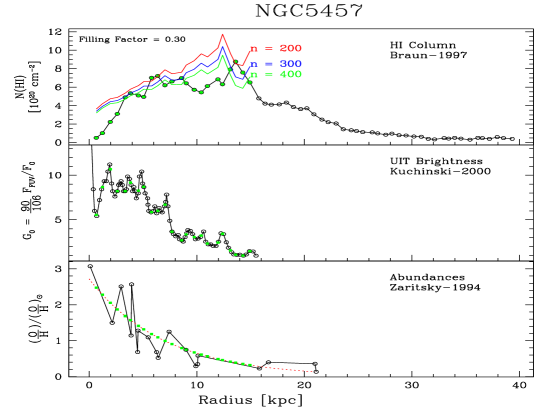
Figure 4: H i column density (top), FUV brightness (middle), and O/H ratio (lower) as a function of radius for M 101. Equation 5 has been used to produce the fits shown in the top panel for an area filling factor of 0.3 and $n=100,200,\&\ 300$ ${\rm cm^{-3}}$. From work in progress by Allen, Waghorn, & Heiner.

Spiral structure

In the Introduction to this paper I pointed out that it was thanks to a strong density wave in the southern barred spiral M 83 that the importance of photodissociation in affecting the morphology of galaxies on the large scale was first unmasked. Other studies have followed on M83 and on other galaxies (M 51, M 100; see [Smith et al.(2000)] for references) and have generally agreed that the initial interpretation in terms of photodissociation remains the most viable option. The separation in the case of M 83 is about 250 pc, and arises because of the difference between the spiral pattern speed and the rotation speed of the gas, coupled with the time for collapse of GMCs and the time that a massive young star lives on the main sequence.

The clear existence of spiral features in the H i distribution of a galaxy external to our own was perhaps first convincingly demonstrated for M 101 by [Allen, Goss, & Van Woerden(1973)]. Although this galaxy apparently does not have a very strong density wave, the H i is arranged in thin spiral segments which appear in the inner disk and can be traced over a large part of the main body of the galaxy right out to beyond $R_{25}$. Figure 5 shows the H i image (grey, kindly provided in digital form by R. Braun) with the FUV contours superposed ([Smith et al.(2000)]). The correspondence is excellent, at least as far out in the disk as the UIT data extend. We expect to see the FUV image and spiral features grow further when the GALEX data become available later this year, and we can confidently predict that the close correspondence with the H i will continue.

Figure 5: The distribution of atomic hydrogen as seen at a resolution of $6^{\prime\prime}\approx 200$ pc in M 101 ([Braun(1995)]). Thin, prominent spiral arms wind outwards to beyond the optical disk at $R_{25}\approx 13.5^{\prime}$, with the outer H i arms generally traceable back to arms which start in the main body of the disk. Contours of the Far-UV emission recorded by UIT are superposed. From the PDR analysis by [Smith et al.(2000)].

H i arcs and blisters

The first study to successfully identify the characteristic PDR “arc” or “blanket” morphology of H i in close association with far-UV sources in a nearby galaxy was carried out on M81 by [Allen et al.(1997)]. The problem is, of course, to obtain sufficient linear resolution ($\sim 100$ pc) in the H i observations to permit one to identify the morphology of the PDR structures. An important point to note is that the best “correlation” is between the H i and the far-UV, and not between the H i and the H$\alpha$.

A study similar to that done on M81 but with more quantitative results has been carried out on M101 by [Smith et al.(2000)], who used VLA-H i and UIT far-UV data to identify and measure PDRs over the whole extent of the M101 disk. From these observations they derived the volume density of the H₂ in the adjacent GMCs in the context of the PDR model. Figure 6 shows the best estimate of the H₂ volume densities of GMCs near a sample of 35 young star clusters. The range in density (30 - 1000 cm^-3) is typical for GMCs in our Galaxy, lending support to the use of the PDR picture, and also shows little trend with galactocentric distance.

It must be mentioned here that [Braun(1997)] has offered a different interpretation of the discrete H i-bright features, which he called the “High-Brightness Network” and identified with the “Cold Neutral Medium” phase of the two-phase model for the ISM ([Field, Goldsmith, & Habing(1969)], see also [Wolfire et al.(1995)] for a more recent discussion). However, in a recent paper, [Wolfire et al.(2003)] favor the interpretation of [Smith et al.(2000)] in terms of PDR-generated H i .

Figure 6: Total gas volume density in GMCs near a sample of 35 young star clusters in M101. This is all H₂ deep within the cloud. See Figure 19 in [Smith et al.(2000)] for further details.

There is other, IR spectral evidence that PDRs are important for understanding the physics of the ISM in galaxy disks. KAO observations of the $158\mu$m C ii line suggest that as much as 70%-80% of the H i in NGC 6946 could be produced by photodissociation ([Madden et al.(1993)]), and ISO spectra in the mid-IR indicate that the bulk of the mid-IR emission from galaxy disks arises in PDRs ([Laurent et al.(1999)]; [Vigroux et al.(1999)]).

5 Some implications

So, you say, let’s suppose I am right in my view that H i is not the fuel for the star formation process in galaxies, but merely the smoke from it! Why does this matter? Well, the idea that H i directly and quantitatively tracks the main component of the ISM in galaxy disks is a basic tenet of our current view of star formation on the large scale in galaxies, and it may take a few moments to consider the alternatives and the consequences of “shifting the paradigm”. I can think of at least 3 consequences at the moment:

• There must be significantly more gas present in galaxies in the form of “cold” H₂. The H i is showing us mainly only the surfaces of molecular clouds, and the PDR model by itself does not provide a prescription for how to go from the H i as a surface phenomena to the H₂ in the volume of the clouds. But we can confidently predict that more H₂ will be present than we currently think. H₂ in amounts from 2 - 5 times that of the known H i could probably be “hiding” in galaxy disks without clearly violating any known constraints.

• The far outer parts of galaxy disks, where small amounts of H i appear with only sparse star formation, are prime sites for “hiding” H₂. A focussed effort to find such gas ought to be made. Possibilities for detection may include measurements of dust opacity (it is likely to be too cold to emit any appreciable amounts of Far-IR continuum or line emission, but this needs to be considered carefully), and molecular absorption lines. The anomalous absorption of the Cosmic Microwave Background by the 6 and 2-cm lines of formaldehyde H₂CO are intriguing possibilities which ought to be explored further.

• We are interpreting the “Schmidt Law” for global star formation backwards. This is a particularly far-reaching consequence of the photodissociation picture favored here. The situation has been described by [Allen(2002)]. Basically, we have inverted “cause”and “effect” for many years in this discussion, viewing the H i column as the cause, and the star formation rate (e.g. quantified by the FUV flux) as the effect. The observed relationship between these two quantities (roughly a power law on a log-log plot) is called the “Schmidt Law for Global Star Formation”, and has been the basis for many attempts to develop a physical theory for large-scale star formation in galaxies involving gravitational instablility in the disk. Such a theory is still incomplete. On the other hand, the PDR picture favored here views the FUV flux as the cause and the H i column as the effect, and provides a simple explanation for the observed correlation in terms of physics we already know (see Figures 5 and 5, from [Allen(2002)]).

aData showing a correlation between average observed 21-cm line surface brightness (converted to “H i mass surface density”) on the X-axis and the Far-UV surface brightness (taken as a measure of the formation rate of massive stars) on the Y-axis, from [Deharveng et al.(1994)]. “Schmidt Law” fits are shown, with indexes of 1 (dashed line) and 0.6 (solid line). bThe data plotted with axes inverted so as to emphasize the explanation in terms of photodissociation. The solid curves are the models of H i production in PDRs described briefly in the text, and are labelled with the proton volume densities of the parent GMCs. The H i area filling factor is assumed to be 0.30 over the disk of the galaxy.

6 Summary Remarks

To summarize the latest views on this topic, first a conclusion which has been corroborated by several authors and which by now seems quite solid:

• The H i spiral arms in the inner parts of “grand design” galaxies consist mostly (and perhaps even entirely) of photodissociated H₂.

To this I would add the following points established in papers by myself and my co-workers:

• As well as O stars, B stars born in spiral arms play a major role in this process;

• The PDR morphological signature is widespread in HI when enough linear resolution ($\lesssim 100$ pc) is available, and;

• since there seems to be no reason to have more than one H i formation mechanism, I conclude that both the inner and the (far) outer H i arms in spirals are photodissociated H₂.

New results on the radial distributions of H i described in this review are tantalizing, but need further work:

• The general shape of the H i radial distributions in many spirals appears to be amenable to explanation in the context of a simple photodissociation model:

  • variations in H₂ density, FUV intensity, and dust/gas ratio can control the appearance of H i, and;

  • Additional H i may be produced by an elevated flux of cosmic rays in some galaxies.

Photodissociation of H₂ can explain a number of features in the morphology of H i in galaxies on scales from 100 pc to 10 kpc. Note that this process is bound to produce H i as long as H₂ and FUV photons are present; the real question we need to answer is “how much?”, i.e. what fraction of the total H i content in a galaxy is cycling repeatedly through a molecular phase on time scales which are short compared to the dynamical evolution time of the galaxy? If this fraction proves to be large, then there must be an even larger reservoir of H₂ present to sustain it. Estimating the quantities of cool/cold H₂ hiding in the ISM of disk galaxies is pure guesswork at the moment, but factors of 2 - 5 times that in the form of H i may not be unreasonable, and with a spatial distribution as extended as the H i itself.

Derivation of the H i column density in equation 3

Equation 3 is obtained by setting the rate of formation of H₂ on grains equal to the rate of destruction through photodissociation by far-UV photons. Using the notation of §2:

$$R_{form}\times n\times n_{1} = R_{diss}\times n_{2}$$

$$= DG_{0}\times e^{-\tau_{gr,1000}}\times f_{s}(N_{2})\times n_{2}.$$

For a simple 1D slab geometry at constant density $n=n_{1}+2n_{2}$, we can write $n_{1}=dN_{1}/dx$, etc., so that the equilibrium equation becomes:

$$R_{form}\times n\times(dN_{1}/dx)=DG_{0}\times e^{-\sigma(N_{1}+2N_{2})}\times f_{s}(N_{2})\times(dN_{2}/dx).$$

This can be written as a simple first-order separable differential equation in the column densities:

$$e^{+\sigma N_{1}}\times dN_{1}=\frac{DG_{0}}{Rn}f_{s}(N_{2})e^{-2\sigma N_{2}}\times dN_{2}.$$

This can be integrated through the entire slab on the half-plane $x\geq 0$ to give:

$$e^{+\sigma N_{1}}|_{x=\infty}-e^{+\sigma N_{1}}|_{x=0}=\frac{DG_{0}}{Rn}\int_{0}^{\infty}f_{s}(N_{2})e^{-2\sigma N_{2}}\sigma dN_{2}.$$ (8)

The integral over $N_{2}$ on the RHS is just some number, call it $\mathcal{G}$, so that:

$$N_{1}=\frac{1}{\sigma}\ln[1+\frac{DG_{0}\mathcal{G}}{Rn}].$$ (9)

1

References

- [Allen(2002)] Allen, R.J. 2002, in Seeing Through the Dust, eds. A.R. Taylor, T.L. Landecker, & A.G. Willis (ASP Conference Series, Vol. 276), 288
- [Allen, Goss, & Van Woerden(1973)] Allen, R.J., Goss, W.M, & Van Woerden, H. 1973, A&A, 29, 447
- [Allen, Atherton & Tilanus(1986)] Allen, R.J., Atherton, P. D., & Tilanus, R. P. J. 1986, Nature, 319, 296
- [Allen et al.(1997)] Allen, R.J., Knapen, J. H., Bohlin, R., & Stecher, T. P. 1997, ApJ, 487, 171
- [Allen et al.(2004)] Allen, R.J., Heaton, H.I., & Kaufman, M.J. 2004, ApJ, 608, 314.
- [Braun(1995)] Braun, R. 1995, A&AS, 114, 409
- [Braun(1997)] Braun, R. 1997, ApJ, 484, 637
- [Deharveng et al.(1994)] Deharveng, J.-M., Sasseen, T.P., Buat, V., Bowyer, S., Lampton, M., & Wu, X. 1994, A&A, 289, 715
- [Elmegreen(2000)] Elmegreen, B.G. 2000, ApJ, 530, 277
- [Field, Goldsmith, & Habing(1969)] Field, G.B., Goldsmith, D.W., & Habing, H.J. 1969, ApJ, 155, L149
- [Hollenbach et al.(1971)] Hollenbach, D.J., Werner, M.W., & Salpeter, E.E. 1971, ApJ, 163, 165
- [Hollenbach & Tielens(1999)] Hollenbach, D.J., & Tielens, A.G.G.M. 1999, Revs. Mod. Phys. 71, 173
- [Kaufman et al.(1999)] Kaufman, M.J., Wolfire, M.G., Hollenbach, D.J., & Luhman, M.L. 1999, ApJ, 527, 795
- [Laurent et al.(1999)] Laurent, O., Mirabel, I. F., Charmandaris, V., Gallais, P., Vigroux, L., & Cesarsky, C. J. 1999, in The Universe as seen by ISO, ed.P. Cox & M.F. Kessler (Noordwijk; ESA), 913
- [Madden et al.(1993)] Madden, S.C., Geis, N., Genzel, R., Herrmann, F., Jackson, J., Poglitsch, A., Stacey, G.J., & Townes, C.H. 1993, ApJ, 407, 579
- [Pringle, Allen & Lubow(2001)] Pringle, J.E., Allen, R.J., & Lubow, S.H. 2001, MNRAS, 327, 663
- [Shaya & Federman(1987)] Shaya, E.J., & Federman, S.R. 1987, ApJ, 319, 76
- [Shull(1978)] Shull, J.M. 1978, ApJ, 219, 877
- [Smith et al.(2000)] Smith, D.A., Allen, R.J., Bohlin, R.C., Nicholson, N., & Stecher, T.P. 2000, ApJ, 538, 608
- [Spitzer(1948)] Spitzer, L., Jr. 1948, ApJ, 107, 6
- [Stecher & Williams(1967)] Stecher, T.P., & Williams, D.A. 1967, ApJ, 149, L29
- [Sternberg(1988)] Sternberg, A. 1988, ApJ, 332, 400
- [Vigroux et al.(1999)] Vigroux, L., Charmandaris, P., Gallais, P., Laurent, O., Madden, S., Mirabel, F., Roussel, H., Sauvage, M., & Tran, D. 1999, in The Universe as seen by ISO, ed.P. Cox & M.F. Kessler (Noordwijk; ESA), 805
- [Witt et al.(1989)] Witt, A.N., Stecher, T.P., Boroson, T.A., & Bohlin, R.C. 1989, ApJ, 336, L21
- [Wolfire et al.(1995)] Wolfire, M.G., Hollenbach, D., McKee, C.F., Tielens, A.G.G.M., & Bakes, E.L.O. 1995, ApJ, 443, 152
- [Wolfire et al.(2003)] Wolfire, M.G., McKee, C.F., Hollenbach, D., & Tielens, A.G.G.M. 2003, ApJ, 587, 278