Abstract

The significant orbital eccentricities of most giant extrasolar planets may have their origin in the gravitational dynamics of initially unstable multiple planet systems. In this work, we explore the dynamics of two close planets on inclined orbits through both analytical techniques and extensive numerical scattering experiments. We derive a criterion for two equal mass planets on circular inclined orbits to achieve Hill stability, and conclude that significant radial migration and eccentricity pumping of both planets occurs predominantly by 2:1 and 5:3 mean motion resonant interactions. Using Laplace-Lagrange secular theory, we obtain analytical secular solutions for the orbital inclinations and longitudes of ascending nodes, and use those solutions to distinguish between the secular and resonant dynamics which arise in numerical simulations. We also illustrate how encounter maps, typically used to trace the motion of massless particles, may be modified to reproduce the gross instability seen by the numerical integrations. Such a correlation suggests promising future use of such maps to model the dynamics of more coplanar massive planet systems.

Keywords: CELESTIAL MECHANICS, EXTRASOLAR PLANETS, ORBITS, PLANETARY DYNAMICS, RESONANCES

1 Introduction

Over the last decade, our catalog of planets has increased twelve-fold. Over 120 extrasolar planets around main sequence stars in over 100 systems have been discovered, of which at least 10 such systems contain multiple planets. Only three of the planets around solar-type stars have been discovered by transit (Konacki et al. 2003; Konacki et al. 2004; Bouchy et al. 2004), and for only one other has a transit event been detected¹ (Charbonneau et al. 2000; Henry et al. 2000). All other of these “Extrasolar Giant Planets” (EGPs) have been detected by the Doppler radial velocity technique, which provides information about an exoplanet’s semimajor axis and eccentricity, but not its inclination with respect to either other planets or the stellar rotation axis. The dearth of data for this one parameter, in addition with the near-coplanarity of the major planets in our Solar System, has directed most studies of multiple-exoplanet systems to neglect any nonzero mutual relative inclination of the planets when discussing the system’s past, present, or future dynamical evolution and resulting stability (an exception is the dynamical study of the 47 Ursae Majoris system by Laughlin et al. 2002).

The prospects for two or more planets emerging from a disk on inclined orbits have not yet been fully explored. Even in the simplest scenario - in which the planetary disk itself is flat - excitation of planetary inclination (and eccentricity) can be driven by mean-motion resonances with the gas disk (e.g. Goldreich and Tremaine 1980), although those are opposed by dissipative secular effects (Lubow and Ogilvie 2001). Recently, Thomas and Lissauer (2003) have used three-dimensional numerical simulations to argue that non-coplanar planetary systems could be common, provided that damping of eccentricity by the disk is relatively weak. The eccentricity evolution of planets embedded within disks is, itself, rather uncertain (Papaloizou et al. 2001; Ogilvie and Lubow 2003; Goldreich and Sari 2003), and probably depends upon unknown properties of the dynamics of eccentric disks (Kato 1983; Lyubarskij et al. 1994; Ogilvie 2001). In less standard models - for example those in which the disk itself is warped (Terquem and Bertout 1996), or the planetary system is initially crowded (Papaloizou and Terquem 2001; Adams and Laughlin 2003; Nagasawa et al. 2003) - high relative inclinations between a small number (often two) of surviving planets are even more probable. Finally, Yu and Tremaine (2001) conclude that when an inner planetesimal disk is driven into a star, the runaway multiple planet system may not be coplanar.

The wide use of the coplanarity assumption has also affected the types of mean motion resonances analyzed for EGPs. Resonances may be classified as purely eccentric, purely vertical, or a combination of the two. All three types play a crucial role in shaping the dynamical evolution of ring particles, asteroids, and Kuiper Belt Objects, but for larger bodies like satellites and planets eccentric resonances dominate; the $4$:$2$ Mimas-Tethys resonance is the only known purely inclination resonance among satellites or planets in our Solar System (Peale 1999; Champenois and Vienne 1999a). However, Henrard et al. (1995) and Wisdom (1987) have shown that one must include inclination effects when attempting to characterize resonances in planetary systems. Further, most resonance studies have been conducted under the guise of the restricted three-body problem (Peale 1986; Murray and Dermott 1999), or a variation thereof, due to its analytical tractability and practical application to dynamical situations in our Solar System. The resonance between two EGPs cannot be modeled as in the restricted three-body problem because of the unknown relative inclinations between the EGPs and because neither mass can be treated as negligible.

The coplanarity or small-inclination assumption has affected other types of dynamical analysis as well. Gladman (1993) produced pioneering work on establishing the criteria for stability of two-planet systems, but did not include nonzero planetary inclinations in his analysis. Traditionally, the expansion of the disturbing function has been obtained by expanding about inclination values of $0^{\circ}$ (Kaula 1962; Murray and Dermott 1999). Although some forms of the disturbing function expanded about high eccentricity values exist and have been applied to nonplanar problems (Roig et al. 1998; Beagué and Michtchenko 2003), to our knowledge high inclination expansions have not yet been derived. Encounter maps have been used as a technique to trace the orbits of planetesimal swarms (Namouni et al. 1996) and outer solar system objects (Duncan et al. 1989), but have not yet been used to model highly inclined systems nor systems with two massive planets.

We address several of the above issues in this work by presenting analytical and numerical results for two massive planets on arbitrarily inclined orbits. Section 2 provides a description of the Hill stability limit, and illustrates an extension to the inclined case. This extension forms the basis for the $\sim 10^{4}$ gravitational scattering experiments we performed, the results of which are presented in Section 3. In Section 4, we derive compact expressions for the secular evolution of inclined planets, and compare those to the simulation results to aid in analyzing the latter. In Section 5 we illustrate how Namouni et al.’s (1996) encounter map may be extended to two massive planets on inclined orbits. Section 6 discusses the implications of this work, and Section 7 briefly summarizes the results.

2 The Hill Stability Limit

2.1 Background

Due to the computational expense and large phase space involved, a numerical study of even two-planet systems requires a carefully chosen set of initial conditions. We determined what conditions are most suitable for study by first considering the types of stability a system may have. As summarized by Gladman (1993), a system that is Lagrange stable is one where the planetary orbits are bound for all time. A system that is Hill stable is one where the orbits of planets cannot cross. Only Hill stability, however, is mathematically tractable.

Marchal and Bozis (1982) applied the mathematical results of Hill stability to two-planet systems with a central mass much greater than the planetary masses. Gladman (1993) analyzed the problem further, providing explicit expressions in terms of orbital elements which approximate the minimum initial semimajor axis separation of two planets necessary to ensure Hill stability. We expand on Gladman’s (1993) results by deriving a general expression for equal-mass planets and an arbitrary initial inclination.

2.2 Setup

The Hill stability limit may be considered in terms of the fixed points of the general three-body problem. These fixed points are the locations in space that separate qualitatively different dynamical behaviors of the planets. Typically, the fixed points are analyzed for the circular restricted three-body problem, in which the secondary mass is much greater than the tertiary. However, not as well studied are the fixed points of Hill’s problem (Hill 1878; Henón and Petit 1986), in which the secondary and tertiary masses are comparable. Hill’s problem has wide application to solar system dynamics, and especially to two-planet systems.

Consider the case of a two-planet system, with planets of mass $m_{1}$ and $m_{2}$ orbiting a massive central object $m_{3}$ (so that $m_{3}\gg m_{2}$ and $m_{3}\gg m_{1}$). Then for $m_{1}>m_{2}$, Marchal and Bozis (1982) showed that the Hill stability limit is given by the solution to:

$$\begin{split}1+3^{\frac{4}{3}}\frac{m_{1}m_{2}}{m_{3}^{2/3}{\left(m_{1}+m_{2}\right)}^{\frac{4}{3}}}-&\frac{m_{1}m_{2}\left(11m_{1}+7m_{2}\right)}{3m_{3}{\left(m_{1}+m_{2}\right)}^{2}}+\dotsb\\ &=-\frac{2\left(m_{1}+m_{2}+m_{3}\right)}{G^{2}\left(m_{1}m_{2}+m_{1}m_{3}+m_{2}m_{3}\right)^{3}}c^{2}h,\end{split}$$ (2.1)

where $c$ is the angular momentum and $h$ the total energy of the system. Note that the left-hand-side (LHS) of this equation is an approximate expansion, which can be continued if greater accuracy is required. Since $c$ and $h$ are functions of the orbital elements, this equation is a (quartic) equation for the separation needed for Hill stability.

2.3 The Circular Coplanar Limit

2.3.1 Units

Gladman (1993) provided an analytical solution for the critical separation in terms of the masses alone. We adopt his useful notation in this work by setting the following parameters and defining the following auxiliary variables: Let $m_{3}$ be the “central mass” so that $m_{3}\gg m_{1}$ and $m_{3}\gg m_{2}$. Gladman (1993) defined:

$$\sum m_{i}=1,\thickspace\thickspace\thickspace\thickspace\mu_{1}\equiv\frac{m_{1}}{m_{3}},\thickspace\thickspace\thickspace\thickspace\mu_{2}\equiv\frac{m_{2}}{m_{3}},\thickspace\thickspace\thickspace\thickspace{\rm and}\thickspace\thickspace\thickspace\thickspace\alpha\equiv\mu_{1}+\mu_{2}.$$ (2.2)

$$a_{1}\equiv 1,\thickspace\thickspace\thickspace\thickspace a_{2}\equiv 1+\Delta,\thickspace\thickspace\thickspace\thickspace{\rm and}\thickspace\thickspace\thickspace\thickspace\delta\equiv\sqrt{1+\Delta}.$$ (2.3)

$$\gamma_{i}\equiv\sqrt{1-e_{i}^{2}},\thickspace\thickspace\thickspace\thickspace{\rm and}\thickspace\thickspace\thickspace\thickspace G=1.$$ (2.4)

The quantity $\Delta$ represents the separation of both planets and will be used throughout the rest of this work. We work in units where the sum of the masses and the gravitational constant are separately equal to unity. Since we ignore physical collisions between planets, the problem remains scale-free, and $a_{1}$ may be scaled straightforwardly to arbitrary values. For generality, henceforth we quote semimajor axis in these scaled units (i.e. $a_{1}=1$ initially), and times in units of the orbital period at $a=1$. Because $m_{3}$ is considered to be the central mass, and through the choice of units and approximations, one may eliminate $m_{1}$, $m_{2}$, and $m_{3}$ in Eq. (2.1) in favor of $\mu_{1}$, $\mu_{2}$, and $\alpha$.

2.3.2 Statement of critical separation

With Gladman’s (1993) variables, the LHS of Eq. (2.1) can now be written as:

$$1+3^{\frac{4}{3}}\frac{\mu_{1}\mu_{2}}{\alpha^{\frac{4}{3}}}-\frac{\mu_{1}\mu_{2}\left(11\mu_{1}+7\mu_{2}\right)}{3\alpha^{2}}+\dotsb$$ (2.5)

In route to rewriting the RHS of Eq. (2.1) by using the definitions in Eqs. (2.2)-(2.4), one must first re-express the total energy and angular momentum of the system as such:

$$h\approx-\frac{\mu_{1}}{2}-\frac{\mu_{2}}{2\left(1+\Delta\right)},$$ (2.6)

$$\begin{split}c&=\sum_{i=1}^{3}m_{i}\left(\bar{r}_{i}\times\bar{v}_{i}\right)\\ &=Gm_{1}\sqrt{m_{3}a_{1}\left(1-e_{1}^{2}\right)}+Gm_{2}\sqrt{m_{3}a_{2}\left(1-e_{2}^{2}\right)}+\dotsb\\ &\approx\mu_{1}\gamma_{1}+\mu_{2}\gamma_{2}\delta.\end{split}$$ (2.7)

Now the RHS of Eq. (2.1) can be written as:

$$\alpha^{-3}\left(\mu_{1}+\frac{\mu_{2}}{\delta^{2}}\right){\left(\mu_{1}\gamma_{1}+\mu_{2}\gamma_{2}\delta\right)}^{2}.$$ (2.8)

Equating (2.5) and (2.8) for circular orbits yields the critical separation of two planets in terms of the planet masses only (Gladman 1993):

$$\Delta_{crit}=2\cdot 3^{\frac{1}{6}}{\left(\mu_{1}+\mu_{2}\right)}^{\frac{1}{3}}+2\left[3^{\frac{1}{3}}{\left(\mu_{1}+\mu_{2}\right)}^{\frac{2}{3}}-\frac{11\mu_{1}+7\mu_{2}}{3^{\frac{11}{6}}{\left(\mu_{1}+\mu_{2}\right)}^{\frac{1}{3}}}\right]+\dotsb$$ (2.9)

If two planets are initially separated by a distances greater than $\Delta_{crit}$, then their orbits cannot cross for all time, and the planets are said to be Hill stable. In order to evaluate Eq. (2.9) for typical giant planet mass ratios of $\mu=\;\sim 10^{-3}$, the equation may be rewritten in a more practical way, as:

$$\frac{a_{2}}{a_{1}}=1+0.240\left(\frac{\mu_{1}}{10^{-3}}+\frac{\mu_{2}}{10^{-3}}\right)^{\frac{1}{3}}+\mathcal{O}\left(\mu^{\frac{2}{3}}\right)$$ (2.10)

Equation (2.10) illustrates that for equal mass giant planets, the outer planet’s semimajor axis must be $\sim 30\%$ greater than the inner planet’s to ensure that their orbits never cross. The critical separation for Jupiter and Saturn gives $a_{2}/a_{1}=1.258$, whereas their actual separation $a_{2}/a_{1}=1.833$ is much greater and easily satisfies the criterion.

2.4 The Circular Nonplanar Limit

In this section we derive a more general form of Eq. (2.9) that incorporates an arbitrarily large initial relative inclination between two equal mass planets. The angular momentum components ($c_{x}$, $c_{y}$, $c_{z}$) of a two-body system may be expressed in terms of the angular momentum of the two bodies ($c_{1}$, $c_{2}$) as:

$$\begin{split}c_{x}&=c_{2_{x}}=c_{2}\sin{I}\sin{\Omega},\\ c_{y}&=c_{2_{y}}=c_{2}\sin{I}\cos{\Omega},\\ c_{z}&=c_{1_{z}}+c_{2_{z}}=c_{1}+c_{2}\cos{I},\end{split}$$ (2.11)

where $I$ and $\Omega$ are the inclination and longitude of ascending node of the outer body. Hence,

$$|c|^{2}=\mu_{1}^{2}\gamma_{1}^{2}+\mu_{2}^{2}\delta^{2}\gamma_{2}^{2}+2\mu_{1}\mu_{2}\delta\gamma_{1}\gamma_{2}\cos{I},$$ (2.12)

which differs from the square of the planar expression (2.7) only by a factor of $\cos{I}$.

The energy of the system is only dependent on the masses and relative semimajor axes of the planets. Using the new angular momentum, and setting $\mu_{1}=\mu_{2}=\mu$, Eq. (2.1) yields a quartic equation in $\delta$:

$$\frac{1}{8}\left(1+\frac{1}{\delta^{2}}\right){\left(1+\delta^{2}+2\delta\cos{I}\right)}^{2}=1+\left(\frac{3}{2}\right)^{\frac{4}{3}}\mu^{\frac{2}{3}}-\frac{3}{2}\mu+\mathcal{O}\left(\mu^{4/3}\right).$$ (2.13)

The right-hand-side is a slowly converging series in mass ratio (the ratio of the first two terms containing $\mu$ is just $[2\mu/3]^{1/3}$). However, the $1$ dominates all terms containing $\mu$ for realistic planet-star mass ratios, rendering all such terms as minor corrections regardless of their comparable magnitudes.

Although stability equations such as Eq. (2.13) can be solved numerically for $\delta$, an analytical solution for arbitrary (not small) initial relative inclination is possible by using computer algebra. The exact solution to Eq. (2.13) is a series of nested square roots, with radicands of the form $\chi+\epsilon(I)+f(I,\mu)$, where $\chi$ is a constant, $\epsilon$ is a function of the inclination, and $f$ is a double-valued function of the planetary mass and the inclination. En route to deriving Eq. (2.9), Gladman (1993) encountered radicands of the form $\chi+f(\mu)$, and used binomial expansions based on the assumption $\chi\gg\mu$. However, making the approximation $\chi\gg\mu$ for the radicands with inclination terms is insufficient, as $\epsilon(I)$ may be comparable to $\chi$ for high inclinations. Further, one cannot make the approximation $\epsilon(I)\gg\chi$; doing so may cause the expansion of the radicand to become indeterminate for low inclinations. Instead, we use the following expanded form of the binomial approximation:

$${\left(\chi+\epsilon+f\right)}^{n}=(\chi+\epsilon)^{n}{\left(1+\frac{f}{\chi+\epsilon}\right)}^{n}\approx(\chi+\epsilon)^{n}{\left(1+\frac{nf}{\chi+\epsilon}\right)}.$$ (2.14)

Repeated application of Eq. (2.14) to the exact solution of Eq. (2.13) yields the following result:

$$\Delta_{crit}=\epsilon\thinspace\thinspace+\thinspace\thinspace\underbrace{\eta\sqrt{\left(4+\frac{\cos^{2}I}{2}\right)\left(\epsilon+\chi\eta\mu^{\frac{2}{3}}\right)}}_{\mathcal{O}(\mu^{\frac{1}{3}})}\thinspace\thinspace+\thinspace\thinspace\underbrace{\left[\chi\eta\mu^{\frac{2}{3}}-3\eta^{2}\mu\sqrt{\frac{4+\frac{\cos^{2}I}{2}}{\epsilon+\chi\eta\mu^{\frac{2}{3}}}}\right]}_{\mathcal{O}(\mu^{\frac{2}{3}})}+\dotsb$$ (2.15)

where

$$\epsilon\thinspace\thinspace\equiv\thinspace\thinspace 2+\cos^{2}I-\cos I\sqrt{8+\cos^{2}I},$$ (2.16)

$$\eta\thinspace\thinspace\equiv\thinspace\thinspace 1-\frac{\cos I}{\sqrt{8+\cos^{2}I}},$$ (2.17)

$$\chi\thinspace\thinspace\equiv\thinspace\thinspace 3\cdot 2^{\frac{2}{3}}\cdot 3^{\frac{1}{3}}.$$ (2.18)

Eqs. (2.15)-(2.18) provide the critical separation in terms of an initial arbitrary relative inclination and planetary mass. The equations reduce exactly to Eq. (2.9) in the limit $I\to 0^{\circ}$, and include a term of the order of unity which is not present in Eq. (2.9).

Eq. (2.15) is in its simplest form because by attempting to simplify it with additional applications of the binomial theorem, one would eliminate the $\mu^{1/3}$ term. Further, because the planar limit was derived without a small angle approximation, Eq. (2.15) allows one to study retrograde planetary motion in addition to prograde planetary motion. If both planets are orbiting in opposite directions, their mutual inclination is $180^{\circ}$. Fig. 1 illustrates that $\Delta_{crit}$ rises monotonically with inclination. Further, the figure illustrates that the Hill stability limit varies little for any mass ratios below $10^{-3}$. In the limit of zero mass and for either perpendicular or retrograde orbits, the Hill stability limit reduces to compact rational expressions, as shown in Eq. (2.19),

$$\lim_{\begin{subarray}{1}i\to 90^{\circ}\\ \mu\to 0\end{subarray}}\Delta_{crit}=2+2\sqrt{2}\thickspace\thickspace\thickspace\thickspace\thickspace\thickspace\thickspace\thickspace\thickspace\lim_{\begin{subarray}{1}i\to 180^{\circ}\\ \mu\to 0\end{subarray}}\Delta_{crit}=6+4\sqrt{3}.$$ (2.19)

Although thus far we have considered arbitrary inclinations, hereafter we restrict attention to $I\lesssim 40^{\circ}$. This bound was chosen based upon the highest inclinations of the known prograde satellites in our solar system. Systems exist with prograde satellites that have inclinations relative to the ecliptic up to $47^{\circ}$, and are highly unlikely to reside ever in a stable configuration with inclinations from $55^{\circ}<I<130^{\circ}$ (Carruba et al. 2002).

For most extrasolar planetary systems, the mutual inclinations of multiple planets are unknown. However, it is highly unlikely that multiple massive planets could form with very large mutual inclinations. Substantial mutual inclination could subsequently develop - for example if one of the planets was influenced by a Kozai resonance in a binary (Holman et al. 1997) - but even in such cases relative inclinations of tens of degrees appear to be improbable.

3 Simulation Data

3.1 Simulation Setup

3.1.1 The HNbody integrator

We performed all our numerical simulations with the HNbody integrator (Rauch and Hamilton 2004 in preparation), which specializes in the integration of systems with a single massive object that comprises the vast majority of the system mass. We used the Bulirsch-Stoer integration option with the HNbody accuracy parameter set to $10^{-12}$ (Rauch and Hamilton 2004 in preparation). In most cases, energy and angular momentum errors, expressed by $(h-h_{0})/{h_{0}}$ and $(c_{z}-c_{z_{0}})/c_{z_{0}}$, where $h_{0}$ is the initial total system energy and $c_{z_{0}}$ is the initial total angular momentum in the direction perpendicular to the invariable plane, did not exceed $10^{-7}$ over the course of the run. In the most pathological cases, energy and z-angular momentum errors were conserved to within $10^{-4}$. Angular momenta in the other two directions were typically conserved to two order of magnitudes better than the z-angular momentum.

3.1.2 Initial conditions

3.1.2.1 Masses, semimajor axes, eccentricities, and inclinations

The magnitude of the gravitational interaction between two particles results from the masses and relative positions of the particles. To facilitate comparison with previous results, we fixed the planetary masses at $\mu_{1}=\mu_{2}=10^{-3}$, where the subscript “1” refers to the inner planet and “2” the outer planet. Ford et al. (2003) and Ford et al. (2001) used these values in their extensive set of simulations, and these values correspond well to the Sun-Jupiter mass ratio, a benchmark used in the study of many systems with EGPs.

Besides masses, the separation is the other factor which determines how planets interact. The parameters $a$, $e$, and $I$ have the largest effect, while the angular variables have minimal effect. To isolate the effect of inclination, we begin all simulations with circular orbits ($e_{1}=e_{2}=0$). Further, because any two orbital planes in space have just one mutual inclination, we set $I_{1}=0^{\circ}$ without any loss of generality. For the equal mass simulations, we fixed initial values of $I_{2}$ in multiples of $5^{\circ}$ ranging from $0^{\circ}$ to $35^{\circ}$. We reran the $I_{2}=0^{\circ}$ simulations with $I_{2}=0.001^{\circ}$ in order to avoid a convergence problem in the code, but will henceforth refer to these simulations as $I_{2}=0^{\circ}$ simulations. Further, because $I_{1}=0^{\circ}$, the relative initial inclination, denoted by $I$, will henceforth be equal to $I_{2}$.

The most interesting dynamical behavior occurs for planetary separations that most likely give rise to transitory instability followed by quasi-periodic behavior. Based on the definition of Hill stability, the outer planet must lie between $a_{2}=1$ and $a_{2}=1+\Delta_{crit}$ in order to make orbit crossing possible. Therefore, $1+\Delta_{crit}$ represented the upper bound for $a_{2}$. The lower bound, the boundary at which quasi-periodic behavior largely ceases and at which globally chaotic behavior begins, cannot be determined analytically, and no previous empirical estimate has taken into account nonzero inclination. For the circular, planar case of two equal masses, Wisdom (1980) found the limit (location) of global chaos to be $\propto\mu^{2/7}$. Not knowing how this estimate holds for nonzero inclination, we conducted some preliminary tests, and for ease of interpretation, chose to establish an inclination-independent lower bound of $a_{2}=1+\Delta_{crit}/2$. Having set the range over which $a_{2}$ varies to be $1+\Delta_{crit}$ to $1+\Delta_{crit}/2$, we chose to decrement $a_{2}$ in 300 uniform intervals.

In Fig. 2, we verified that for $I=0^{\circ}$, all stable systems lie beyond $\Delta_{crit}$. Therefore, this stability criterion, although approximate, appears reasonable for the coplanar case. For $I>0^{\circ}$, we found that most instances of instability in this separation range correspond to resonances. We explored a fixed range of separations ($\Delta_{crit}/2\rightarrow\Delta_{crit}$) to facilitate easy comparison between runs.

3.1.2.2 Angular Variables

Consider a planet whose orbit is inclined by $I$ with respect to a reference plane. The longitude of ascending nodes establish only the orientation of a system with respect to a reference direction, usually the Earth, and do not affect the dynamics of the system. Therefore, we set $\Omega_{1}=\Omega_{2}=0$. Having no reason to suspect a priori that particular values of the initial mean anomaly would stimulate or inhibit instability, we randomized both $M_{1}$ and $M_{2}$ in the range $[0,2\pi]$ for each one of the sets of 300 simulations we ran. We repeated each simulation $4$ times, each corresponding to different (random) mean anomalies.

3.1.2.3 Time

Previous studies (Ford et al. 2001; Adams and Laughlin 2003; Veras and Armitage 2004) have shown that run times of at least $1\times 10^{6}$ are required in order to allow for dynamical settling of the systems. We performed a preliminary set of simulations in order to determine a sufficiently long running time for detection of instability, especially in the region of interest, the zone outside the global chaos limit. Figure 3 illustrates the timescales on which systems for four different initial inclinations went unstable. The figure illustrates that the number of systems which go unstable after $1\times 10^{6}$ trails off appreciably. Specifically, for $I=(0^{\circ},5^{\circ},10^{\circ},15^{\circ})$, the percent of unstable systems that went unstable within $1\times 10^{6}$ is $(91\%,85\%,84\%,74\%)$. This observation, combined with CPU time and space constraints, led us to choose $2\times 10^{6}$ as the length of running time for all simulations.

3.1.3 Classifying instability

We studied only systems in which both planets remained on bound orbits after $2\times 10^{6}$; in order to minimize CPU time, we continuously checked for signatures of instability, and when found terminated the run. We classified a system as unstable if at any time the semimajor axis or eccentricity of either body became negative, or if either body entered the tidal limit of the central mass. Weidenenschilling et al. (1984) provide expressions for the tidal limit of two spherical particles for a variety of cases. Both tidal shearing and rotation have been neglected in this study. Hence, we chose to adopt the largest possible tidal limit, for two spherical bodies in synchronous rotation, to our simulations. This condition may be written in our variables as:

$$L=2.29\mu^{-\frac{1}{3}}R_{\rm planet},$$ (3.1)

where $L$ is the tidal limit, and $R_{planet}$ is the radius of the planet, which was taken to be the radius of Jupiter. Using Eq. (3.1), we terminated a run when the periapse of either orbit moved within the tidal limit.

3.2 Numerical Results

We analyze numerical data in three ways: 1) as a whole, 2) in sets of 300 runs, 3) for individual runs. We first consider which systems remained stable (defined as both planets remaining on bound orbits) over $2\times 10^{6}$ and which did not. Figures 4 and 5 illustrate the presence or lack of stability for all simulations performed.

Figures 4 and 5 show the stability or instability of each system as a function the initial semimajor axis separation and initial relative inclination. As previously mentioned, four trials were conducted for each initial set of semimajor axes and relative initial inclination values. Superimposed on the plot are the nominal mean motion resonance locations, included to display the correspondence between these locations and locations of instability. Note that the horizontal axes are in terms of decreasing initial separation, such that the leftmost region of the graph represents the critical Hill separation, beyond which the orbits of the planets cannot cross.

Figures 4 and 5 illustrate that systems become unstable either 1) in the global chaos regime or 2) in the non-stochastic regime at first, second and third-order nominal resonance locations. The stable systems of interest are ones where significant dynamical evolution of either or both planets has occurred. The greatest measure of this evolution is the maximum semimajor axis deviation experienced by a planet. Figures 6 and 7 isolate systems where either planet’s semimajor axis has deviated by at least $20\%$ from its initial value, and show that such migrating systems occur either in the region of global chaos, or at major mean motion resonances. We chose $20\%$ based on inspection of the data; semimajor axis variation for all systems was limited to either a few percent, or easily exceeded $20\%$. We analyze the effective reach of each of these resonances in Section 4.2, but note here that each system that undergoes significant radial migration is associated with a resonance. Further, in both Figs. 5 and 7, for the case of $I=20^{\circ}$, unstable systems and migratory stable systems associated with the $2$:$1$ resonance tend to lie on the starward side of that resonance. This phenomenon could perhaps be explained by the close proximity of the $2$:$1$ resonance to the Hill stability limit for $I=20^{\circ}$, as this phenomenon doesn’t appear to exist for higher values of $I$. We also point out that Wisdom’s (1980) estimation of the global chaos limit, given by the dot-dashed vertical lines in Figs. 4 and 6, corresponds well for inclinations up to $15^{\circ}$.

We now proceed to analyze individual horizontal rows of data from Figs. 4 and 5. Figure 8 illustrates the main features of most of these strips of data by displaying the bounded systems (diamonds) which arose from of one set of trials performed with relative initial inclinations of $15^{\circ}$ (upper panel), $25^{\circ}$ (middle panel), and $30^{\circ}$ (lower panel). As shown, in most systems the final value of the outer planet’s semimajor axis differs from its initial value by at most $0.01$. In the remaining systems, the outer planet may migrate either inward or outward.

Consider the upper panel of Figure 8. The system behavior exhibits a clear demarcation at an initial outer planet semimajor axis value of about $1.315$. This demarcation defines the boundary of global chaos. When the outer planet begins life within this boundary, it remains close enough to the inner planet that instability occurs and stochastic behavior ensues. When the outer planet lies outside this boundary, it usually remains in a quasi-stable configuration, but not always. Consider the three conspicuous systems for which $a_{2}$ $\left(\sim 1.41\right)$. Although safely outward of the global chaos boundary, these planets show significant radial migration, up to $5$. The middle and lower panels illustrate how the gross system properties change for greater relative initial inclinations. In the middle panel, a few systems migrate at around $\sim 1.41$, and roughly $10$ systems experience migration when $1.57<a_{2}(initial)<1.59$. This same migration regime presents itself in the lower panel, except with a large clear gap centered about $1.58$. Note in the middle and lower panels, the systems were sampled only in the non-stochastic regime.

The radial locations at which planets migrate are those of mean motion resonances. As the initial relative inclination increases, these resonances appear to have greater “reach”, and can more easily cause a planet to migrate. This work will focus on identifying the types of resonances influencing the systems, but will not delve into the actual interaction at resonance.

Figure 9 displays the final eccentricity of the sets of systems from the middle panel of Fig. 8. Note that accompanying outward or inward migration is a large and highly variable change in eccentricity. Otherwise, the eccentricity remains close to zero, but is nonzero. Such small nonzero eccentricities are unreproducible according to Laplace-Lagrange secular theory, as will be shown, but may be important in determining the libration widths of eccentric resonances.

4 Data Analysis

4.1 Secular Evolution

4.1.1 Introduction

Understanding the orbital variations of planets away from resonance enables one to distinguish secular dynamical evolution from resonant dynamical evolution. Two planets, initially on circular inclined orbits, that settle into quasi-stable orbits around the central mass vary their orbital elements according to Lagrange’s Planetary Equations, given by Eqs. (4.1) for $k=1,2$ (Brouwer and Clemence 1961), to a good approximation,

$$\frac{da_{k}}{dt} =\frac{2}{n_{k}a_{k}}\frac{\partial\mathcal{R}_{k}}{\partial\lambda_{k}},$$ (4.1a)

$$\frac{d\Omega_{k}}{dt} =\frac{1}{n_{k}a_{k}^{2}\sqrt{1-e_{k}^{2}}\sin{I_{k}}}\frac{\partial\mathcal{R}_{k}}{\partial I_{k}},$$ (4.1b)

$$\frac{dI_{k}}{dt} =\frac{-\tan{\frac{1}{2}I_{k}}}{n_{k}a_{k}^{2}\sqrt{1-e_{k}^{2}}}\left(\frac{\partial\mathcal{R}_{k}}{\partial\lambda_{k}}+\frac{\partial\mathcal{R}_{k}}{\partial\varpi_{k}}\right)-\frac{1}{n_{k}a_{k}^{2}\sqrt{1-e_{k}^{2}}\sin{I_{k}}}\frac{\partial\mathcal{R}_{k}}{\partial\Omega_{k}}.$$ (4.1c)

In Eq. (4.1), $\mathcal{R}_{k}$ represents the disturbing function for either planet, $n_{k}$ the mean motion, $\lambda_{k}$ the mean longitude, $\varpi_{k}$ the longitude of pericenter, and $\Omega_{k}$ the longitude of ascending node.

4.1.2 Inclination variation

4.1.2.1 Laplace-Lagrange theory

Two planets on circular inclined orbits that remain undisturbed by resonances undergo sinusoidal inclination variations with the same period but different amplitudes. The goal of this section is to explain this behavior quantitatively, and provide formulas for the time variation of the inclination of both bodies in terms of only their masses and initial semimajor axes. Laplace-Lagrange secular perturbation theory allows us to derive these analytical formulas because of the initial conditions chosen and the approximations used; the results agree well with the numerical simulations.

We apply the secular theory laid out in Murray and Dermott (1999) to our initial conditions without resorting to numerical computations. Although this theory relies on several approximations, which will be delineated, the results obviate more careful but cumbersome calculations. The first approximation sets $\sin{I_{1}}\approx I_{1}$ and similarly for the outer planet’s inclination. This approximation holds for small angles, but even for angles as large as $30^{\circ}$, $\left(I_{1}-\sin{I_{1}}\right)/\sin{I_{1}}<0.05$. This approximation will be used in the disturbing function and Lagrange’s Equations. The second approximation is expanding the averaged disturbing function to only second order in the secular terms only so that

$$\mathcal{R}_{secular}=-\frac{1}{2}\alpha b_{\frac{3}{2}}^{\left(1\right)}\left(I_{1}^{2}+I_{2}^{2}\right)+\alpha b_{\frac{3}{2}}^{\left(1\right)}I_{1}I_{2}\cos{\left(\Omega_{1}-\Omega_{2}\right)},$$ (4.2)

$$\mathcal{R}_{1}=\frac{Gm_{2}}{a_{2}}\langle\mathcal{R}_{secular}\rangle,\thickspace\thickspace\thickspace\thickspace\thickspace\thickspace\mathcal{R}_{2}=\frac{Gm_{1}}{a_{2}}\langle\mathcal{R}_{secular}\rangle.$$ (4.3)

Here $\alpha=a_{1}/a_{2}$, the “$b$” coefficients are Laplace coefficients, and the functional form of the other coefficients to second order may be found in Murray and Dermott (1999). The third approximation is setting $\alpha$ to its initial value for all time. Inspection of Eq. (4.1a) validates this approximation as that equation shows that for secular disturbing functions, the semimajor axes remain constant.

With these approximations, Eqs. (4.1b) and (4.1c) become, for $k=1,2$,

$$\frac{d\Omega_{k}}{dt} =\frac{1}{n_{k}a_{k}^{2}I_{k}}\frac{\partial\mathcal{R}_{k}}{\partial I_{k}},$$ (4.4a)

$$\frac{dI_{k}}{dt} =-\frac{1}{n_{k}a_{k}^{2}I_{k}}\frac{\partial\mathcal{R}}{\partial\Omega_{k}}.$$ (4.4b)

The inclination vectors $p_{k}=I_{k}\sin{\Omega_{k}}$ and $q_{k}=I_{k}\cos{\Omega_{k}}$ allow one to avoid the singularities that Eqs. (4.4a) would cause for low $I_{k}$ and allow one to redefine the averaged disturbing function as, using $k\neq j$,

$$\langle\mathcal{R}_{k}\rangle=n_{k}a_{k}^{2}\left[\frac{1}{2}B_{kk}\left(p_{k}^{2}+q_{k}^{2}\right)+B_{kj}\left(p_{k}p_{j}+q_{k}q_{j}\right)\right],$$ (4.5)

with

$$B_{kj}=C_{kj}\frac{m}{4\left(m_{\ast}+m\right)}\alpha b_{\frac{3}{2}}^{\left(1\right)}.$$ (4.6)

Here, we have assumed equal mass planets of mass $m$ and a central mass of $m_{\ast}$. The values $C_{kj}$ are given in Murray and Dermott (1999). The solutions to this problem, given as inclinations with respect to time, are $I_{k}(t)=\sqrt{p_{k}^{2}+q_{k}^{2}}$, where

$$p_{k}=\sum_{j=1}^{2}T_{j}I_{kj}\sin{\left(f_{j}t+\gamma_{j}\right)},$$ (4.7)

$$q_{k}=\sum_{j=1}^{2}T_{j}I_{kj}\cos{\left(f_{j}t+\gamma_{j}\right)}.$$ (4.8)

The quantities $T_{j}$ are scaling factors, $\gamma_{j}$ are determined by the initial conditions, and $f_{j}$ and $I_{kj}$ represent the eigenvalues and eigenvector components of matrix B, with elements given by Eq. (4.6).

4.1.2.2 Application to Inclined Circular Orbits

The initial conditions for all our simulations force $e_{1}=e_{2}=\Omega_{1}=\Omega_{2}=I_{1}=0$. In each simulation, we set the relative inclination equal to the inclination of the outer planet, which we denote as $I_{0}$. At $t=0$, Eq. (4.7) then requires $\gamma_{1}=\gamma_{2}=0$. Application of Eq. (4.8), along with our eigenvector choice of $I_{11}=I_{12}=1$, gives:

$$T_{1}=-\frac{I_{0}I_{12}}{I_{11}I_{22}-I_{12}I_{21}},\thickspace\thickspace\thickspace\thickspace\thickspace\thickspace\thickspace\thickspace T_{2}=-T_{1}.$$ (4.9)

Solving for $I_{2}(t)$ gives

$$I_{2}(t)=\sqrt{p_{2}^{2}+q_{2}^{2}}=\sqrt{T_{1}^{2}I_{21}^{2}+T_{2}^{2}I_{22}^{2}+2T_{1}T_{2}I_{21}I_{22}\cos{\left(f_{1}-f_{2}+\gamma_{1}-\gamma_{2}\right)t}}.$$ (4.10)

Manipulation of the two eigenvalues $f_{1}$ and $f_{2}$ and use of Eq. (4.9) shows that

$$I_{2}(t)=\frac{{I_{0}}}{1+\alpha^{-\frac{1}{2}}}\sqrt{I_{21}^{2}+I_{22}^{2}-2I_{21}I_{22}\cos{\left(B_{11}+B_{22}\right)t}}.$$ (4.11)

Insertion of the expressions for the eigenvectors, $I_{kj}$, into Eq. (4.11) yields

$$I_{2}(t)=\frac{1}{1+\sqrt{\alpha}}I_{0}\sqrt{1+\alpha+2\sqrt{\alpha}\cos{\left(\theta t\right)}},$$ (4.12)

where

$$\theta=-\frac{1}{4}b_{\frac{3}{2}}^{\left(1\right)}\frac{m}{\sqrt{m_{\ast}+m}}a_{2}^{-\frac{3}{2}}\left(\sqrt{\alpha}+\alpha\right).$$ (4.13)

A similar analysis may be performed to derive $I_{1}(t)$:

$$I_{1}(t)=\frac{\sqrt{2}}{1+\sqrt{\alpha}}I_{0}\sqrt{1-\cos{\left(\theta t\right)}}.$$ (4.14)

Equations (4.12)-(4.14) exhibit the behavior seen in our secular numerical simulations. The negative sign in Eq. (4.13) has no apparent physical significance, but does have a mathematical significance, and will be needed for later computations. In order to test the robustness of the approximation provided by Eqs. (4.12) and (4.14), we use a numerical simulation that is most likely to give the worst fit to the equations. We obtained such a simulation by performing an additional set of $300$ runs with a high initial relative inclination ($35^{\circ}$) over an initial $a_{2}$ range of $1.54-1.63$, which is almost centered on the $2$:$1$ (lowest possible order) mean motion resonance at $1.5874$. Therefore, this set of runs samples systems at an initial $a_{2}$ increment of $3\times 10^{-4}$. The lowest $a_{2}$ value at which resonantly-induced instability occurs is $1.5544$. We use the system with $a_{2}=1.5541$, the closest system to resonance, to test the goodness of our analytical equations to secular motions.

Our numerical results exhibit excellent agreement, as seen in Fig. 10. The inclination range of the inner and outer planet,

$$0\thickspace\thickspace\leq\thickspace\thickspace I_{1}(t)\thickspace\thickspace\leq\thickspace\thickspace\frac{2I_{0}}{1+\sqrt{\alpha}},$$ (4.15)

$$I_{0}\frac{1-\sqrt{\alpha}}{1+\sqrt{\alpha}}\thickspace\thickspace\leq\thickspace\thickspace I_{2}(t)\thickspace\thickspace\leq\thickspace\thickspace I_{0},$$ (4.16)

correspond to those seen in the figure. Note also from Eq. (4.15) that because $\alpha<1$, the inclination of the inner planet, which begins its orbit on the reference plane, exceeds the initial nonzero inclination of the outer planet at the maximum value of $I_{1}(t)$. Further, Eq. (4.16) illustrates that the outer planet, which was inclined to the reference plane at $t=0$, never exceeds its original inclination value. The outer planet oscillates between the reference plane and its initial inclination value, but never achieves $I_{2}=0^{\circ}$. Conversely, the amplitude of the inner planet is greater, as it oscillates between the reference plane and a plane whose inclination value exceeds $I_{0}$.

Eq. (4.13) allows one to estimate the period, $P$, of the oscillations:

$$P=\frac{8\pi\sqrt{m+m_{\ast}}}{mb_{\frac{3}{2}}^{\left(1\right)}}a_{2}^{\frac{3}{2}}\left(\frac{1}{\sqrt{\alpha}+\alpha}\right)\backsimeq m^{-1}.$$ (4.17)

All terms in Eq. (4.17) except the masses are of order 1, and because $m_{\ast}=1$, the period is mostly dependent on the mass of each planet. For Jupiter mass planets, with $m=0.001m_{\ast}$, the inclination period of both planets is on the order of $10^{3}$.

4.1.3 Node variation

Having obtained expressions for the inclination of both planets as a function of time, one may turn around these expressions and find the longitude of ascending nodes as a function of time. Taking $f_{2}$ as the nonzero eigenvalue and equating Eq. (4.7) with $p_{k}=I_{k}(t)\sin{\Omega_{k}}$, then Eqs. (4.9)-(4.12), and (4.14) yield:

$$\Omega_{1}(t)=\sin^{-1}\left[\frac{\sin{\theta t}}{\sqrt{2\left(1-\cos{\theta t}\right)}}\right],$$ (4.18)

$$\Omega_{2}(t)=\sin^{-1}\left[\frac{-\sqrt{\alpha}\sin{\theta t}}{\sqrt{1+\alpha+2\sqrt{\alpha}\cos{\theta t}}}\right].$$ (4.19)

Comparison with the same numerical simulation that is on the verge of instability, yields Fig. 11, which again shows excellent agreement between the analytical and numerical results. Note that the variations in $\Omega$ are independent of the initial relative inclinations, and that $\Omega_{1}$ becomes indeterminate during each cycle. However, this indeterminacy is not a result of the approximations made in Laplace-Lagrange secular theory. In order to justify this statement, one may use Lagrange’s equations in their full generality to obtain an alternate expression that also exhibits this degeneracy.

The gravitational interaction between two planets, when not in a strong resonance, can be considered by disturbing functions that incorporate only secular terms. Hence, with the inclusion of secular terms up to second order in inclination, we use:

$$\langle\mathcal{R}_{1}\rangle=\langle\mathcal{R}_{1}\rangle_{secular}=C_{0}+C_{1}\left(s_{1}^{2}+s_{2}^{2}\right)+C_{2}s_{1}s_{2}\cos{\left(\Omega_{2}-\Omega_{1}\right)},$$ (4.20)

where $s_{1}=\sin{(I_{1}/2)}$, $s_{2}=\sin{(I_{2}/2)}$, and $C_{0}$, $C_{1}$, and $C_{2}$ are constants. Application of Eq. (4.20) to Eq. (4.1b) (setting $e_{1}=0$ without loss of generality) yields, with $\xi\equiv\Omega_{2}-\Omega_{1}$,

$$\frac{d\Omega_{1}}{dt}=\frac{C_{1}}{2n_{1}a_{1}^{2}}+\frac{C_{2}}{4n_{1}a_{1}^{2}}\frac{s_{2}\cos{\xi}}{s_{1}}=\frac{\left|C_{1}\right|}{2n_{1}a_{1}^{2}}\left[\frac{s_{2}\cos{\xi}}{s_{1}}-1\right].$$ (4.21)

The last equality follows from the relation between $C_{1}$ and $C_{2}$ (Murray and Dermott 1999). The expression for $\dot{\Omega}_{2}$ is equivalent, except for an interchange of subscripts. Eq. (4.21) illustrates that as $I_{1}$ approaches zero, $\dot{\Omega}_{1}$ becomes indeterminate. Further, Eq. (4.21) illustrates that the condition for the longitude of nodes to increase may be expressed as:

$$\begin{split}\dot{\Omega}_{1}>0\thickspace\thickspace{\rm when}\thickspace\thickspace&\frac{s_{2}\cos{\xi}}{s_{1}}>1,\\ \dot{\Omega}_{2}>0\thickspace\thickspace{\rm when}\thickspace\thickspace&\frac{s_{1}\cos{\xi}}{s_{2}}>1.\end{split}$$ (4.22)

Further, differentiating Eq. (4.18) gives

$$\dot{\Omega}_{1}(t)=-\frac{\theta}{2},$$ (4.23)

a constant. Eqs. (4.22) and (4.23) provide a mathematical basis for the time rate of change of $\Omega_{1}$ seen in Fig. 11. Differentiation of Eq. (4.18) yields a somewhat, less cleaner result (than Eq. 4.23) that contains $\alpha$ to take into account the curvature seen in Fig. 11. Further, integrating Eq. (4.23) directly illustrates that $\Omega_{1}$ is a linear function of time, but leaves an undetermined constant that is absent from the exact Eq. (4.18).

4.1.4 Eccentricity variation

Unlike for a planar eccentric system, in which $I=0$ for all time, for a nonplanar circular system, $e\neq 0$ for all time. Hence, both planets develop a nonzero eccentricity, which can play a crucial role in determining the type of resonance acting in a system. However, second-order Laplace-Lagrange secular theory cannot reproduce these nonzero eccentricities, instead predicting that $e=0$ for all time. This result, which may be presupposed based on the decoupling of eccentricity and inclination in second-order Laplace-Lagrange theory, is often made heuristically using degeneracy considerations. In this section, we confirm this result rigorously, linking the eccentricity and inclination through the Lagrange equation for ${d\Omega}/{dt}$. Having developed the formalism to derive analytical formulas for the circular inclined case, we then briefly show how to obtain similar equations for the coplanar eccentric case, and the complications that result from doing so.

4.1.4.1 Forever circular orbits

The Lagrange Equation given by Eq. (4.1b) is an exact formula, derived without approximation. We will use this formula to solve for the eccentricity as a function of time, as we now know all the other quantities in the formula from secular theory. These “other quantities” are in good agreement with the numerical results. The secular part of the disturbing function expanded to second order in both eccentricities and inclinations may be written as (Murray and Dermott 1999):

$$\mathcal{R}_{D}^{\rm secular}=K_{1}\left(e_{1}^{2}+e_{2}^{2}\right)-\frac{1}{2}\alpha b_{\frac{3}{2}}^{\left(1\right)}\left(s_{1}^{2}+s_{2}^{2}\right)+K_{2}e_{1}e_{2}\cos{\left(\varpi_{1}-\varpi_{2}\right)}+\alpha b_{\frac{3}{2}}^{\left(1\right)}s_{1}s_{2}\cos{\left(\Omega_{1}-\Omega_{2}\right)}$$ (4.24)

where $K_{1}$ and $K_{2}$ are constants that will be irrelevant to the subsequent analysis. Equation (4.24) may be used in the expressions for both disturbing functions of the problem, such that (Murray and Dermott 1999):

$$\mathcal{R}_{1}=\frac{Gm_{2}}{a_{1}}\alpha\mathcal{R}_{D}^{\rm secular}\thickspace\thickspace\thickspace\thickspace\thickspace\thickspace\mathcal{R}_{2}=\frac{Gm_{1}}{a_{1}}\alpha\mathcal{R}_{D}^{\rm secular}.$$ (4.25)

Taking the partial derivative appropriate to Eq. (4.1b) gives:

$$\frac{\partial\mathcal{R}_{1}}{\partial I_{1}}=\frac{Gm_{2}\alpha^{2}b_{3/2}^{\left(1\right)}}{2a_{1}}\cos{\left(\frac{1}{2}I_{1}\right)}\left[s_{2}\cos{\xi}-s_{1}\right].$$ (4.26)

Inserting Eq. (4.26) into Eq. (4.1b) and solving for $e_{1}$ gives:

$$e_{1}(t)=\sqrt{1-\left({\frac{Gm_{2}\alpha^{2}b_{3/2}^{\left(1\right)}\left[s_{2}(t)\cos{\xi(t)}-s_{1}(t)\right]}{4a_{1}^{\frac{3}{2}}\sqrt{m_{\ast}+m}\dot{\Omega}_{1}(t)s_{1}(t)}}\right)^{2}}.$$ (4.27)

Similarly,

$$e_{2}(t)=\sqrt{1-\left({\frac{Gm_{1}\alpha b_{3/2}^{\left(1\right)}\left[s_{1}(t)\cos{\xi(t)}-s_{2}(t)\right]}{4a_{2}^{\frac{3}{2}}\sqrt{m_{\ast}+m}\dot{\Omega}_{2}(t)s_{2}(t)}}\right)^{2}}.$$ (4.28)

Equations (4.27) and (4.28) illustrate how both planets’ eccentricities vary through time due to secular effects alone. Knowing an analytic expression for the eccentricities at a particular time, one may now proceed with a secular analysis similar to the one performed for the planets’ inclination. For a disturbing function that includes eccentricity terms $A_{jk}$, and for scaled eccentricities $h_{k}=e_{k}\sin{\varpi_{k}}$ and $\kappa_{k}=e_{k}\cos{\varpi_{k}}$, one may write down a set of equations similar to Eqs. (4.6)-(4.8) (Murray and Dermott 1999),

$$A_{jj}=C_{jj}\frac{m}{4\left(m_{\ast}+m\right)}\alpha b_{\frac{3}{2}}^{\left(1\right)},$$ (4.29)

$$A_{kj}=C_{kj}\frac{m}{4\left(m_{\ast}+m\right)}\alpha b_{\frac{3}{2}}^{\left(2\right)},$$ (4.30)

$$h_{k}=\sum_{j=1}^{2}S_{j}e_{kj}\sin{\left(g_{j}t+\beta_{j}\right)},$$ (4.31)

$$\kappa_{k}=\sum_{j=1}^{2}S_{j}e_{kj}\cos{\left(g_{j}t+\beta_{j}\right)}.$$ (4.32)

Note that because of the lack of “mutual eccentricity” (like mutual inclination), the coefficients $A_{jk}$ lack the symmetry of the $B_{jk}$ terms, which all had the same Laplace “$b$” constants. This prevents significant simplification of the roots in the eigenvalue ($g_{k}$) and eigenvector ($e_{jk}$) expressions. Further, the phase angles $\beta$ now are nonzero because of the temporal conditions used.

Earlier we could not apply Laplace-Lagrange secular theory to the eccentricities, because initially $e_{1}=e_{2}=0$, and hence the secular equations were degenerate at the only known temporal condition. Now, however, with Eqs. (4.27) and (4.28), we may obtain another time condition (not necessarily an initial condition). Denote by $t_{0}$ the time at which the inclinations of both planets are equal, a condition which occurs twice in every inclination cycle. Equations (4.12) and (4.14) then show that $t_{0}$ satisfies

$$\cos{\left(\theta t_{0}\right)}=\frac{1-\sqrt{\alpha}}{2}.$$ (4.33)

Evaluating $e_{1}(t_{0})$ using Eqs. (4.12)-(4.14), (4.18)-(4.19), (4.23), (4.27), and (4.33) yields, after much algebra,

$$e_{1}(t_{0})=0.$$ (4.34)

One may also show that $e_{2}(t_{0})=0$. Hence, because the eccentricities are zero at both $t=0$ and $t=t_{0}$, one may use Eqs. (4.31) and (4.32) to illustrate that $\beta_{1}=\beta_{2}$, and hence $g_{1}=g_{2}$. However, as shown by Eqs. (4.29)-(4.30), the two eigenvalues of matrix A do not satisfy $g_{1}=g_{2}$. This contradiction forces both eccentricities to be zero for all time, an unphysical result. Hence, secular theory cannot predict the eccentricity evolution of two planets on initially circular orbits, even if those planets do not ever drift into a strong mean motion resonance.

4.1.4.2 Planar eccentric case

Although not directly relevant to the results of this work, an expansion of the previous results to the planar eccentric case could perhaps prove useful for future studies. Just as previously we set the eccentricities and nodes to zero, here we set $I_{1}=I_{2}=\varpi_{1}=\varpi_{2}=0$. However, unlike inclination, eccentricity is not defined to be a relative quantity. If we set $e_{1}(t=0)=0$ and $e_{2}(t=0)=e_{20}$, then

$$S_{1}=-\frac{e_{20}e_{12}}{e_{11}e_{22}-e_{12}e_{21}},\thickspace\thickspace\thickspace\thickspace\thickspace\thickspace\thickspace\thickspace S_{2}=-S_{1}\frac{e_{11}}{e_{12}}.$$ (4.35)

Otherwise, if we set $e_{2}(t=0)=0$ and $e_{1}(t=0)=e_{10}$, then

$$S_{1}=\frac{e_{10}e_{22}}{e_{11}e_{22}-e_{12}e_{21}},\thickspace\thickspace\thickspace\thickspace\thickspace\thickspace\thickspace\thickspace S_{2}=-S_{1}\frac{e_{21}}{e_{22}}.$$ (4.36)

Solving for $e_{k}(t)$ gives

$$e_{k}(t)=\sqrt{h_{k}^{2}+\kappa_{k}^{2}}=\sqrt{S_{1}^{2}e_{k1}^{2}+S_{2}^{2}e_{k2}^{2}+2S_{1}S_{2}e_{k1}e_{k2}\cos{\left(g_{1}-g_{2}+\beta_{1}-\beta_{2}\right)t}}.$$ (4.37)

Regardless of the choice of a nonzero $e_{10}$ or $e_{20}$, $\beta_{1}=\beta_{2}$ from Eq. (4.31). Hence, one may obtain expressions with the same functional form as Eqs. (4.12) and (4.14) for eccentricity. Direct computation of the eigenvectors $g_{1}$ and $g_{2}$ (Murray and Dermott 1999, p. 318) shows that

$$\theta\equiv g_{1}-g_{2}=-\frac{1}{4}\mu_{1}^{\frac{3}{2}}a_{1}^{-\frac{3}{2}}\alpha^{2}b_{\frac{3}{2}}^{(1)}\sqrt{\left(\frac{m_{2}}{m_{1}}\right)^{2}-2\frac{m_{2}}{m_{1}}\left[1-2\left(\frac{b_{3/2}^{(2)}}{b_{3/2}^{(1)}}\right)^{2}\right]\alpha^{\frac{1}{2}}+\alpha}$$ (4.38)

The asymmetry produced by computing eccentricity instead of inclination is contained entirely within the ratio of Laplace coefficients in Eq. (4.38); when this term becomes unity, and in the limit of equal mass planets, Eq. (4.38) reduces to Eq. (4.13) exactly. Thus, the deviation in the period of oscillations in the inclined circular case to that from the planar eccentric case goes as, when $\alpha\ll 1$:

$$1-\frac{b_{3/2}^{(2)}}{b_{3/2}^{(1)}}\approx 1-\frac{5}{4}\alpha$$ (4.39)

where polynomial expansions for the Laplace coefficients in $\alpha$ can be found in Murray and Dermott (1999).

4.2 Libration Widths

By inspection of Figs. 4-7, one might conclude that all unstable or significantly evolving systems that initially lay outside of the global region of chaos are associated with a resonance. This section will attempt to support this hypothesis by classifying the likely resonances that are interacting, and quantifying the effective “reach” of such resonances.

Two bodies are said to be “captured” into a resonance when one or both of the bodies drifts closer to the other until a commensurability is attained. If the planets are moving away from each other, resonant capture cannot occur (Sinclair 1972; Yu and Tremaine 2001). However, resonant capture is not assured if two planets approach each other. The perturbations on two planets in quasi-stable orbits alone does produce instances where the planets are momentarily drifting toward one another, but for our simulations, this drift was not sufficient to cause any resonant capture.

Just because a planet’s initial semimajor axis lies close to a strong resonance does not mean the planet will achieve a state of near-exact resonance with that particular commensurability. Further, a planet may undergo a series of resonant encounters, each on a different timescale, so as to obliterate any record of its previous locations. These considerations should be remembered when comparing the initial and final semimajor axes of the planets studied here. Further, a planet has zero probability of achieving a particular exact resonance, but a finite probability of drifting inside a relevant interval centered on an exact resonance. This interval is most typically classified as the “libration width”, and is relevant in the sense that a planet drifting inside may suffer a significant radial excursion if not captured by the resonance.

The gaps in the strings of black diamonds in Fig. 8 appear to increase with the initial relative inclination. These gaps visually may be thought of as libration widths. In order to affirm and quantify this trend of increasing libration gap width with inclination, we now proceed to derive an analytical estimate of the gap width. Murray and Dermott (1999) provide such an estimate for the eccentric, planar case with one negligible mass; we consider the nonplanar, non-circular case with no assumptions about the masses.

Suppose one wishes to find the libration width of a resonance whose resonant argument is $\phi=j_{1}\lambda_{1}+j_{2}\lambda_{2}+j_{3}\varpi_{1}+j_{4}\varpi_{2}+j_{5}\Omega_{1}+j_{6}\Omega_{2}$. One of the disturbing functions may then be expressed as:

$$\langle\mathcal{R}_{1}\rangle=\frac{Gm_{2}}{a_{2}}[\langle\mathcal{R}_{1}\rangle_{secular}+\mathcal{C}_{1}e_{1}^{\left|j_{3}\right|}e_{2}^{\left|j_{4}\right|}s_{1}^{\left|j_{5}\right|}s_{2}^{\left|j_{6}\right|}\cos{\phi}].$$ (4.40)

A complete description of the nontrivial computation of $\mathcal{C}_{1}$ may be found in Murray and Dermott (1999). Application of Eq. (4.1a) yields

$$\frac{da_{1}}{dt}=\frac{2}{n_{1}a_{1}}\frac{\partial\langle\mathcal{R}_{1}\rangle}{\partial\lambda_{1}}=-\frac{2Gm_{2}j_{1}}{n_{1}a_{1}a_{2}}\mathcal{C}_{1}e_{1}^{\left|j_{3}\right|}e_{2}^{\left|j_{4}\right|}s_{1}^{\left|j_{5}\right|}s_{2}^{\left|j_{6}\right|}\sin{\phi}.$$ (4.41)

which may be rewritten as

$$\dot{n}_{1}=\frac{3Gm_{2}j_{1}}{a_{1}^{2}a_{2}}\mathcal{C}_{1}e_{1}^{\left|j_{3}\right|}e_{2}^{\left|j_{4}\right|}s_{1}^{\left|j_{5}\right|}s_{2}^{\left|j_{6}\right|}\sin{\phi}.$$ (4.42)

Similarly, the other disturbing function for the problem can be used to write:

$$\dot{n}_{2}=\frac{3Gm_{1}j_{2}}{a_{2}^{3}}\mathcal{C}_{2}e_{1}^{\left|j_{3}\right|}e_{2}^{\left|j_{4}\right|}s_{1}^{\left|j_{5}\right|}s_{2}^{\left|j_{6}\right|}\sin{\phi}.$$ (4.43)

Ignoring the second derivatives of angular variables, one obtains:

$$\ddot{\phi}=j_{1}\dot{n}_{1}+j_{2}\dot{n}_{2}=\underbrace{e_{1}^{\left|j_{3}\right|}e_{2}^{\left|j_{4}\right|}s_{1}^{\left|j_{5}\right|}s_{2}^{\left|j_{6}\right|}\left(\frac{3Gm_{2}j_{1}^{2}}{a_{1}^{2}a_{2}}\mathcal{C}_{1}+\frac{3Gm_{1}j_{2}^{2}}{a_{2}^{3}}\mathcal{C}_{2}\right)}_{\omega_{0}^{2}}\sin{\phi}.$$ (4.44)

Equation (4.44) is the equation of a pendulum, where the angular frequency $\omega_{0}^{2}$ may be represented as the coefficient of $\sin{\phi}$. Comparing the maximum to minimum energy of this pendulum, and relating the result to Eq. (4.43) yields:

$$dn_{2}=\pm\frac{\omega_{0}}{j_{2}}\sin{\left(\frac{1}{2}\phi\right)}d\phi.$$ (4.45)

Integrating Eq. (4.45) and converting to $a_{2}$ gives the libration width, $\delta a_{2,lib}$:

$$\delta a_{2,lib}=\pm\frac{4a_{2}\omega_{0}}{3n_{2}j_{2}}=\pm\frac{4a_{2}}{3n_{2}j_{2}}\sqrt{e_{1}^{\left|j_{3}\right|}e_{2}^{\left|j_{4}\right|}s_{1}^{\left|j_{5}\right|}s_{2}^{\left|j_{6}\right|}\left(\frac{3Gm_{2}j_{1}^{2}}{a_{1}^{2}a_{2}}\mathcal{C}_{1}+\frac{3Gm_{1}j_{2}^{2}}{a_{2}^{3}}\mathcal{C}_{2}\right)}\propto e_{1}^{\frac{\left|j_{3}\right|}{2}}e_{2}^{\frac{\left|j_{4}\right|}{2}}s_{1}^{\frac{\left|j_{5}\right|}{2}}s_{2}^{\frac{\left|j_{6}\right|}{2}}.$$ (4.46)

Equation (4.46) compares favorably with a similar expression derived by Champenois and Vienne (1999b) to study the Mimas-Tethys $4$:$2$ resonance. One observes that $\delta a_{2,lib}$ monotonically increases with an increase in the eccentricity or inclination of either body, and for two equally massive planets is $\sim\sqrt{2}$ greater than that of the restricted three-body case. Further, the d’Alembert relations require that the order of a resonance equals $\left|j_{3}+j_{4}+j_{5}+j_{6}\right|$, and that the quantity $\left|j_{5}+j_{6}\right|$ be even. Hence, any first and third-order resonances must include a contribution from one of the planetary eccentricities. Therefore, the inability of secular theory to reproduce the observed eccentricity evolution unfortunately shrouds one’s ability to determine which resonances are acting. Further, because the eccentricities can reach in excess of $0.01$, their contribution to the libration width often rivals the contribution of the inclinations, preventing one from neglecting the eccentricities in resonance calculations. For second-order and higher-order resonances, with planetary eccentricities of $0.03$, an initial relative inclination of $10^{\circ}$ produces libration widths that are comparable to those produced by eccentricities. Any higher initial inclination will cause vertical resonances to dominate.

Being functions of eccentricity and inclination, libration widths should also be a function of time. In Fig. 12 we provide a sample of the magnitudes of the libration widths for two independent-of-eccentricity $5$:$3$ vertical resonances (the “mixed” resonance with $j_{5}=j_{6}=-1$, and the “unmixed” resonance with either $j_{5}=-2$ or $j_{6}=-2$), using Eqs. (4.12) and (4.14) to model the time evolution. As shown in Fig. 12, an unmixed vertical resonance is most likely to take effect in the middle of a dynamical inclination period, and a mixed vertical resonance is most likely to take effect at the beginning (or end) of a dynamical inclination period.

The large phase space covered by our simulations necessitated an undersampling of the data, preventing us from exploring the detailed interactions at resonance. Figures 4-7 illustrate that the $2$:$1$ resonance location affects a relatively large number of systems. The $2$:$1$ resonance is a first-order resonance, implying that planetary eccentricity, only, determines the dynamical evolution of systems residing in that commensurability. However, the 2nd-order $4$:$2$ resonance, 3rd-order $6$:$3$ resonance, or such higher order resonances may be acting instead, and thus inclination may play a role as well. Only detailed, small-timestep calculations of custom-models of such resonances can further pinpoint the dynamics induced there.

Table 1 documents the effect that every first through third-order resonance which overlapped with the phase space studied has on all systems that exhibited significant dynamical evolution (where either semimajor axis varied by over 20%). Of the $9600$ systems modeled, $87$ stand out because they: 1) remained stable over $2$ Myr, 2) began outside the region of global chaos, 3) and have shown significant radial migration of at least one planet. Table 1 illustrates that $85$ of these $87$ systems ($98\%$) had initial configurations where both planets lay within two libration widths of a 1st, 2nd, or 3rd-order resonance. In the table, columns labeled $\pm 1w$ and $\pm 2w$ list the number of systems that initially lay within one and two libration widths respectively of the resonance location in question. The libration widths used were the maximum widths (computed from Eq. 4.46) attained over the secular evolution of the systems, which were modeled using Eqs. (4.12) and (4.14) for the inclinations and with fixed orbital eccentricities of $0.03$ (an upper bound on the eccentricities seen in the simulations during secular evolution) for each planet. The rightmost column displays the percent of systems exhibiting significant radial migration that initially lay within two libration widths of any 1st-order thru 3rd-order resonance for given relative initial inclinations, $I$. For $I=20^{\circ}$ and $I=25^{\circ}$, some systems resided within twice the libration widths of both the $8$:$5$ and $5$:$3$ resonances, or both the $5$:$3$ and $7$:$4$ resonances. The bottom row shows that $84\%$ of systems that fulfilled the three criteria above were affected by the $2$:$1$ or $5$:$3$ resonances. The two systems not “picked out” by the conditions stated above initially lay within $0.01$ of the fourth-order $7$:$3$ resonance, located at $1.759$. This location represents the largest outer planet semimajor axis for which two planets on inclined, circular orbits exhibit radial migration, as Table 1 illustrates that despite residing within the region that allows crossing orbits, the stronger but further out $5$:$2$ and $3$:$1$ resonances do not induce such behavior.

5 Mapping Results

5.1 Background

We now investigate the extent to which encounter maps can be manipulated to reproduce the behavior seen in the integrations. Encounter maps represent useful tools for describing the geometry of successive conjunctions between a test particle and a massive perturber, one which is orbiting a more massive central body. These maps also have been applied to the orbits of planetesimal swarms (Namouni et al. 1996, henceforth referred to as NLTP) and outer solar system objects (Duncan et al. 1989). The primary advantage of maps over numerical integrations is the $10$ to $100$-fold decrease in computation time. Although these maps traditionally model systems with a massless test particle, we show that they may be used to model systems with two equal mass planets, and compare the results of these maps with our numerical integration results.

Duncan et. al (1989) derived an encounter map for the case where the inclinations of the test particle orbit and perturber orbit are zero, the initial eccentricity of the test particle is small, and the initial eccentricity of the perturber is carried out to first order. Their first-order map used the small eccentricity approximation given by Julian and Toomre (1966). NLTP derives a more general map that allows for initial eccentricities and inclinations (which will be henceforth denoted by lowercase “$i$”, in order to maintain consistency with NLTP’s variables) of the perturber to be expanded to arbitrary order about $e=0$ and $i=0$. Despite this expansion about zero inclination, we show that NLTP’s map, to second-order only, can faithfully reproduce the qualitative gross features of the relatively high-inclination systems we have studied. With this map, we then extrapolate to semimajor axis regions of interest that we did not explore with the HNbody code due to CPU constraints.

5.2 NLTP’s Map Generating Algorithm

NLTP derives a planar, second-order encounter map, by using the variables and equations we summarize in Table 2. In order to maintain consistency with the rest of this study, we define the quantities they use as the mass $m$, semimajor axis $a$, eccentricity $e$, inclination $i$, longitude of perihelion $\omega$, and longitude of ascending node $\Omega$. They further define the mean longitude $\lambda$, true longitude $\theta$, Hill parameter $\epsilon$, and action angle variables $I,J,$ and $K$. The Hill parameter scales $a$, $e$, and $i$ into Hill units, which enable NLTP to derive the desired mapping algorithm.

The quantity NLTP use to perform expansions in eccentricity and inclination out to arbitrary order is an effective potential, defined by $W$. This potential is derived from Hill’s equations, where Hill’s equations are obtained from the following approximations:

$$m_{2},m_{3}\ll m_{1},\hskip 28.45274pte_{2},e_{3}\ll 1,$$

$$i_{2},i_{3}\ll 1,\hskip 28.45274pt|a_{2}-a_{0}|\ll a_{0},\hskip 28.45274pt|a_{3}-a_{0}|\ll a_{0}.$$

$W$ takes the form of a Fourier series, where, with $j=\sqrt{-1}$, $n\in\mathcal{Z}$,

$$W=\sum_{n=-\infty}^{\infty}W_{n}e^{jn(\lambda-\omega)},$$ (5.1)

$$\begin{split}W_{n}=\thickspace&\frac{-2}{a\pi}\int_{-\pi}^{\pi}e^{-jn(\frac{4}{3}e_{\ast}\sin{(t-\omega)}+t-\omega)},\\ &K_{0}\left(\frac{2n}{3}{\left({(e_{\ast}\cos(t-\omega)+1)}^{2}+i_{\ast}^{2}\cos^{2}(t-\Omega)\right)}^{\frac{1}{2}}\right)\,d(t-\omega).\end{split}$$ (5.2)

Here $K_{0}$ is the zeroth-order modified Bessel function of the second kind. Equation (5.2) gives the exact form of $W_{n}$. For details involved in the derivation of this “interaction potential”, we refer the interested reader to NLTP. In order to use different orders of approximation, NLTP expand this equation in the following form:

$$W_{n}=\frac{1}{a}\sum_{\begin{subarray}{c}|n|\leq p+2q\leq M\\ parity(n)=parity(p)\end{subarray}}W_{n}^{p,q}e_{\ast}^{p}i_{\ast}^{2q}+\ldots$$ (5.3)

The quantity $W_{n}^{p,q}$ is expressed in terms of Bessel functions and the difference, ($\Omega-\omega$). The terms $W_{n}^{p,q}$ are generally a function of $(\Omega-\omega)$ only, but are constants when $q=0$. For $0<q\leq 4$, $W_{n}^{p,q}$ is a function of $\Omega$ only. Values for many of these terms are given in Appendix B of NLTP, and are not be reproduced here. $M$ represents the order of the approximation of the desired map, while $p$ and $q$ are integers that do not exceed $M$. Hence, the second-order planar map that NLTP derive corresponds to $M=2,$ $q=0$.

The effective potential $W$ is used to derive the encounter map from the following equations:

$$I_{n+1}=I_{n}+\frac{\partial}{\partial\phi}W(\omega_{n},\Omega_{n},\lambda_{n},I_{n+1},J_{n+1},K_{n+1}),$$ (5.4)

$$J_{n+1}=J_{n}+\frac{\partial}{\partial\psi}W(\omega_{n},\Omega_{n},\lambda_{n},I_{n+1},J_{n+1},K_{n+1}),$$ (5.5)

$$K_{n+1}=I_{n+1}+J_{n+1}-I_{n}-J_{n}+K_{n},$$ (5.6)

$$\omega_{n+1}=\omega_{n}-\frac{\partial}{\partial I}W(\omega_{n},\Omega_{n},\lambda_{n},I_{n+1},J_{n+1},K_{n+1}),$$ (5.7)

$$\Omega_{n+1}=\Omega_{n}-\frac{\partial}{\partial J}W(\omega_{n},\Omega_{n},\lambda_{n},I_{n+1},J_{n+1},K_{n+1}),$$ (5.8)

$$\lambda_{n+1}=\lambda_{n}-\frac{\partial}{\partial K}W(\omega_{n},\Omega_{n},\lambda_{n},I_{n+1},J_{n+1},K_{n+1})+\frac{4\pi}{3\epsilon}\sqrt{\frac{3}{8K_{n+1}}}.$$ (5.9)

Note that $I_{n+1}$, $J_{n+1}$ and $K_{n+1}$ appear implicitly in the above equations. As a result, solving for the complete map analytically in closed form is impossible for all but the lowest order approximations. Therefore, NLTP “keep only the free motion contribution to the longitude” by setting $a_{r}=a_{2}$ in Eqs. (5.4)-(5.9). Additionally, they dispose of the differential term in Eq. (5.9) because they claim that this approximation holds when the bodies, “do not suffer large excursions in space.” Because we are using NLTP’s algorithm only to aid in our effort of quantifying what initial conditions produce instabilities, and not to explore the evolution of any one particular system, we zero out the differential term in Eq. (5.9) as well.

One can see that from Eq. (5.3) that when $W_{n}$ is expanded, many terms with a linear dependence on eccentricity will result. These terms, from the definition of the action-angle variable $I$, are proportional to $\sqrt{I}$. Then from Eq. (5.7) of the map, one sees that the derivative of $W$ is taken with respect to $I$, resulting in singularities for the aforementioned terms. In order to circumvent these singular terms, NLTP first splits the potential, $W$, identifying the portion that contains the singular terms as $W_{sing}$. NLTP then iterates $W_{sing}$ with the symmetry-preserving variables, $h$ and $k$, to create an intermediate step between $n$ and $n+1$ that removes any degeneracy. With primed variables representing the intermediate step, the resulting equations read:

$$h^{\prime}=h_{n}+\frac{\partial}{\partial k}W_{sing}(k_{n},\Omega_{n},\lambda_{n},h^{\prime},J^{\prime},K^{\prime}),$$ (5.10)

$$k^{\prime}=k_{n}-\frac{\partial}{\partial h}W_{sing}(k_{n},\Omega_{n},\lambda_{n},h^{\prime},J^{\prime},K^{\prime}),$$ (5.11)

$$I^{\prime}=\frac{h^{\prime}+k^{\prime}}{2},$$ (5.12)

$$J^{\prime}=J_{n}+\frac{\partial}{\partial\Omega}W_{sing}(k_{n},\Omega_{n},\lambda_{n},h^{\prime},J^{\prime},K^{\prime}),$$ (5.13)

$$K^{\prime}=\frac{h^{\prime}{}^{2}+k^{\prime}{}^{2}-h_{n}^{2}-k_{n}^{2}}{2}+J^{\prime}-J_{n}+K_{n},$$ (5.14)

$$\omega^{\prime}=\arctan{\frac{k^{\prime}}{h^{\prime}}},$$ (5.15)

$$\Omega^{\prime}=\Omega_{n}-\frac{\partial}{\partial J}W_{sing}(k_{n},\Omega_{n},\lambda_{n},h^{\prime},J^{\prime},K^{\prime}),$$ (5.16)

$$\lambda^{\prime}=\lambda_{n}-\frac{\partial}{\partial K}W_{sing}(k_{n},\Omega_{n},\lambda_{n},h^{\prime},J^{\prime},K^{\prime}).$$ (5.17)

Similarly to Eqs. (5.4)-(5.6), Eqs. (5.10)-(5.17) are implicit functions, and thus inhibit one’s ability to write down explicit analytic expressions for higher order maps. Equations (5.4)-(5.17) represent the algorithm one may use to derive NLTP’s encounter map. The number of terms kept in the Taylor expansion of $W$ (Eq. 5.3) determines the accuracy of the map. We now use this algorithm to derive a second-order spatial map that is applicable to the systems integrated in this work.

5.3 The Nonplanar Second-Order Map

NLTP use planar maps of up to tenth order, and provide the full expression for the second-order eccentric planar map, but do not study nonplanar maps. In this section, we use NLTP’s general mapping algorithm to create a second-order eccentric nonplanar map, which correctly reduces to NLTP’s second-order eccentric planar map in the limiting case of zero inclination. Then we show that with a modification, the second-order eccentric nonplanar encounter map roughly reproduces the same areas of instability seen in the numerical integrations. We finally apply this map to areas of semimajor axis phase space that remained unexplored by the numerical integrations.

The six degrees of freedom used to initially define planets for these maps is the set $\{a,e,i,\lambda,\omega,\Omega\}$. This is the same set of variables we used for numerical integrations, except here we use the mean longitude ($\lambda$) instead of the mean anomaly ($M$). Given initial values of these six variables, we can define the moments $I_{0}=e_{0}^{2}/2$, $J_{0}=i_{0}^{2}/2$, $K_{0}=3a_{0}^{2}/8$, $h_{0}=\sqrt{2I_{0}}\cos\omega_{0}$, and $k_{0}=\sqrt{2I_{0}}\sin\omega_{0}$, then iterate with our second-order nonplanar eccentric map, which we obtain after extensive manipulation of Eqs. (5.4)-(5.17). The final map reads:

$$h^{\prime}=h_{n}+\frac{2W_{2}^{1,0}\sin\lambda_{n}}{a_{3}^{2}},$$ (5.18)

$$k^{\prime}=k_{n}-\frac{2W_{2}^{1,0}\cos\lambda_{n}}{a_{3}^{2}},$$ (5.19)

$$I^{\prime}=\frac{h^{\prime}{}^{2}+k^{\prime}{}^{2}}{2},$$ (5.20)

$$\omega^{\prime}=\arctan{\frac{k^{\prime}}{h^{\prime}}},$$ (5.21)

$$J_{n+1}=\frac{J_{n}}{1+\frac{16}{3}a_{3}^{-3}y_{2}\cos[2(\lambda_{n}-\omega^{\prime})]\sin[2(\Omega_{n}-\omega^{\prime})]},$$ (5.22)

$$I_{n+1}=\frac{I^{\prime}-\frac{16}{3}J_{n+1}y_{2}a_{3}^{-3}\sin\left(2\Omega_{n}-4\phi^{\prime}+2\lambda_{n}\right)}{1+8\sin\left[2(\lambda_{n}-\omega^{\prime})\right]a_{3}^{-3}W_{2}^{2,0}},$$ (5.23)

$$K_{n+1}=I_{n+1}+J_{n+1}-I_{n}-J_{n}+K_{n},$$ (5.24)

$$\lambda_{n+1}=\lambda_{n}+\frac{4\pi}{3\epsilon}{\left(\frac{8K_{n+1}}{3}\right)}^{-\frac{1}{2}},$$ (5.25)

$$\omega_{n+1}=\omega^{\prime}-\left[4W_{2}^{2,0}a_{3}^{-3}\cos\left[2(\lambda_{n}-\omega^{\prime})\right]-2a_{3}^{-3}\right],$$ (5.26)

$$\Omega_{n+1}=\Omega_{n}-\left[\frac{8}{3}y_{2}\cos[2(\Omega_{n}-\omega^{\prime})]a_{3}^{-3}\cos\left[2(\lambda_{n}-\omega^{\prime})\right]+2a_{3}^{-3}\right].$$ (5.27)

Some features of Eqs. (5.18)-(5.27) deserve discussion. Here, $y_{2}$ represents $K_{1}(4/3)$, where $K_{1}$ is the modified first order Bessel function of the second kind. The sine term in Eq. (5.23) is a compact way of expressing the four double angle terms that result from the application of Eq. (5.4). Recall that the $W_{n}^{p,q}$ in the mapping equations are constants resulting from the Taylor expansion of $W$ about $e_{\ast}=0$ and $i_{\ast}=0$. Note that Eqs. (5.18)-(5.27) contain only the coefficients $W_{2}^{1,0}$ and $W_{2}^{2,0}$, which represent coefficients of zero inclination terms (see Eq. 5.3). The coefficients of the inclination terms in the expansion do not vanish, but rather were combined into trigonometric arguments of angle differences, which are manifested in Eqs. (5.22), (5.23), and (5.27).

Applying the map given by Eqs. (5.18)-(5.27) to two equal mass planets provides a null result, unless the Hill parameter is modified suitably. Because the equal mass problem deals with two bodies whose orbital parameters change at comparable and non-negligible rates, the parameters in the map must be scaled accordingly. Doubling the Hill parameter satisfies this scaling, so that $\epsilon=2{\left[({m_{1}+m_{2}})/{m_{0}}\right]}^{1/3}$. Applying this new Hill parameter to the second-order nonplanar map yields Fig. 13, which can directly be compared with the instability seen in the numerical integrations for all runs with $I=0^{\circ}-15^{\circ}$ with the mapping results. The map mirrors the numerical integrations to a rough extent, providing an estimate for the limit of global chaos and for instability due to resonance. The map was run with initial, random mean longitudes, and was run for just $\approx 1000$ conjunctions. Also, five times as many initial semimajor axis values were sampled, but otherwise all initial orbital parameters were the same as the numerical integrations. Unstable systems were flagged as those systems whose relative eccentricity exceeded $1$. Such systems presented themselves in much less time (both real time and CPU time) in NLTP’s encounter map than in the actual numerical integrations. Although NLTP’s map provides a fast, convenient way to discover instability in a system, we find that the results are not accurate enough with respect to our integrations to warrant an analysis of individual runs. Hence, we use the map only to explore the gross properties of systems.

In Fig. 13, the map output reproduces the instability arising from the $5$:$3$ resonance. However, the instability is offset from the actual location of the resonance. We assume this offset results from the Taylor expansion of the map around $i=0$; as the planet’s initial relative inclination increases, the map is less able to reproduce the actual behavior of the systems. Applying the map to relative initial inclinations of $25^{\circ}$ and higher results illustrates that the map fails to reproduce the instability at the resonances seen in Fig. 5. However, for inclinations $\lesssim 15^{\circ}$, the map can provide a qualitative estimate of the incidence of stability. Given this conclusion, we now proceed to consider regions of phase space unexplored by the numerical simulations.

Having established that NLTP’s map can produce qualitative features of the instability seen in the integrations, we ran the map for a wider range of phase space than that covered by the integrations. Figure 14 shows the results for a sampling of $6,000$ equally spaced outer planet locations over the interval [1, 2] for $6$ different inclinations. One observes that most systems outward of the limit of global chaos, and the vast majority of systems outward of the Hill stability limit, display no significant dynamical evolution, with the notable exceptions of the $5$:$3$ resonance systems and a hint of instability at the $2$:$1$ resonance location. An equivalent exploration of phase space for the interval [2, 3] was performed. Not a single one of those $36,000$ runs became unstable. A final exploration of [1, 2] phase space was performed for inclinations higher than $15^{\circ}$, in order to test the robustness of the Taylor expansion about $i=0$. The results are presented in Fig. 15. Inclinations greater than $25^{\circ}$ illustrate nothing discernible, as they fail to reproduce the stable gap located at $1.35$ produced by lower inclination trials.

Therefore, encounter maps 1) successfully reproduce the gross properties of the instabilities seen in the numerical integrations, suggesting that such maps can be used to model two massive planets, and 2) illustrate that no instability was seen when $a_{2}>2$, lending support to the concept of Hill stability.

6 Discussion

For application to known extrasolar planetary systems, the first question is whether multiple giant planets are typically formed in essentially coplanar configurations, or instead have significant mutual inclinations. Observationally, this is not known, although in some known multiple systems stability considerations constrain the maximum mutual inclinations of the planets. For example, the two planets in 47 Ursae Majoris cannot lie on orbits inclined by more than about $40^{\circ}$ to each other (Laughlin et al. 2002), while in the more complex three-planet system around upsilon Andromeda high inclinations of the outer planets appear to be likewise disfavored (Lissauer et al. 2001; Rivera 2001). These limits, however, while ruling out extreme scenarios such as counter rotating orbits, do not preclude mutual inclinations large enough to significantly alter the subsequent orbital dynamics. Moreover, direct observations of dust debris disks, especially that around $\beta$ Pictoris, reveal warps of the order of $10^{\circ}$ which extend inward to radii where giant planets orbit in the Solar System (Wahhaj et al. 2003). Although in these cases the observed warps may be the consequence of planet formation rather than a relic of the initial conditions, there are also indications that warps might be present—at least at large disk radii—at earlier epochs when the protoplanetary disk was still gas-rich (Terquem and Bertout 1993; Launhardt and Sargent 2001)

If gravitational scattering is important in the early evolution of extrasolar planetary systems (either in initially coplanar configurations, or in the inclined systems considered here), then it will influence both the orbital radii and eccentricity of the observed post-scattering planets. Inward migration as a consequence of two planet scattering is unlikely to explain the existence of hot Jupiters at orbital radii $a\leq 0.1~{}{\rm AU}$, since the progenitor multiple systems would themselves need to have formed at small radii where massive planet formation is probably inefficient (Bodenheimer et al. 2000). A more promising application is outward migration from radii comparable to that of Jupiter to several tens of AU, where standard core accretion models (Pollack et al. 1996; though see also Goldreich et al. 2004) predict formation timescales that are comparable to or longer than typical protoplanetary disk lifetimes. There is plausible circumstantial evidence that a population of such planets exist, from observations of asymmetries in several debris disks (Wilner et al. 2002; Quillen and Thorndike 2002; Holland et al. 2003). If planet-planet scattering is common in the early evolution of planetary systems—as would be required if this is the origin of the typically substantial eccentricities of extrasolar planets—then the results presented here suggest that the large radii planets could be a byproduct of the same process. Large eccentricities of the outward scattered planets would then be common, a prediction which appears to be consistent with the limited inferences possible from existing data.

In addition to the (small) fraction of known extrasolar planets that have been found at surprisingly small orbital radii, a large fraction of the planets further out have significantly eccentric orbits. For massive planets outside the hot Jupiter zone, eccentricity is distributed approximately uniformly in the range $0<e<0.7$ (Marcy et al. 2003), with a smaller number of outliers at even higher eccentricity. This is certainly qualitatively consistent with a high frequency of planet-planet scattering, though whether multiple planet formation is required to yield significantly non-circular orbits depends on the rather uncertain issue of whether a single planet’s eccentricity can be excited as a consequence of interaction with the protoplanetary disk (Artymowicz 1992; Papaloizou et al. 2001; Goldreich and Sari 2003; Ogilvie and Lubow 2003). Encouragingly for the multiple planet scenarios (Rasio and Ford 1996; Ford et al. 2001; Marzari and Weidenschilling 2002), two-planet integrations that include a realistic range of planet masses (Ford et al. 2003) provide a better quantitative match to the observed eccentricity distribution than did prior simulations assuming equal mass planets.

Overall then, the available evidence is consistent with a high frequency of gravitational scattering in initially multiple massive planet systems. The calculations presented here, however, confirm that gravity is unlikely to be the only significant agent at work. If planets are formed with extremely small orbital separations, then interesting dynamical behavior (excitation of eccentricity and/or ejection of one of the planets) is inevitable, but the timescale is typically short. A significant fraction of these eventually unstable systems develop instability in $10^{2}-10^{5}$ years, a shorter timescale than the typical disk dissipation timescale (Hartigan et al. 1990; Wolk and Walter 1996). This implies that purely gravitational scattering experiments are physically inconsistent—in reality either such unstable initial conditions could not arise, or additional forces such as torques from the remnant protoplanetary disk would have to play a role. If, alternatively, multiple planets are formed with larger separations that exceed the global chaos limit, then as we have seen the most interesting dynamical behavior is restricted to the vicinity of low-order mean motion resonances. If planets form at random locations with the protoplanetary disk, then only a few percent of all systems would satisfy this condition. In fact, approximately ten percent of known extrasolar planets are found within multiple systems, and these planets have a similar distribution of eccentricities to those planets with no (known) companions (Marcy et al. 2003). Several of the multiple systems are either definitely or probably in resonance. Taken as a whole, we believe that these properties are consistent with a scenario in which both disk-driven migration and planet-planet interactions play critical roles in explaining the origin of extrasolar planet eccentricities (e.g. Snellgrove et al. 2001; Lee and Peale 2003; Chiang 2003), although quantifying the statistical properties of the resulting planetary systems within such models remains difficult.

7 Conclusions

We have explored the dynamics of two close massive planets on inclined, nearly circular orbits using both analytical and numerical techniques. Our findings are summarized as follows: First, our main result is that significant outward radial migration of EGPs through gravitational scattering alone is possible and occurs either inside the region of global chaos or at the first, second, or third mean motion resonances (especially the $2$:$1$ and $5$:$3$ resonances). The few cases of migration that do not occur at such resonances migrate at the next lowest-order resonance locations. Scattering can also lead to some inward migration, but for two equal masses, the degree of inward migration is constrained by energetic arguments to be modest (Lin and Ida 1999; Papaloizou and Terquem 2001; Adams and Laughlin 2003).

Our ancillary results are 1) the Hill stability limit for arbitrarily inclined circular orbits is independent of mass to first order, and is given by Eq. (2.15). This result restricts the migratory behavior of EGPs, placing constraints on the initial semimajor axis range where a system can be dynamically excited. 2) For almost circular, arbitrary inclined orbits, we obtained analytical formulas for the secular evolution of some orbital parameters expressed in terms of the masses and initial semimajor axes only (Eqs. 4.12-4.14, 4.18, and 4.19). 3) Laplace-Lagrange secular theory fails to trace the eccentricity evolution two planets, both on initially circular orbits. 4) Libration widths computed with nonzero values of mass, eccentricity, and inclination for each planet (Eq. 4.46) appear to be viable tracers of the dynamical reach of resonances. 5) Encounter maps may be used to study the gross properties of the dynamics of EGP systems with a suitable scaling of the Hill parameter.

References

Adams, F.C., Laughlin, G., 2003. Migration and dynamical relaxation in crowded systems of giant planets. Icarus 163, 290-306.

Agnor, C.B., Ward, W.R., 2002. Damping of Terrestrial Planet Eccentricities by Density Wave Interactions with a Remnant Gas Disk. DDA Meeting #33, #07.12, 938.

Artymowicz, P., 1992. Dynamics of binary and planetary-system interaction with disks - Eccentricity changes. Astronom. Soc. Pac. 104, 769-774.

Beagué, C., Michtchenko, T.A., 2003. Modelling the high-eccentricity planetary three-body problem. Application to the GJ876 planetary system. Mon. Not. R. Astron. Soc. 341, 760-770.

Bodenheimer, P., Hubickyj, O., Lissauer, J.J., 2000. Models of the in Situ Formation of Detected Extrasolar Giant Planets. Icarus 143, 2-14.

Bouchy, F., Pont, F., Santos, N.C., Melo, C., Mayor, M., Queloz, D., Udry, S., 2004. Two new ”very hot Jupiters” among the OGLE transiting candidates. preprint (astro-ph/0404264).

Brouwer, D. and Clemence, G.M., 1961. Methods of Celestial Mechanics. Academic Press, New York, London.

Carruba, V., Burns, J.A., Nicholson, P.D., 2002. On the Inclination Distribution of the Jovian Irregular Satellites. Icarus 158, 434-449.

Champenois, S., Vienne, A., 1999a. The Role of Secondary Resonances in the Evolution of the Mimas-Tethys System. Icarus 140, 106-121.

Champenois, S., Vienne, A., 1999b. Chaos and secondary resonances in the mimas-tethys system. Celest. Mech. 74, 111-146.

Charbonneau, D., Brown, T.M., Latham, D.W., Mayor M., 2000. Detection of Planetary Transits Across a Sun-like Star. Astrophys. J. 529, L45-L48.

Chiang, E.I., 2003. Excitation of Orbital Eccentricities by Repeated Resonance Crossings: Requirements. Astrophys. J. 584, 465-471.

Chiang, E.I., Fischer, D., Thommes, E., 2002. Excitation of Orbital Eccentricities of Extrasolar Planets by Repeated Resonance Crossings. Astrophys. J. 564, L105-L109.

Duncan, M., Quinn, T., Tremaine, S., 1989. The long-term evolution of orbits in the solar system - A mapping approach. Icarus 82, 402-418.

Ford, E.B., Havlickova, M., Rasio, F.A., 2001. Dynamical Instabilities in Extrasolar Planetary Systems Containing Two Giant Planets. Icarus 150, 303-313.

Ford, E.B., Rasio, F.A., Yu, K., 2003. Dynamical Instabilities in Extrasolar Planetary Systems. Preprint (astro-ph/0210275).

Gladman, B., 1993. Dynamics of systems of two close planets. Icarus 106, 247-263.

Goldreich, P., Lithwick, Y., Sari, R., 2004. Formation of Kuiper Belt Binaries. Preprint (astro-ph/0208490)

Goldreich, P., Sari, R., 2003. Eccentricity Evolution for Planets in Gaseous Disks. Astrophys. J. 585, 1024-1037.

Goldreich, P., Tremaine, S., 1980. Disk-satellite interactions. Astrophys. J. 241, 425-441.

Hartigan, P., Hartmann, L., Kenyon, S.J., Strom, S.E., Skrutskie, M.F., 1990. Correlations of optical and infrared excesses in T Tauri stars. Astrophys. J. 354, L25-L28.

Henón, M., Petit J., 1986. Series expansion for encounter-type solutions of Hill’s problem. Celest. Mech. 38, 67-100.

Henrard, J., Watanabe, N., Moons, M. 1995. A Bridge between Secondary and Secular Resonances inside the Hecuba Gap. Icarus 115, 336-346.

Henry, G.W., Marcy, G.W., Butler, R.P., Vogt, S.S., 2000. A Transiting “51 Peg-like” Planet. Astrophys. J. 529, L41-L44.

Holland, W.S., Greaves, J.S., Dent, W.R.F., Wyatt, M.C., Zuckerman, B., Webb, R.A., McCarthy, C., Coulson, I.M., Robson, E.I., Gear, W.K., 2003. Submillimeter Observations of an Asymmetric Dust Disk around Fomalhaut. Astrophys. J. 582, 1141-1146.

Hill, G.W., 1878. Researches in the Lunar Theory. American J. Math. 1, 5-26, 129-147, 245-260.

Holman, M., Touma, J., Tremaine, S., 1997. Chaotic variations in the eccentricity of the planet orbiting 16 Cygni B. Nature 386, 254-256.

Julian, W.H., Toomre, A., 1966. Non-Axisymmetric Responses of Differentially Rotating Disks of Stars. Astrophys. J. 146, 810-830.

Kato, S., 1983. Low-frequency, one-armed oscillations of Keplerian gaseous disks. Astron. Soc. Jap. 35, 249-261.

Kaula, W.M., 1962. Development of the lunar and solar disturbing functions for a close satellite. Astron. J. 67, 300-303.

Konacki, M., Torres, G., Jha, S., Sasselov, D., 2003. An extrasolar planet that transits the disk of its parent star. Nature 421, 507-509.

Konacki, M., Torres, G., Sasselov, D.D., Pietrzynski, G., Udalski, A., Jha, S., Ruiz, M.T., Gieren, W., Minniti, D., 2004. A transiting extrasolar giant planet around the star OGLE-TR-113. Preprint (astro-ph/0404541).

Laughlin, G., Chambers, J., Fischer, D., 2002. A Dynamical Analysis of the 47 Ursae Majoris Planetary System. Astrophys. J. 579, 455-467.

Launhardt, R., Sargent, A.I., 2001. A Young Protoplanetary Disk in the Bok Globule CB 26? Astrophys. J. 562, L173-L175.

Lee, M.H., Peale, S. J., 2002. Dynamics and Origin of the 2:1 Orbital Resonances of the GJ 876 Planets. Astrophys. J. 567, 596-609.

Lin, D.N.C., Bodenheimer, P., Richardson, D.C., 1996. Orbital migration of the planetary companion of 51 Pegasi to its present location. Nature 380, 606-607.

Lin, D.N.C., Ida, S., 1997. On the Origin of Massive Eccentric Planets. Astrophys. J. 477, 781-791.

Lin, D.N.C., Papaloizou, J.C.B., 1986. On the tidal interaction between protoplanets and the protoplanetary disk. III - Orbital migration of protoplanets. Astrophys. J. 309, 846-857.

Lissauer, J.J., Rivera, E.J., 2001. Stability Analysis of the Planetary System Orbiting $\nu$ Andromedae. II. Simulations Using New Lick Observatory Fits. Astrophys. J. 554, 1141-1150.

Lubow, S.H., Ogilvie, G.I., 2001. Secular Interactions between Inclined Planets and a Gaseous Disk. Astrophys. J. 560, 997-1009.

Lyubarskij, Y.E., Postnov, K.A., Prokhorov, M.E., 1994. Eccentric Accretion Discs. Mon. Not. R. Astron. Soc. 266, 583-596.

Marchal, C., Bozis, G., 1982. Hill Stability and Distance Curves for the General Three-Body Problem. Celest. Mech. 26: 311-333.

Marcy, G.W., Butler, R.P., Fischer, D.A., Vogt, S.S., 2003. Properties of Extrasolar Planets. Scientific Frontiers in Research on Extrasolar Planets 1-16.

Marzari, F., Weidenschilling, S.J., 2002. Eccentric Extrasolar Planets: The Jumping Jupiter Model. Icarus 156, 570-579.

Murray, C.D., and Dermott, S.F., 1999. Solar System Dynamics. Cambridge Univ. Press, Cambridge, UK.

Nagasawa, M., Lin, D.N.C., Ida, S., 2003. Eccentricity Evolution of Extrasolar Multiple Planetary Systems Due to the Depletion of Nascent Protostellar Disks. Astrophys. J. 586, 1374-1393.

Namouni, F., Luciani, J.F., Tabachnik, S., Pellat, R., 1996. A mapping approach to Hill’s distant encounters: application to the stability of planetary embryos. Astron. Astrophys. 313, 979-992.

Ogilvie, G.I., 2001. Non-linear fluid dynamics of eccentric discs. Mon. Not. R. Astron. Soc. 325, 241-248.

Ogilvie, G.I., Lubow, S.H., 2003. Saturation of the Corotation Resonance in a Gaseous Disk. Astrophys. J. 587, 398-406.

Papaloizou, J.C.B., Nelson, R.P., Masset, F., 2001. Orbital eccentricity growth through disc-companion tidal interaction. Astron. Astrophys. 366, 263-275.

Papaloizou, J.C.B., Terquem, C., 2001. Dynamical relaxation and massive extrasolar planets. Mon. Not. R. Astron. Soc. 325, 221-230.

Peale, S.J., 1986. Orbital resonances, unusual configurations and exotic rotation states among planetary satellites. In: Burns, J.A., Matthews, M.S. (Eds.), Satellites, University of Arizona Press, Tucson, pp. 159-223.

Peale, S.J., 1999. Origin and Evolution of the Natural Satellites. Annu. Rev. Astron. Astrophys. 37: 533-602.

Pollack, J. B., Hubickyj, O., Bodenheimer, P., Lissauer, J.J., Podolak, M., Greenzweig, Y., 1996. Formation of the Giant Planets by Concurrent Accretion of Solids and Gas. Icarus 124, 62-85.

Quillen, A. C., Thorndike, S., 2002. Structure in the $\epsilon$ Eridani Dusty Disk Caused by Mean Motion Resonances with a 0.3 Eccentricity Planet at Periastron. Astrophys. J. 578, L149-L152.

Rasio, F.A., Ford, E.B., 1996. Dynamical instabilities and the formation of extrasolar planetary systems. Science 274, 954-956.

Rice, W.K.M., Armitage, P.J., Bonnell, I.A., Bate, M.R., Jeffers, S.V., Vine, S.G., 2003. Substellar companions and isolated planetary-mass objects from protostellar disc fragmentation. Mon. Not. R. Astron. Soc. 346, L36-L40.

Roig, F., Simula, A., Ferraz-Mello, S., Tsuchida, M., 1998. The high-eccentricity asymmetric expansion of the disturbing function for non-planar resonant problems. Astron. Astrophys. 329, 339-349.

Schneider, J., 2004, http://cfa-www.harvard.end/planets/catalog.html

Sinclair, A.T., 1972. On the origin of the commensurabilities amongst the satellites of Saturn. Mon. Not. R. Astron. Soc. 160, 169-187.

Snellgrove, M. D., Papaloizou, J. C. B., Nelson, R. P., 2001. On disc driven inward migration of resonantly coupled planets with application to the system around GJ876. Astron. Astrophys. 374, 1092-1099.

Terquem, C., Bertout, C., 1993. Tidally-Induced WARPS in T-Tauri Disks - Part One - First Order Perturbation Theory. Astron. Astrophys. 274, 291-303.

Terquem, C., Bertout, C., 1996. Tidally induced WARPS in T Tauri discs - II. A parametric study of spectral energy distributions. Mon. Not. R. Astron. Soc. 279, 415-428.

Thommes, E.W., Lissauer, J.J., 2003. Resonant Inclination Excitation of Migrating Giant Planets. Astrophys. J. 597, 566-580.

Veras, D., Armitage, P.J., 2004. Outward migration of extrasolar planets to large orbital radii. Mon. Not. R. Astron. Soc. 347, 613-624.

Wahhaj, Z., Koerner, D. W., Ressler, M. E., Werner, M. W., Backman, D. E., Sargent, A. I., 2003. The Inner Rings of $\beta$ Pictoris. Astrophys. J. 584, L27-L31.

Weidenschilling, S.J., Chapman, C.R., Davis, D.R., Greenberg, R., 1984. Ring particles - Collisional interactions and physical nature. In: Greenberg, R, Brahic, A. (Eds.), Planetary Rings, University of Arizona Press, Tuscon, pp. 367-415.

Wilner, D. J., Holman, M. J., Kuchner, M. J., Ho, P. T. P., 2002. Structure in the Dusty Debris around Vega. Astrophys. J. 569, L115-L119.

Wisdom, J., 1980. The resonance overlap criterion and the onset of stochastic behavior in the restricted three-body problem. Astron. J. 85, 1122-1133.

Wisdom, J., 1987. Urey Prize Lecture - Chaotic dynamics in the solar system. Icarus 72, 241-275.

Wolk, S.J., Walter, F.M., 1996. A Search for Protoplanetary Disks Around Naked T Tauri Stars. Astron. J. 111, 2066-2067.

Yu, Q., Tremaine, S., 2001. Resonant Capture by Inward-migrating Planets. Astronom. J. 121, 1736-1740.

	8:5		5:3		7:4		2:1		5:2		3:1		% accounted
	$a_{2}=1.368$		$a_{2}=1.406$		$a_{2}=1.452$		$a_{2}=1.587$		$a_{2}=1.842$		$a_{2}=2.080$		for by
	$\pm 1w$	$\pm 2w$	$\pm 1w$	$\pm 2w$	$\pm 1w$	$\pm 2w$	$\pm 1w$	$\pm 2w$	$\pm 1w$	$\pm 2w$	$\pm 1w$	$\pm 2w$	resonances
$I=0^{\circ}$
$I=5^{\circ}$
$I=10^{\circ}$	1	1	10	11									$100\%\thinspace(12/12)$
$I=15^{\circ}$	0	3	12	13	1	1							$100\%\thinspace(17/17)$
$I=20^{\circ}$	1	5	6	8	3	3	3	5					$100\%\thinspace(19/19)$
$I=25^{\circ}$			6	8	2	2	13	15					$100\%\thinspace(24/24)$
$I=30^{\circ}$							9	11	0	0			$92\%\thinspace(11/12)$
$I=35^{\circ}$							1	2	0	0	0	0	$67\%\thinspace(2/3)$
Total %	$10\%\thinspace(9/87)$		$46\%\thinspace(40/87)$		$7\%\thinspace(6/87)$		$38\%\thinspace(33/87)$						$98\%\thinspace(85/87)$

Table 1: Summary of the number of dynamically rigorous but stable systems affected by every 1st, 2nd, and 3rd order resonance in the semimajor axis range sampled in the simulations. The effect of each resonance is measured by its libration width, and twice that value, denoted respectively by $1w$ and $2w$. Initial relative inclinations are given by the leftmost column.

Initial Variables	Final Variables	Mapping Variables	Other Variables
$m_{0},m_{1},m_{2}$			$\epsilon={\left[\frac{m_{1}+m_{2}}{m_{0}}\right]}^{\frac{1}{3}}$
$a_{1},a_{2}$	$a_{r}=\frac{a_{1}-a_{2}}{\epsilon a_{0}}$	$K=\frac{3}{8}a_{r}^{2}$	$a_{2}<a_{0}<a_{1}$
$e_{1},e_{2}$	$e_{r}=\frac{e_{1}-e_{2}}{\epsilon}$	$I=\frac{e_{r}^{2}}{2}$	$e_{\ast}=\frac{e_{r}}{a_{r}}$
$i_{1},i_{2}$	$i_{r}=\frac{i_{1}-i_{2}}{\epsilon}$	$J=\frac{i_{r}^{2}}{2}$	$i_{\ast}=\frac{i_{r}}{a_{r}}$
$\lambda_{1},\lambda_{2}$	$\lambda_{r}=\lambda_{1}-\lambda_{2}$
$\Omega_{1},\Omega_{2}$	$\Omega_{r}=\Omega_{1}-\Omega_{2}$
$\omega_{1},\omega_{2}$	$\omega_{r}=\omega_{1}-\omega_{2}$	$\begin{subarray}{c}h=e_{r}\cos\omega_{r}\\ k=e_{r}\sin\omega_{r}\end{subarray}$	$\theta_{r}=\omega_{r}-\lambda_{r}$

Table 2: Summary of variables used in the NLTP map.

Figure Captions

Figure 1: Critical Hill Separation as a function of relative initial inclination when $a_{1}=1$. The dot-dashed, dashed, and dotted lines correspond to two planets with masses $10^{-3}M_{\odot}$, $10^{-4}M_{\odot}$, and $10^{-5}M_{\odot}$ respectively. The solid lines indicate the locations of major first and second order resonances.

Figure 2: Time to instability for initially unstable coplanar systems. Diamonds mark unstable systems, and bars mark stable systems, all of which were stopped after $2\times 10^{6}$. These time units correspond to years for an inner planet with a semimajor axis of $1$ AU.

Figure 3: Same as Fig. 2 for systems with initial relative inclinations of $0^{\circ}$ (diamonds), $5^{\circ}$ (triangles), $10^{\circ}$ (squares), and $15^{\circ}$ (crosses). Stable systems are not shown.

Figure 4: Record of instability. Shown are four sets of four rows of bars, each set corresponding to a different initial relative inclination value, and each row corresponding to a different trial for given initial values of $a_{2}$ and $I$. Each bar represents an unstable simulation; absence of a bar indicates a stable simulation; an “x” represents simulations that the HNbody integrator failed to complete because it could not achieve the desired accuracy. The horizontal axis provides the initial planet separation, where the critical separation $\Delta_{crit}$ is computed from Eq. (2.15). The dot-dashed vertical lines represent global chaos limits ($\propto\mu^{2/7}$) conjectured by Wisdom (1980) for equal mass planets on circular planar orbits. The coefficient of $\mu^{2/7}$ was fit for the $I=0^{\circ}$ case, and applied to the other cases. The 5:3 resonance location is displayed with solid vertical lines.

Figure 5: Continuation of Fig. 4 for initial relative inclination values of $20^{\circ}$ to $35^{\circ}$. All first, second, and third order nominal resonances locations in the sampled regions are shown. The region of global chaos extends beyond (is less than) $\Delta_{crit}/2$ for most of the inclinations sampled here, and hence is not seen except around $\Delta_{crit}/2$ for $I=20^{\circ}$.

Figure 6: Same as Fig. 4 except that bars represent stable systems where significant migration (semimajor axis of either planet differing by at least 20% of its initial value) occurs.

Figure 7: Continuation of Fig. 5, with the locations of the relevant major resonances shown, including the fourth-order 7:3 resonance.

Figure 8: Final vs. initial semimajor axis of the outer planet for the stable systems with an initial relative inclination of $15^{\circ}$ (upper panel), $25^{\circ}$ (middle panel), and $30^{\circ}$ (lower panel).

Figure 9: Final values of eccentricity vs. semimajor axis for the inner planet (top) and outer planet (bottom) in the systems from the middle panel of Fig. 8.

Figure 10: Comparison of outputted data from numerical simulations (crosses) and from Eqs. (4.12)-(4.14) (solid lines) for a high initial relative inclination ($35^{\circ}$) system with an initial outer semimajor axis value only $0.0003$ away from instability.

Figure 11: Comparison of outputted data from numerical simulations (crosses) and from Eqs. (4.18) and (4.19) (solid lines) for a high inclination ($35^{\circ}$) system with an initial outer semimajor axis value only $0.0003$ away from instability.

Figure 12: Variation of libration width over one dynamical inclination period for two different types of $5$:$3$ resonances and $6$ different relative initial inclinations.

Figure 13: Reproduction of Fig. 4 with results of the second-order nonplanar eccentric map superimposed. The additional, darker bars represent unstable systems from the map.

Figure 14: Stability of planetary systems in the initial $a_{2}$ interval [$1$, $2$], for inclinations up to $17.5^{\circ}$. Each dark bar represents an unstable system.

Figure 15: Same as Fig. 14, except for inclinations in the range [$20^{\circ}$, $37.5^{\circ}$].

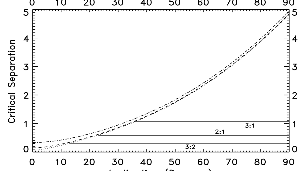
Figure 1:

Figure 2:

Figure 3:

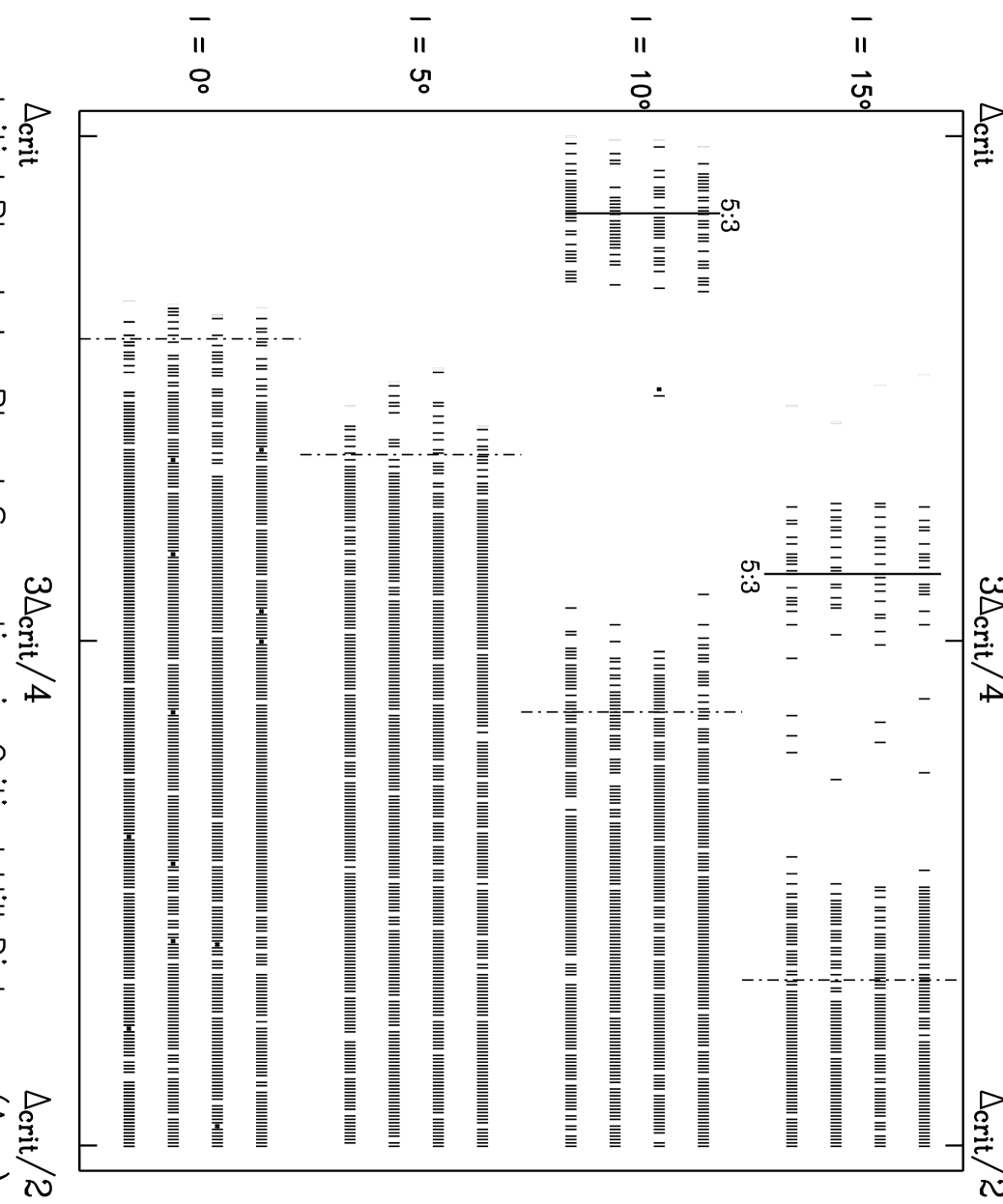
Figure 4:

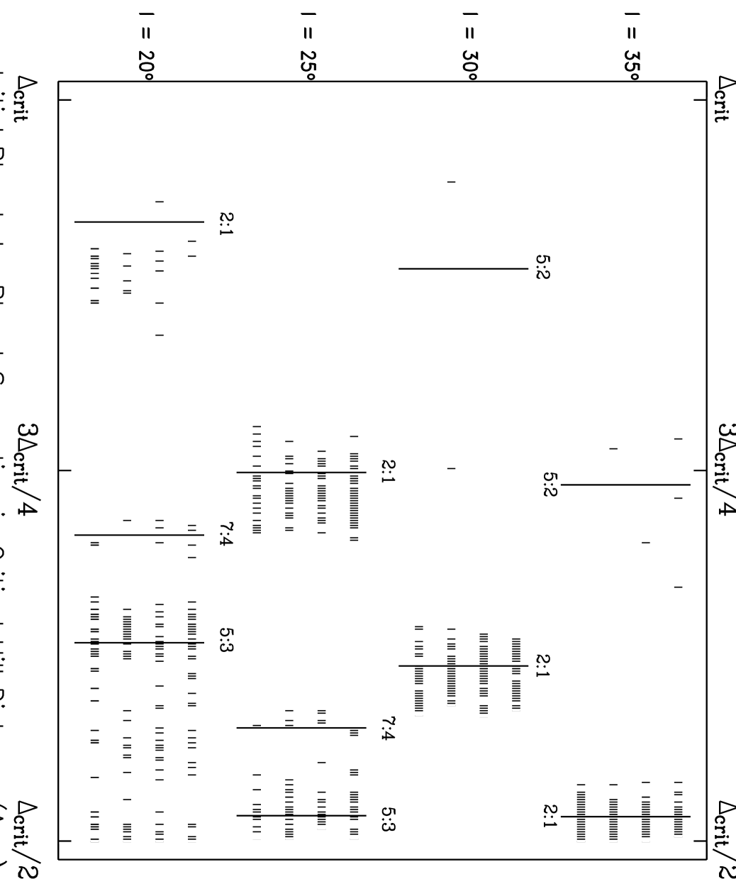
Figure 5:

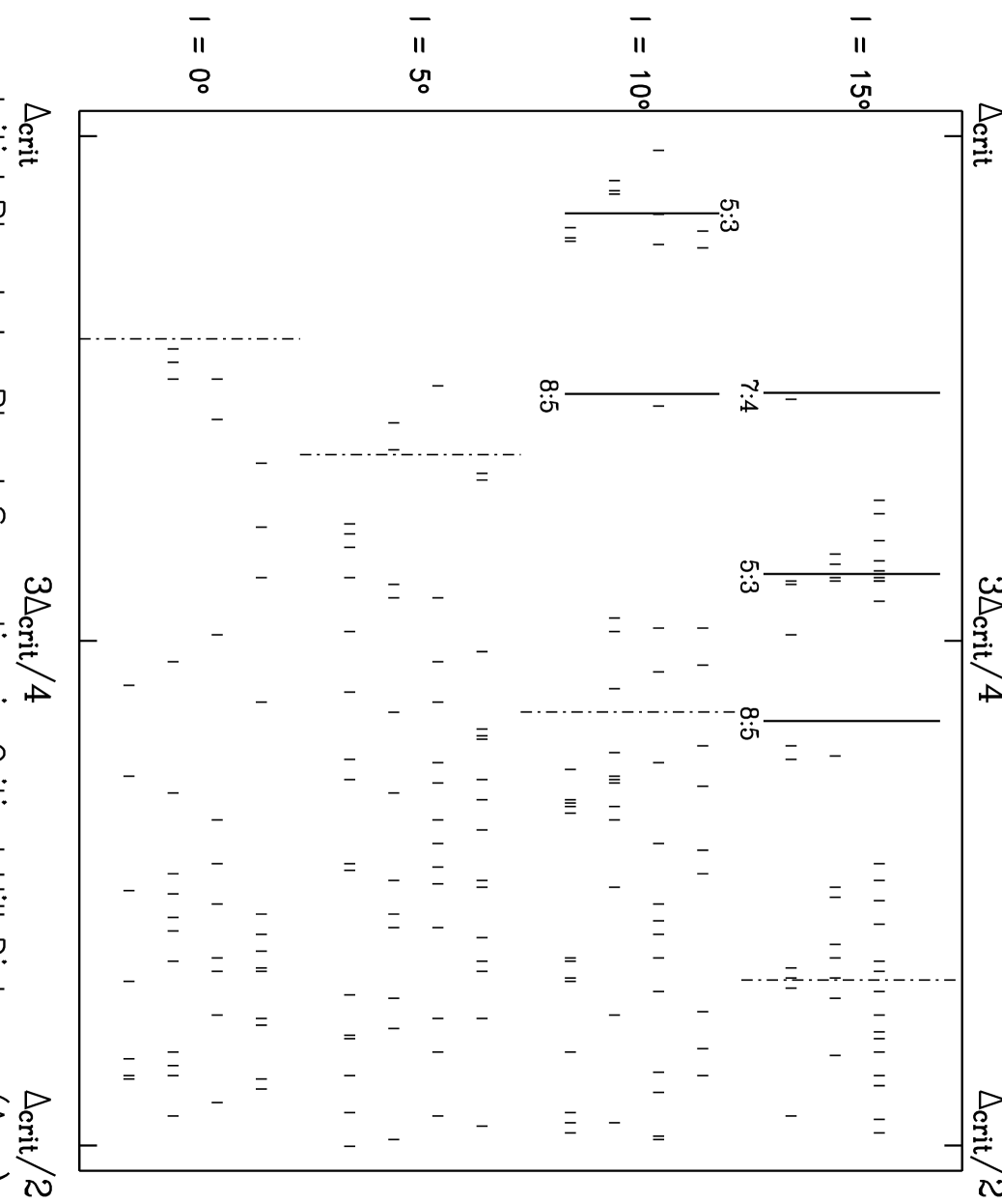
Figure 6:

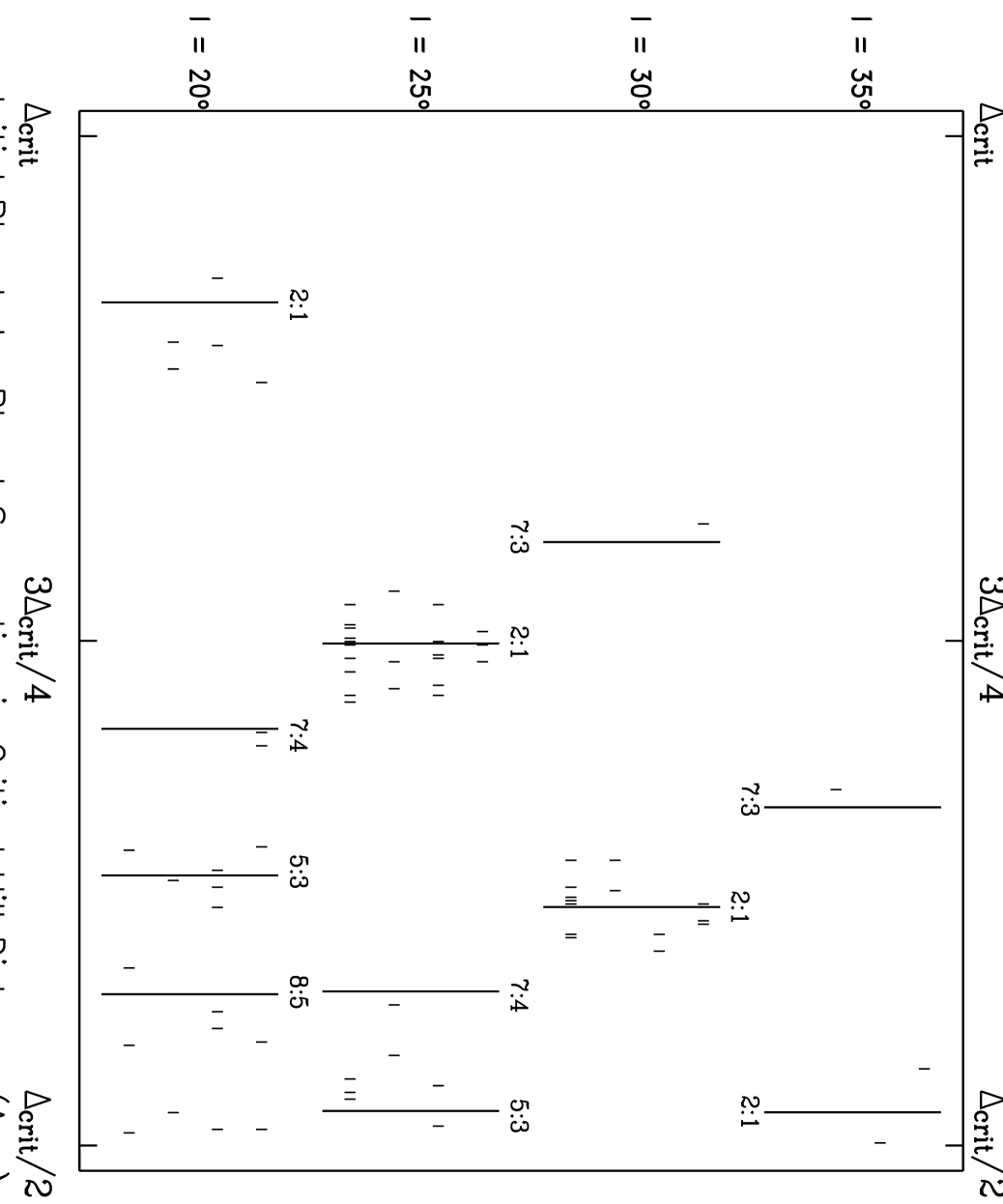
Figure 7:

Figure 8:

Figure 9:

Figure 10:

Figure 11:

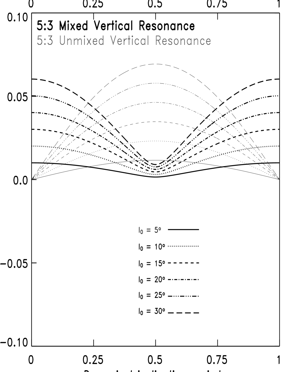
Figure 12:

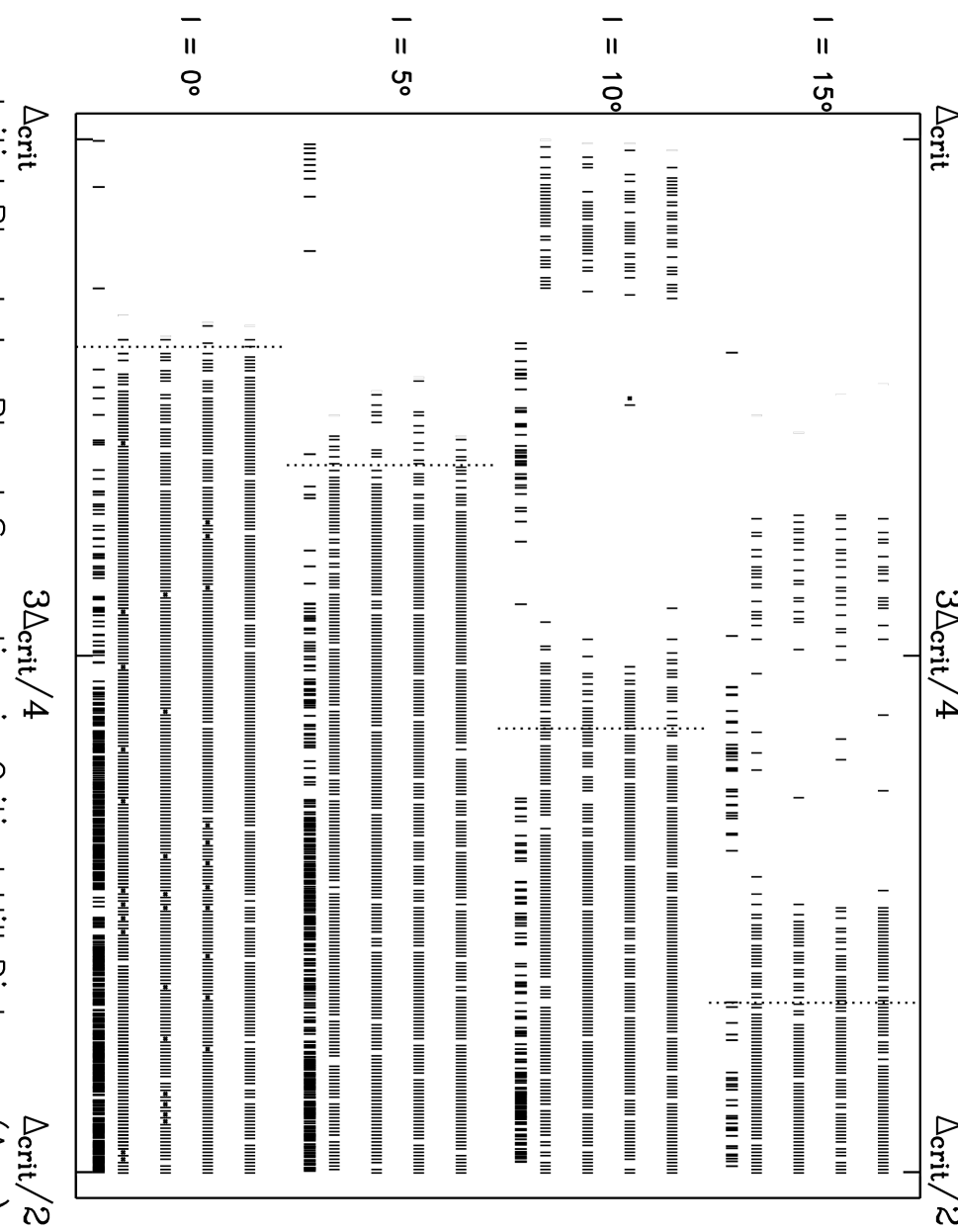
Figure 13:

Figure 14:

Figure 15: