Cosmic-Ray Background Flux Model based on a Gamma-Ray Large-Area Space Telescope Balloon Flight Engineering Model

Abstract

Cosmic-ray background fluxes were modeled based on existing measurements and theories and are presented here. The model, originally developed for the Gamma-ray Large Area Space Telescope (GLAST) Balloon Experiment, covers the entire solid angle (${\rm 4\pi~{}sr}$), the sensitive energy range of the instrument (${\rm\sim 10~{}MeV~{}to~{}100~{}GeV}$) and abundant components (proton, alpha, $e^{-}$, $e^{+}$, $\mu^{-}$, $\mu^{+}$ and gamma). It is expressed in analytic functions in which modulations due to the solar activity and the Earth geomagnetism are parameterized. Although the model is intended to be used primarily for the GLAST Balloon Experiment, model functions in low-Earth orbit are also presented and can be used for other high energy astrophysical missions. The model has been validated via comparison with the data of the GLAST Balloon Experiment.

1 Introduction

In high energy gamma-ray astrophysics observations, it is vital to reduce the background effectively in order to achieve a high sensitivity, for the source intensity is quite low. Most of the background events are generated via an interaction between cosmic-rays and the instrument, and an accurate cosmic-ray flux model and computer simulation are necessary to develop the background rejection algorithm and evaluate the remaining background level. The model needs to cover the entire solid angle (${\rm 4\pi~{}sr}$) and the sensitive energy range of the instrument. While there are many measurements on cosmic-rays reported in literature, they are fragmentary and need to be compiled, reviewed and validated.

The Large Area Telescope (LAT) is the high-energy gamma-ray detector onboard the Gamma-ray Large Area Space Telescope (GLAST) satellite to be launched to low-Earth orbit (altitude of ${\rm\sim 550~{}km}$) in 2007 (Gehrels & Michelson, 1999). It consists of 16 towers in a 4 x 4 array. Each tower has a set of high-Z foil and Si strip pair conversion trackers (TKR) and a CsI(Tl) hodoscopic calorimeter (CAL). The towers are surrounded on the top and sides by a set of plastic scintillator anticoincidence detectors (ACD). Because the LAT will have a large active volume (${\rm 1.8~{}m\times 1.8~{}m\times 1~{}m}$), the data acquisition trigger, based on signals in three consecutive x-y pair layers of the TKR, is expected to be about 10 kHz, whereas the gamma-ray signal from a strong extraterrestrial source (e.g., Crab pulsar) is only about one per minute. In order to achieve the required sensitivity, we have to develop a “cosmic-ray proof” instrument by an optimized on-line/off-line event filtering scheme. All possible background types need to be studied in detail by beam tests and computer simulations.

To validate the basic design of LAT in a space-like environment, and collect particle incidences to be used as a background event database for LAT, a Balloon Flight Engineering Model (BFEM), representing one of 16 towers that compose the LAT, was built and launched on August 4, 2001 (Thompson et al., 2002). The instrument operated successfully and took data for about two hours during the ascent and three hours during the level flight. A Geant4-based (Agostinelli et al., 2003) simulator of BFEM was constructed for this balloon experiment. We also have developed a cosmic-ray background flux model based on existing measurements and theoretical predictions, and validated the model by comparing with the data of BFEM. The model covers the entire solid angle ($\rm 4\pi~{}sr$), a wide energy range between 10 MeV to 100 GeV and abundant components (proton, alpha, $e^{\pm}$, $\mu^{\pm}$ and gamma ray). In this paper, we present the model functions as “a working model of cosmic-ray background fluxes” for high energy astrophysical missions. Although the models are intended to be used primarily for GLAST BFEM, they are expressed in analytic functions in which modulations due to solar activity and Earth geomagnetism are parameterized, and they are easy to be applied to other balloon and satellite experiments. The models in low-Earth orbit are being used to simulate the GLAST LAT in the orbital environment and to develop background rejection algorithms.

2 Instrument and Simulator

The GLAST LAT BFEM was a reconfigured version of the Beam Test Engineering Model (BTEM) that represents one of 16 towers of the LAT and consists of ACD, TKR and CAL. The BFEM differed from BTEM in that 6 silicon tracker layers were removed and the data acquisition system was reconfigured. The BTEM was tested with $e^{-}$, $e^{+}$ and gamma beams at the Stanford Linear Accelerator Center (SLAC), and the results were published (Couto e Silva et al. (2001)). The BFEM ACD consisted of 13 segmented plastic anticoincidence scintillators to help identify the background events due to charged particles. Among them, 4 tiles were placed above the TKR and 8 on the side. In addition, one big tile was placed above 4 top tiles to cover gaps between tiles. The TKR consisted of 13 x-y layers of Si strip detectors (SSDs) of $400\mu{\rm m}$ thickness to measure particle tracks and 11 lead foils to convert gamma-rays. The area of SSDs was $\rm 32\ cm\times 32\ cm$ for each layer, but the top 5 x-y pairs had smaller area. Among 11 lead foils, the top 8 were 3.6% radiation length thick, the following three were 28% radiation length thick, and the last two x-y layers had no lead converter. The instrument trigger was provided by hits in three x-y pairs in-a-row (six-fold coincidence). The CAL consisted of 80 CsI crystals hodoscopically laid out (eight layers of 10 logs in x or y directions) and measured energy deposit and shower profile. A set of four plastic scintillators called eXternal Gamma-ray Target (XGT) was mounted above the instrument to tag cosmic-ray interactions in the scintillators and constrain the gamma-ray origin. The four detector components, readout electronics and support structures were mounted in a Pressure Vessel (PV) because not all of the electronics and data recorders were designed to be operated in vacuum.

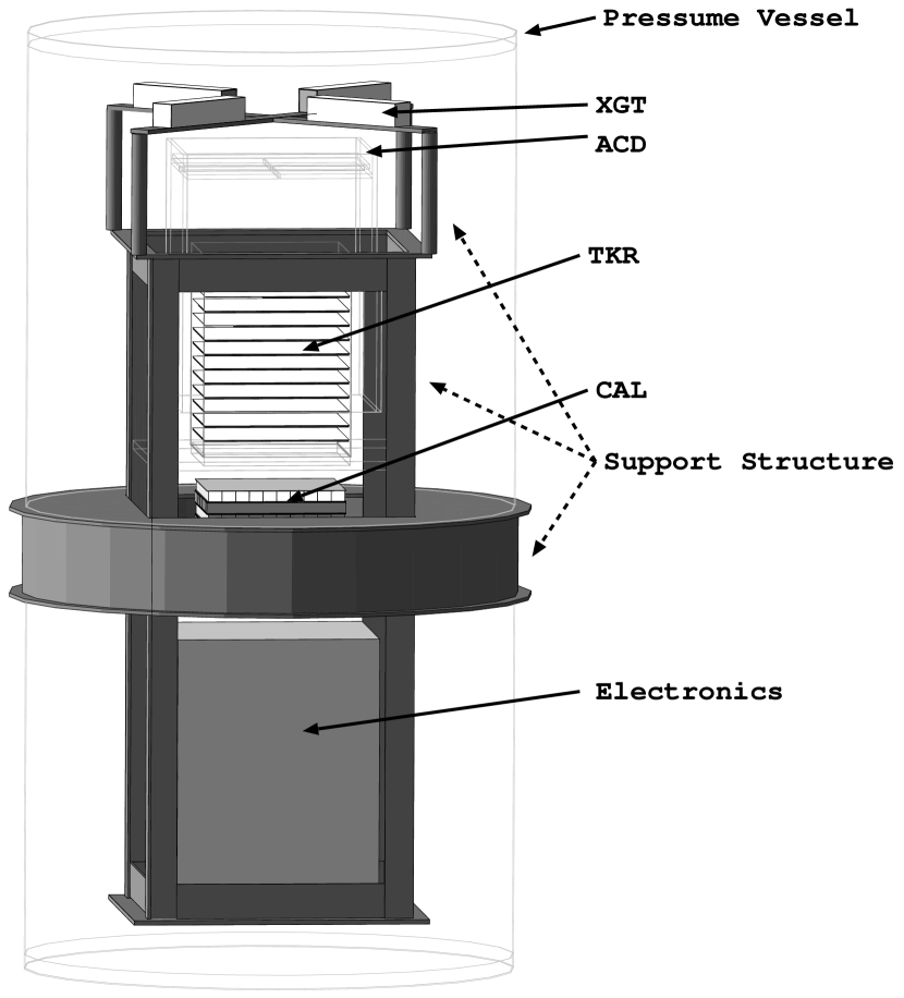
Figure 1: The geometry of the BFEM in Geant4 simulator.

We developed a Monte-Carlo simulation program of the BFEM with a Geant4 toolkit. The geometry of the BFEM implemented in the simulator is shown in Figure 1: support structures and the pressure vessel as well as detectors were implemented. Standard electromagnetic processes, hadronic interactions and decay processes were simulated. Cutoff length (range threshold of secondary particles to be generated) was set at $10\mu m$ in TKR and 1 mm for other regions. We utilized Geant4 ver 5.1 with patch 01.

3 Cosmic-Ray Background Flux Models

Cosmic-rays in or near the Earth atmosphere consist of the primary and the secondary components. The primary cosmic-rays are generated in and propagate through extraterrestrial space. The main component is known to be protons. When primary particles penetrate into the air and interact with molecules, they produce relatively low-energy particles, i.e., secondary cosmic-rays. The first step in building a working model of cosmic-ray fluxes is to represent the existing measurements and theoretical predictions by analytic functions. Below we describe the model functions particle by particle. Data are very scarce or absent for large zenith angle and low energy, and expected uncertainties are also mentioned.

3.1 Primary Charged Particle Spectra

Primary particles that reach the top of the atmosphere are believed to come predominantly from outside the solar system. Their spectra are known to be affected by the solar activity and Earth geomagnetic field. The spectra of the primaries in interstellar space can be modeled by a power-law in rigidity (or momentum) as

$$Unmod(E_{\rm k})=A\times\left(\frac{R(E_{\rm k})}{\rm GV}\right)^{-a}\quad,$$ (1)

where $E_{\rm k}$ and $R$ are the kinetic energy and rigidity of the particle, respectively. These particles are decelerated by solar wind as they enter the solar system and hence their flux shows anti correlation with the solar activity. To model this solar modulation, we adopted the formula given by Gleeson & Axford (1968): the modulation is expressed by an effective shift of energy as

$$Mod(E_{\rm k})=Unmod(E_{\rm k}+Ze\phi)\times\frac{\left(E_{\rm k}+Mc^{2}\right)^{2}-\left(Mc^{2}\right)^{2}}{\left(E_{\rm k}+Mc^{2}+Ze\phi\right)^{2}-\left(Mc^{2}\right)^{2}}\quad,$$ (2)

where $e$ is the magnitude of electron charge, $Z$ the atomic number of particle, $M$ the particle mass and $c$ the speed of light. A parameter $\phi$ is introduced to represent the solar modulation which varies from $\sim 550~{}{\rm MV}$ for solar activity minimum to $\sim 1100~{}{\rm MV}$ for solar activity maximum. Since the GLAST Balloon experiment took place in 2001 August, we fixed $\phi$ at 1100 MV, a typical value for solar activity maximum.

The second and much bigger modulation is introduced as the low energy cutoff due to the Earth geomagnetism. We modeled this effect based on the AMS measurements (Alcaraz et al., 2000a) in which the proton flux was measured over a wide geomagnetic latitude range. We defined the reduction factor as

$$\frac{1}{1+\left(\frac{R}{R_{\rm cut}}\right)^{-12.0}}\quad.$$ (3)

Here, $R_{\rm cut}$ is the cutoff rigidity calculated by assuming the Earth magnetic field to be of dipole shape, as

$$R_{\rm cut}=14.9\times\left(1+\frac{h}{R_{\rm Earth}}\right)^{-2.0}\times\left(\cos\theta_{\rm M}\right)^{4}\ {\rm GV}\quad,$$ (4)

where $h$ is the altitude, $R_{\rm Earth}$ the Earth radius and $\theta_{\rm M}$ the geomagnetic latitude (Zombeck, 1990; Longair, 1992). For the GLAST Balloon Experiment they were $h\sim 38$ km, $\theta_{\rm M}\sim 0.735$ rad, and $R_{\rm cut}=4.46~{}{\rm GV}$. We also referred to $e^{-}$ measurements by AMS (Alcaraz et al., 2000b) and found that electrons are less affected by Earth geomagnetism. Although the geomagnetic cutoff is expected to be the same regardless of the particle type, we gave priority to the experimental data and used

$$\frac{1}{1+\left(\frac{R}{R_{\rm cut}}\right)^{-6.0}}\quad,$$ (5)

instead of equation (3) for $e^{-}$/$e^{+}$. The reduction factor of equations (3) and (5) reproduces the cutoff seen in AMS data in $0\leq\theta_{\rm M}\leq 0.8~{}{\rm rad}$, but gives lower flux in high geomagnetic latitude region.

The primary spectrum is then expressed as

$$Primary(E_{\rm k})=Unmod(E_{\rm k}+Ze\phi)\times\frac{\left(E_{\rm k}+Mc^{2}\right)^{2}-\left(Mc^{2}\right)^{2}}{\left(E_{\rm k}+Mc^{2}+Ze\phi\right)^{2}-\left(Mc^{2}\right)^{2}}\times\frac{1}{1+\left(\frac{R}{R_{\rm cut}}\right)^{-r}}\quad,$$ (6)

where $r=12.0$ and 6.0 for proton/alpha and $e^{-}$/$e^{+}$, respectively. This model function can be used for the entire solar cycle and entire low-Earth orbit by adjusting $\phi$ and $R_{\rm cut}$. We assume the angular distribution is uniform for $0^{\circ}\leq\theta\leq\theta_{\rm c}$ and to be 0 for $\theta_{\rm c}\leq\theta\leq 180^{\circ}$, where $\theta$ is the zenith angle from vertical. The cutoff angle $\theta_{\rm c}$ is introduced to represent the Earth horizon and is $113^{\circ}$ at low-Earth orbit ($\sim 550~{}{\rm km}$). The primary flux at balloon altitude is attenuated by air and the effect is described in the following sections particle by particle. Note that the east-west effect is not taken into account for simplicity: we aim to construct models which provide the correct flux integrated over the azimuth angle.

3.2 Proton Flux

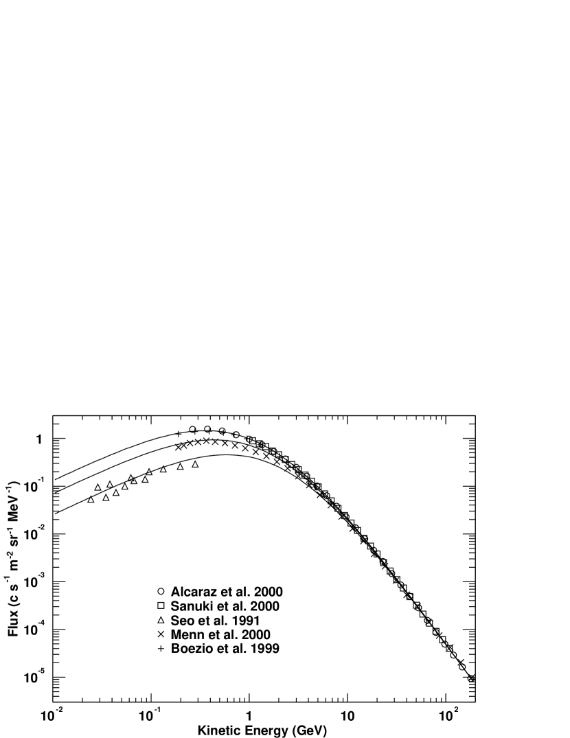
Figure 2: A compilation of measured primary proton spectra in high geomagnetic latitude region. Three lines are our model functions (equation 2) with $\phi$=650 MV (upper line), 800 MV (middle line), and 1100 MV(lower line).

Recent measurements by BESS (Sanuki et al., 2000) and AMS (Alcaraz et al., 2000a, c) provided us with an accurate spectrum of primary protons. These data were taken in similar parts of the solar cycle (June/July, 1998), and we expect that the solar modulation parameters are similar between them. BESS measured the proton flux at an altitude of 37 km near the geomagnetic north pole and evaluated the spectrum at the top of the atmosphere, which was not much affected by the geomagnetic cutoff. AMS measured the flux at various positions on Earth in energies below and above the geomagnetic cutoff at an altitude close to low-Earth orbit (380 km). Above the geomagnetic cutoff the two measurements agree up to about 50 GeV and differ less than 10% between 50 and 100 GeV (Alcaraz et al., 2000c). Their data can be modeled well by equation (2) with $\phi=650~{}{\rm MV}$, $A=23.9~{}{\rm c~{}s^{-1}~{}m^{-2}~{}sr^{-1}~{}MeV^{-1}}$ and $a=2.83$. Other experiments (Seo et al., 1991; Boezio et al., 1999a; Menn et al., 2000) can also be represented by the model if the solar modulation parameter $\phi$ is adjusted to an appropriate solar cycle (see Figure 2).

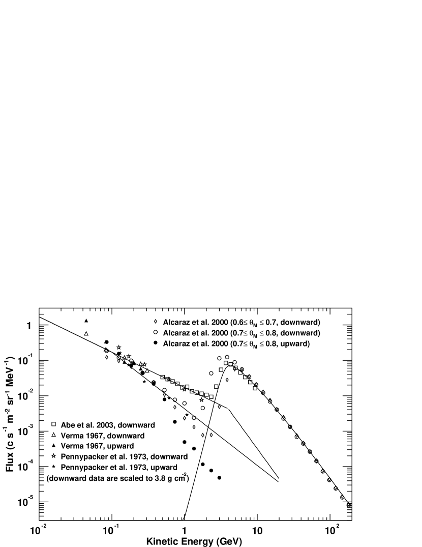
Figure 3: The proton vertically downward/upward spectra at $R_{\rm cut}\sim 4.5$ GV observed by balloon experiments and AMS. Atmospheric depths are $\rm 4.6\ g\ cm^{-2}$, $\rm 4\ g\ cm^{-2}$, and $\rm 5\ g\ cm^{-2}$ for data by Abe et al. (2003), data by Verma (1967), and data by Pennypacker (1973), respectively. Solid lines are model functions of primary and secondary proton spectra for GLAST Balloon Experiments.

The flux at a balloon altitude suffers a small attenuation due to interactions with air. The nuclear interaction length in air is $90.0~{}{\rm g~{}cm^{-2}}$, and the probability for vertically-downward protons to reach the altitude of GLAST BFEM (atmospheric depth was $3.8~{}{\rm g~{}cm^{-2}}$) is 95.8%. For protons of oblique direction, we calculated the atmospheric depth in line-of-sight by assuming the trajectory to be straight. Then the effective atmospheric depth scales as $\frac{1}{\cos\theta}$ down to $\cos\theta=0.2$ and is $138~{}{\rm g~{}cm^{-2}}$ for the horizontal direction, by assuming the scale height of the air above the altitude of the payload (at $\sim 38~{}{\rm km}$) to be 7.6 km, a typical value in the U.S. Standard Atmosphere. Below the horizon the flux is assumed to be 0. Our primary proton spectral model function (equation 6 with 4% air attenuation) with adjustment for the geomagnetic cutoff is shown in Figure 3 with AMS data taken at similar geomagnetic latitude region.

In energy ranges below the geomagnetic cutoff, there are secondary particles produced in the Earth’s atmosphere by interactions of primaries. The secondary proton spectra at satellite altitude was measured by AMS in a wide geomagnetic latitude region, showing strong dependence on the geomagnetic cutoff. We represent their data, region by region, by a broken power-law or cutoff power-law model. The formula of the broken power-law is,

$$\begin{array}[]{ll}F_{0}\times\left(\frac{E_{\rm k}}{\rm 100~{}MeV}\right)^{-a}&({\rm 100~{}MeV}\leq E_{\rm k}\leq E_{\rm bk})\\ F_{0}\times\left(\frac{E_{\rm bk}}{\rm 100~{}MeV}\right)^{-a}\times\left(\frac{E_{\rm k}}{E_{\rm bk}}\right)^{-b}&(E_{\rm bk}\leq E_{\rm k})\\ \end{array}\quad,$$ (7)

and that of the cutoff power-law model is

$$\begin{array}[]{ll}F_{1}\times\left(\frac{E_{\rm k}}{\rm GeV}\right)^{-a}\times e^{-\left(\frac{E_{\rm k}}{E_{\rm c}}\right)^{-a+1}}&({\rm 100~{}MeV}\leq E_{\rm k})\\ \end{array}\quad.$$ (8)

Below 100 MeV, we found no data and assume a power-law spectrum with index of -1:

$$\begin{array}[]{ll}F_{0}\times\left(\frac{E_{\rm k}}{\rm 100~{}MeV}\right)^{-1}&({\rm 10~{}MeV}\leq E_{\rm k}\leq{\rm 100~{}MeV})\\ \end{array}\quad.$$ (9)

Below a few $\times$ 10 MeV, there is no probability for protons to trigger BFEM/LAT, hence the spectral model below 100 MeV (equation 9) does not affect the data very much. We tabulated the model parameters to describe the AMS data in Table 1. In low geomagnetic latitude regions ($\theta_{\rm M}\leq 0.6$) the downward and upward spectra are identical, indicating that protons are confined locally by the geomagnetic field. The particle direction is expected to be randomized, and we adopt a uniform angular distribution. For $\theta_{\rm M}\geq 0.6$, we assume a uniform zenith angle dependence in the upper and lower hemispheres, for we lack experimental data about angular dependence. Flux in the horizontal direction is uncertain, and we leave it discontinuous. Analysis of the BFEM data ($\S~{}5$) showed that horizontal particles ($\theta=90^{\circ}\pm 20^{\circ}$) have little chance to trigger the BFEM. The 3-in-a-row trigger is improbable for the narrow geometry of this single tower.

The secondary proton spectrum at balloon altitude is not necessarily the same as that in low-Earth orbit, for the Larmor radius of a typical secondary proton is much smaller than the satellite altitude: for example, the radius of a 1 GeV proton is 100 km for average Earth magnetic field of 0.3 gauss. Hence we must refer to existing balloon measurements. The spectra measured at $R_{\rm cut}\sim 4.5$ GV at atmospheric depth similar to our experiment ($\rm 3.8\ g\ cm^{-2}$) are collected in Figure 3 (Verma, 1967; Pennypacker et al., 1973; Abe et al., 2003). Although the flux differs from experiment to experiment, vertically-downward flux at ${\rm\sim 4\ g\ cm^{-2}}$ is much higher than that measured by AMS (at 380 km): they could be represented as

$$0.17\times\left(\frac{E_{\rm k}}{\rm 100~{}MeV}\right)^{-1.0}\ {\rm c\ s^{-1}\ m^{-2}\ sr^{-1}\ MeV^{-1}}\quad,$$ (10)

in 10 MeV–4 GeV. Above the geomagnetic cutoff, we assume that the secondary proton flux follows a power-law function of $\left(\frac{E_{\rm k}}{\rm GeV}\right)^{-2.83}$, i.e., that of the primary. Note that the downward flux is known to be proportional to the atmospheric depth (Verma, 1967; Abe et al., 2003), and balloon data in Figure 3 were already scaled to $3.8~{}{\rm g~{}cm^{-2}}$. On the other hand, upward flux does not depend on the atmospheric depth very much (e.g., Verma 1967) and we modeled the data with the following formulas. They are

$$0.17\times\left(\frac{E_{\rm k}}{\rm 100~{}MeV}\right)^{-1.6}\ {\rm c\ s^{-1}\ m^{-2}\ sr^{-1}\ MeV^{-1}}\quad,$$ (11)

for energy above 100 MeV and

$$0.17\times\left(\frac{E_{\rm k}}{\rm 100~{}MeV}\right)^{-1.0}\ {\rm c\ s^{-1}\ m^{-2}\ sr^{-1}\ MeV^{-1}}\quad,$$ (12)

for energy below 100 MeV. As can be seen from Figure 3, secondary fluxes measured by balloon experiments are mutually inconsistent within a factor of 2. Hence our model inherits this much uncertainty.

The angular distribution of the secondary cosmic-ray flux has been measured in several balloon and rocket experiments. While substantial build-up of the flux near the Earth horizon has been reported in several experiments (Van Allen & Gangnes, 1950a, b; Singer, 1950), its functional form is not well determined. For small zenith angles, the secondary proton downward flux is expected to be proportional to the atmospheric depth in line-of-sight, and we multiply the flux by $\frac{1}{\cos\theta}$. The flux is expected to be saturated near the horizon and we use a constant factor of 2 for $60^{\circ}\leq\theta\leq 90^{\circ}$. For upward flux, we assume the same angular dependence as a function of nadir angle instead of zenith angle. Again the flux disconnects at horizon due to uncertainty.

3.3 Alpha Particle Flux

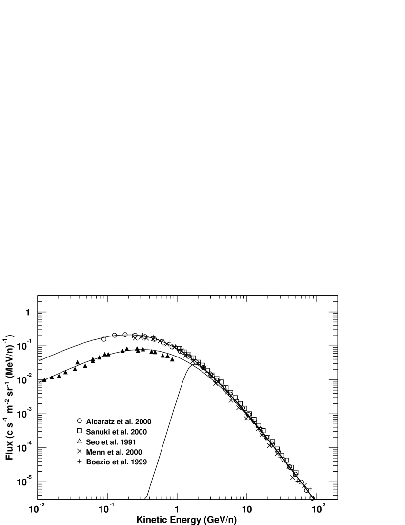
Figure 4: The alpha primary flux observed in high geomagnetic region. Our model functions (equation 2) of $\phi$=650 MV (upper line) and 1100 MV (lower line) are also shown. Solid line with a cutoff below a few GeV is the model function for GLAST BFEM (equation 6).

We adopted the AMS and BESS data to model the alpha particle spectrum. The two experiments are consistent with each other to $\sim$10 % (Alcaraz et al., 2000d), giving $A=1.50\ {\rm c\ s^{-1}\ m^{-2}\ sr^{-1}\ MeV^{-1}}$, $a=2.77$ and $\phi=650~{}{\rm MV}$ for equation 2. Other experiments (Seo et al., 1991; Boezio et al., 1999a; Menn et al., 2000) can also be represented well by adjusting the solar modulation parameter $\phi$ (Figure 4). We did not take the secondary component into account, for the flux is more than three orders of magnitude lower than the primary, as shown by Alcaraz et al. (2000d). For the GLAST balloon experiment, we used equation 3 with ${\rm\phi=1100\ MV}$ and $R_{\rm cut}=4.46\ {\rm GV}$. The zenith angle dependence and the attenuation by air are assumed to be the same as that of proton primaries.

3.4 Electron and Positron Flux

The fluxes of cosmic-ray electrons and positrons are modeled in 3 components: the primary, the secondary downward and the secondary upward fluxes.

Unlike proton and alpha primaries, no single experiment has measured cosmic primary electron and positron fluxes over a wide energy range. We referred to a compilation of measurements by Webber (Webber, 1983; Longair, 1992) and used the power-law fit given there, i.e.,

$$Unmod(E_{\rm k})=0.7\times\left(\frac{R(E_{\rm k})}{\rm GV}\right)^{-3.3}\ {\rm c\ s^{-1}\ m^{-2}\ sr^{-1}\ MeV^{-1}}~{}.$$ (13)

A recent review of measurements by Moskalenko & Strong (1998) gave a consistent spectrum above 10 GeV. The positively charged fraction, interpreted as $\frac{e^{+}}{e^{-}+e^{+}}$, has been measured by several experiments. Among them, Golden et al. (1994) obtained the fraction to be a constant, $0.078\pm 0.016$, between 5 GeV and 50 GeV. We adopted their results and modeled the interstellar electron spectrum to be equation 1 with $A=0.65\ {\rm c\ s^{-1}\ m^{-2}\ sr^{-1}\ MeV^{-1}}$ and $a=3.3$. The spectrum of the primary positrons takes the same form except for the normalization factor. Like proton and alpha primaries, the angular distribution is assumed to be uniform and independent of zenith angle $\theta$ for $\theta\leq\theta_{\rm c}$ and zero for $\theta\geq\theta_{\rm c}$, where $\theta=0^{\circ}$ corresponds to particle going toward the nadir. The solar and geomagnetic modulation parameters for the GLAST Balloon Experiment are $\phi=1100\ {\rm MV}$ and $R_{\rm cut}=4.46\ {\rm GV}$. To model the $e^{-}$/$e^{+}$ primary flux for our experiment, we also need to take into account the energy loss due to the ionization and bremsstrahlung in the atmosphere. For vertically downward particles it is calculated to be $e^{-\frac{\rm 3.8~{}g~{}cm^{-2}}{\rm 36.6~{}g~{}cm^{-2}}}=0.90$, where ${\rm 36.6~{}g~{}cm^{-2}}$ is the radiation length of air. This energy loss gives the same spectral shape but smaller normalization by a factor of 1.42. We calculated the atmospheric depth in the line-of-sight as a function of zenith angle in the same way as that for proton and alpha primaries, and took the energy loss into account.

Secondary cosmic ray electrons and positrons are generated in two parts, a downward-moving component and an upward-moving one. To model them at a satellite altitude, we referred to the AMS data and represented them with a power-law model:

$$\begin{array}[]{ll}F_{0}\times\left(\frac{E_{\rm k}}{\rm 100~{}MeV}\right)^{-a}&({\rm 100~{}MeV}\leq E_{\rm k})\\ \end{array}\quad,$$ (14)

or a broken power-law model (equation 7), or a power-law model with a hump:

$$\begin{array}[]{ll}F_{0}\times\left(\frac{E_{\rm bk}}{\rm 100~{}MeV}\right)^{-a}+F_{1}\times\left(\frac{E_{\rm k}}{\rm GeV}\right)^{b}\times e^{-\left(\frac{E_{\rm k}}{E_{\rm c}}\right)^{b+1}}&({\rm 100~{}MeV}\leq E_{\rm k})\\ \end{array}\quad.$$ (15)

Below 100 MeV we found no data and use the power-law model with a spectral index of -1, i.e., equation 9. Again there is no probability for $e^{-}/e^{+}$ to cause trigger below 10 MeV. The model functions are tabulated in Table 2: in near geomagnetic equator, $e^{+}$ flux is much higher than that of $e^{-}$. We use the same flux models for downward and upward component, since AMS did not detect significant difference between them. As for proton secondaries, a uniform angular distribution is assumed in upper and lower hemispheres.

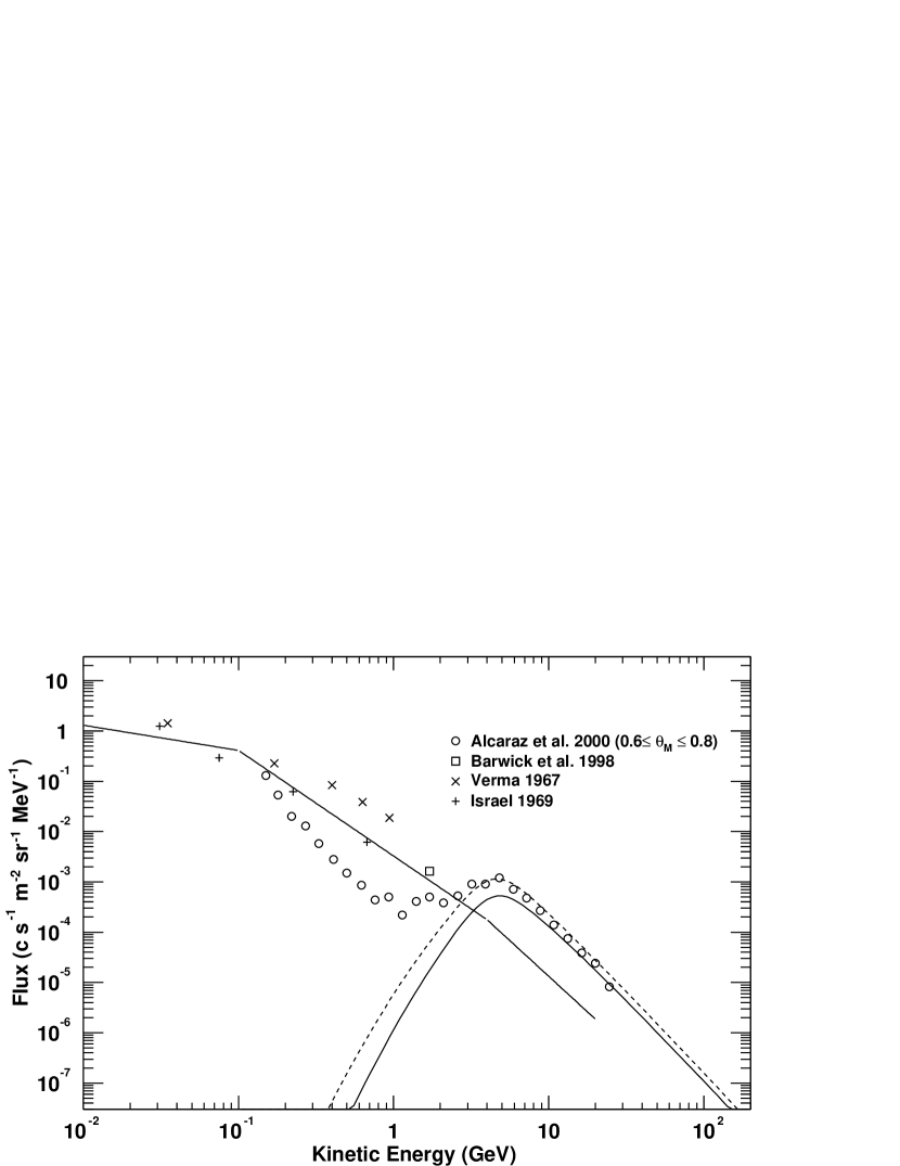
Figure 5: Electron vertically downward spectrum at $R_{\rm cut}\sim 4.5$ GV measured by balloon experiments and AMS. Model functions for the GLAST Balloon Experiments are shown by solid lines. Dotted line is the primary spectral model with no air attenuation and of $\phi=650~{}{\rm MV}$, a value for AMS observation.

Most of the existing balloon measurements of secondary electron flux at around $R_{\rm cut}=4.5\ {\rm GV}$ (Verma, 1967; Israel, 1969; Barwick et al., 1998) were rather old and inconsistent with each other, as shown in Figure 5. However, they consistently show much higher and flatter spectra than that of AMS. We therefore referred to balloon measurements and adopted a higher and flatter spectral model for the GLAST Balloon Experiment. The vertically downward spectrum is

$$0.41\times\left(\frac{E_{\rm k}}{\rm 100~{}MeV}\right)^{-2.1}\ {\rm c\ s^{-1}\ m^{-2}\ sr^{-1}\ MeV^{-1}}\quad,$$ (16)

for 100 MeV–4 GeV and

$$0.41\times\left(\frac{E_{\rm k}}{\rm 100~{}MeV}\right)^{-0.5}\ {\rm c\ s^{-1}\ m^{-2}\ sr^{-1}\ MeV^{-1}}\quad,$$ (17)

in energy 10–100 MeV. The flux above the geomagnetic cutoff is expected to follow the functional form of proton primaries ($E_{\rm k}^{-2.83}$). Upward flux has been measured by DuVernois et al. (2001) in 1.0–2.4 GeV and is similar to that of downward, and we used the same spectral model for both downward and upward for simplicity. We did not find data at large zenith angle, and assume the same angular distribution as that for proton secondaries.

Although AMS (Alcaraz et al., 2000b) observed an overabundance of positrons relative to electrons in the low geomagnetic latitude region, fluxes of these two particles are almost identical in the region of $\theta_{\rm M}\geq 0.6$, as shown in Table 2. A recent balloon measurement by Barwick et al. (1998) also showed that the positron fraction is nearly 50% at $R_{\rm cut}=4.5\ {\rm GV}$. We therefore used the same spectral shape and flux for positron secondaries. Note that the data points of balloon experiments referenced, where only the flux of $e^{-}+e^{+}$ is given, have been divided by 2 to convert to the $e^{-}$ flux in Figure 5.

3.5 Gamma-ray Flux

As for particles at balloon altitudes, the gamma-ray flux consists of primary and secondary components. The primary component is of extraterrestrial origin and the intensity is attenuated by air at balloon altitude. Secondaries are produced by the interaction between cosmic-ray particles and the atmospheric molecules, and the intensity of the downward component depends on the residual atmospheric depth.

3.5.1 Primary Gamma-ray Flux

We modeled the extragalactic diffuse gamma-rays measured by several gamma-ray satellites, as compiled by Sreekumar et al. (1998). Above 1 MeV, the spectrum can be expressed by a power-law function of

$$40.0\times\left(\frac{E_{\rm k}}{\rm MeV}\right)^{-2.15}~{}{\rm c~{}s^{-1}~{}m^{-2}~{}sr^{-1}~{}MeV^{-1}}~{}.$$ (18)

The zenith-angle dependence is the same as those of proton/alpha/$e^{\pm}$ primaries. For energies where GLAST BFEM has sensitivity for gamma rays ($E_{k}\geq 1~{}{\rm MeV}$), the primary flux is lower than that of secondary downward gamma by more than an order of magnitude. We therefore do not take into account the gamma primary component in the following analysis of BFEM data (§ 5).

3.5.2 Secondary Gamma-ray Flux

Secondary gamma-rays are produced either by interactions of cosmic-ray hadrons or bremsstrahlung of $e^{\pm}$ with nuclei in the atmosphere. The spectrum has been measured by several satellite and balloon experiments (Thompson, 1974; Imhof, Nakano, & Reagan, 1976; Ryan et al., 1979; Kur’yan et al., 1979; Shönfelder et al., 1980; Daniel & Stephens, 1974). For residual atmosphere less than $\rm 100\ g\ cm^{-2}$, the vertically-downward gamma-ray flux is known to be proportional to the atmospheric depth, whereas the upward flux remains almost constant (Thompson, 1974). Observations at Palestine of the vertically downward spectrum at the atmospheric depth of ${\rm 2.5~{}g~{}cm^{-2}}$ are compiled in Shönfelder et al. (1980) and Daniel & Stephens (1974), showing consistent results. We multiplied their data by $\frac{3.8}{2.5}$ to scale them to the residual atmosphere of $\rm 3.8\ g\ cm^{-2}$, the value for the GLAST Balloon Experiment, and modeled the spectrum as follows: For 1-1000 MeV, it is

$$250\times\left(\frac{E_{\rm k}}{\rm MeV}\right)^{-1.7}+1.14\times 10^{5}\times\left(\frac{E_{\rm k}}{\rm MeV}\right)^{-2.5}\times e^{-\left(\frac{E_{\rm k}}{E_{\rm c}}\right)^{-1.5}}\ {\rm c\ s^{-1}\ m^{-2}\ sr^{-1}\ MeV^{-1}}\quad,$$ (19)

where $E_{\rm c}=120\ {\rm MeV}$. For 1–100 GeV, the spectrum is

$$2.15\times 10^{4}\times\left(\frac{E_{\rm k}}{\rm MeV}\right)^{-2.2}\ {\rm c\ s^{-1}\ m^{-2}\ sr^{-1}\ MeV^{-1}}\quad.$$ (20)

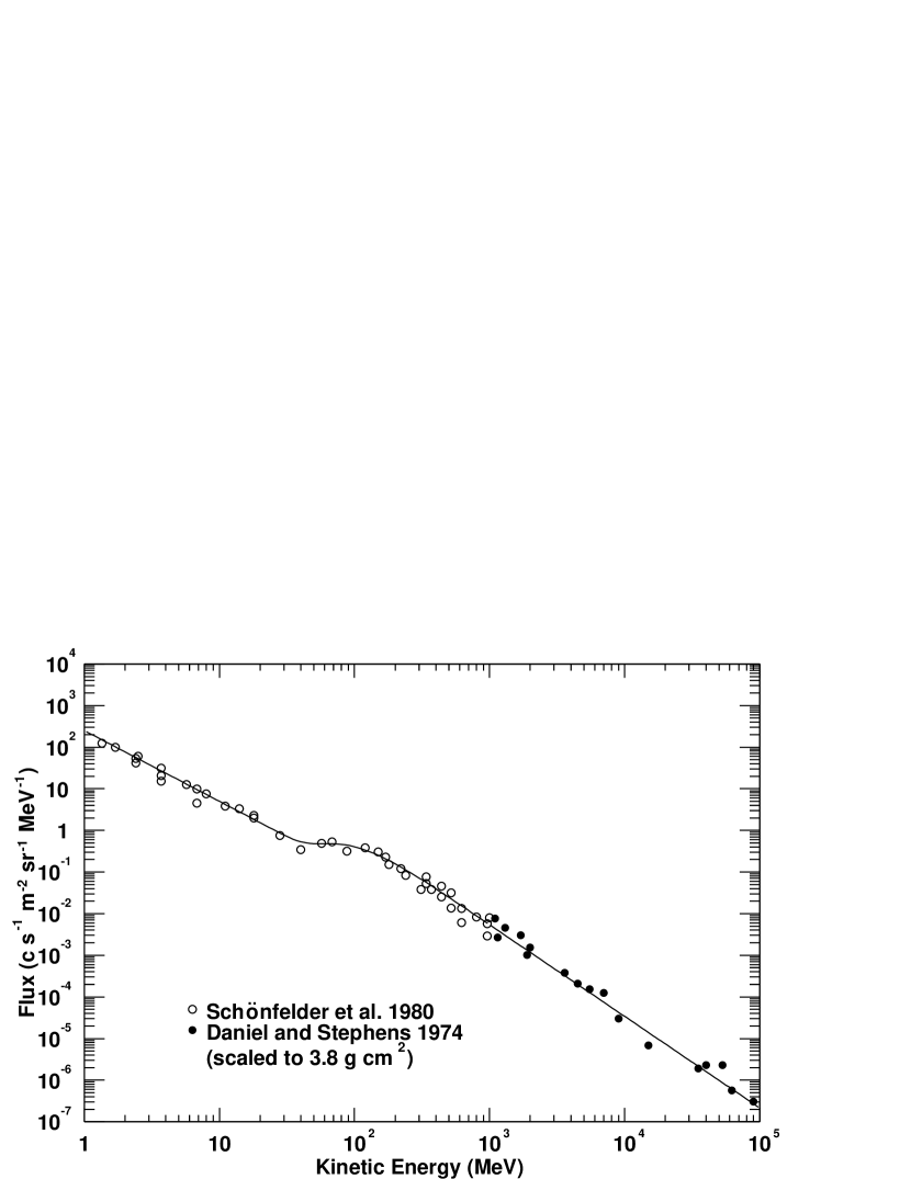
Figure 6: Vertically downward atmospheric gamma-ray spectrum. Spectral model is shown by solid line and reference data by filled and open circles.

The composite spectrum is shown with reference data in Figure 6. Note that we do not expect this component in satellite orbit.

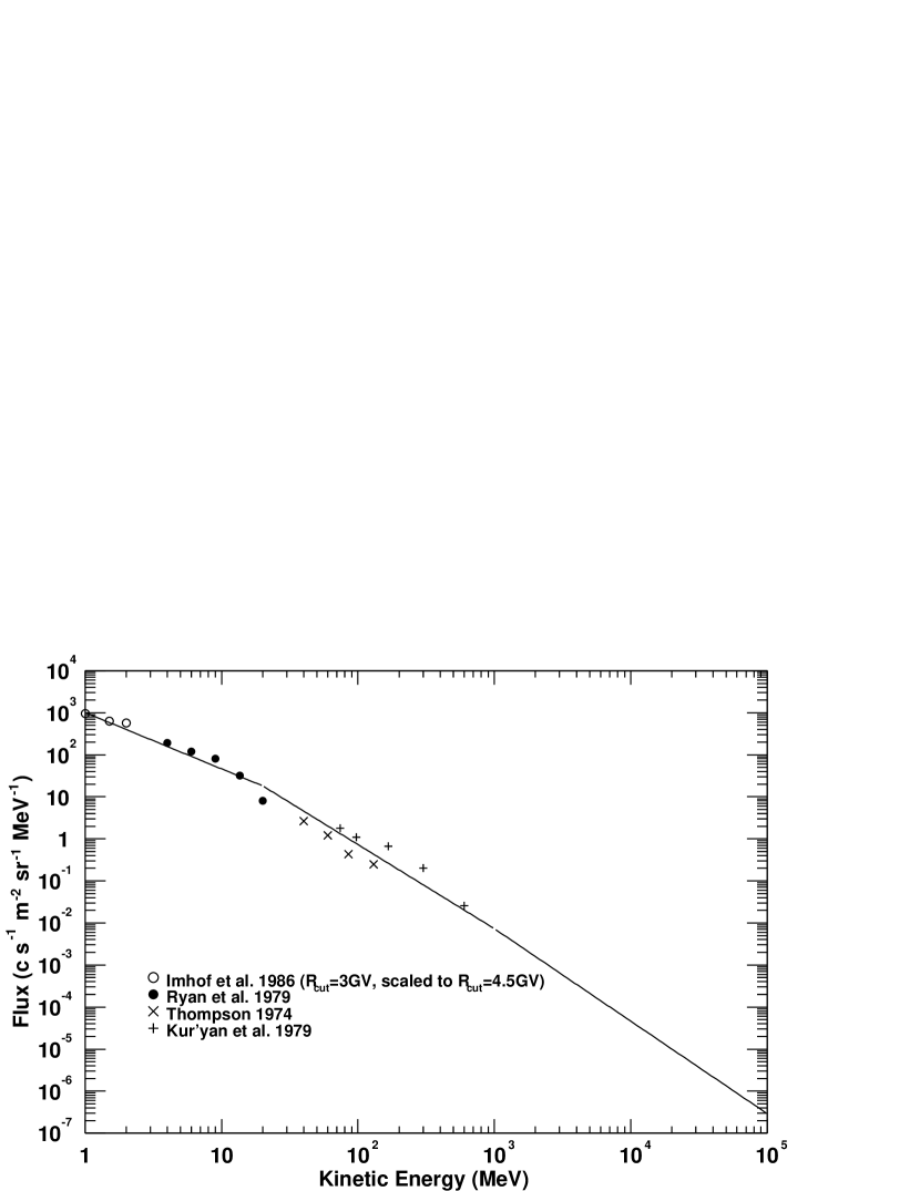
Figure 7: Vertically upward gamma-ray spectral model with reference data.

For the vertically-upward component, only a few data are available (Thompson, 1974; Imhof, Nakano, & Reagan, 1976; Ryan et al., 1979; Kur’yan et al., 1979) as collected in Figure 7. We found data taken at Palestine, Texas ($R_{\rm cut}\sim 4.5\ {\rm GV}$) down to a few MeV, whereas we found none below a few MeV: so we substituted with data by Imhof, Nakano, & Reagan (1976) at $R_{\rm cut}=3\ {\rm GV}$. The flux depends on cut-off rigidity, as discussed in Kur’yan et al. (1979): they measured the flux of vertically-upward gammas above 80 MeV, for which GLAST LAT/BFEM has high sensitivity, in $R_{\rm cut}$ of 4–17.5 GeV, and showed that the flux anticorrelates the cutoff rigidity as ${R_{\rm cut}}^{-1.13}$. Thompson, Simpson & Özel (1981) confirmed the dependence by comparing the gamma-ray intensity above 35 MeV at equator and at $R_{\rm cut}\sim 4.5~{}{\rm GeV}$. We adopted their results and scaled the flux at $R_{\rm cut}=3\ {\rm GV}$ by a factor of $\left(\frac{4.5}{3.0}\right)^{-1.13}=0.63$ to take the dependence into account. The composite spectrum for vertically upward flux seems to be represented well by two power-law functions: for 1–20 MeV, it is

$$1010\times\left(\frac{E_{\rm k}}{\rm MeV}\right)^{-1.34}\ {\rm c\ s^{-1}\ m^{-2}\ sr^{-1}\ MeV^{-1}}\quad,$$ (21)

and for 20–1000 MeV,

$$7290\times\left(\frac{E_{\rm k}}{\rm MeV}\right)^{-2.0}\ {\rm c\ s^{-1}\ m^{-2}\ sr^{-1}\ MeV^{-1}}\quad.$$ (22)

Above 1 GeV we could not find data and adopted the same spectral index as that of downward gamma rays ($E^{-2.2}$). Then, the spectrum in 1–1000 GeV is expressed as

$$2.9\times 10^{4}\times\left(\frac{E_{\rm k}}{\rm MeV}\right)^{-2.2}\ {\rm c\ s^{-1}\ m^{-2}\ sr^{-1}\ MeV^{-1}}\quad.$$ (23)

The spectral model with reference data points is given in Figure 7. As can be seen from the figure, observations are very scarce and give inconsistent results with each other. We regard that the uncertainty is a factor of 3.

3.5.3 Zenith Angle Dependence of Secondary Gamma Rays

Angular dependence of the secondary gamma-ray flux has been measured by some authors (Thompson, 1974; Shönfelder et al., 1977) and is known to depend strongly on zenith angle. We constructed the model function referring to Shönfelder et al. (1977), where they measured the flux in 1.5–10 MeV region at $\rm 2.5\ {\rm g\ cm^{-2}}$. We multiplied their data between $0^{\circ}\leq\theta<90^{\circ}$ (i.e., downward component) by 3.8/2.5 to correct the atmospheric depth, and expressed the relative flux as

$$\begin{array}[]{ll}\frac{1}{\cos\theta}&(0^{\circ}\leq\theta\leq 60^{\circ})\\ 0.367\times e^{1.618\theta}&(60^{\circ}\leq\theta\leq 90^{\circ})\\ 8.71\times 10^{-3}\times e^{4.0\theta}&(90^{\circ}\leq\theta\leq 115^{\circ})\\ 25760\times e^{-3.424\theta}&(115^{\circ}\leq\theta\leq 140^{\circ})\\ 6&(140^{\circ}\leq\theta\leq 180^{\circ})\\ \end{array}\quad.$$ (24)

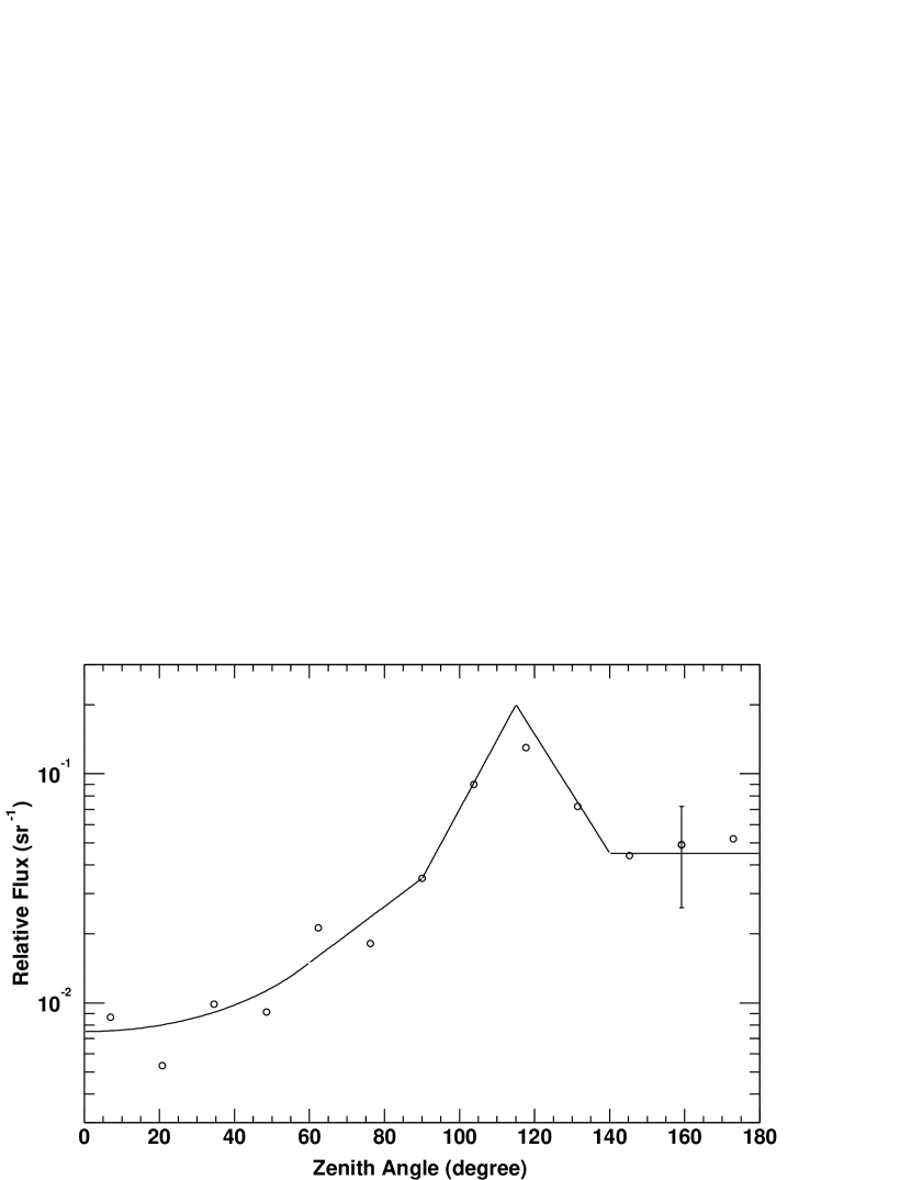
Figure 8: Zenith angle dependence of the gamma secondary flux measured by Shönfelder et al. (1977) in 1.5–10 MeV and model functions. Data points of downward are multiplied by a factor of 3.8/2.5 to correct the atmospheric depth dependence. Typical error of the measurement is also shown.

Here, $\theta$ in model functions is given in radians. True angular dependence of the flux and spectral shape could be correlated with each other. For simplicity, we assumed that the functions above represents the zenith-angle dependence at 3 MeV and the spectral shape is independent of zenith angle except for the difference between downward and upward. Our model function and referenced data are given in Figure 8 with a typical measurement error, indicating that the uncertainty is large, up to a factor of 2.

3.6 Fluxes of $\mu^{\pm}$

Due to its short lifetime, we can neglect any primary muon component. The spectrum of atmospheric muons is reported by Boezio et al. (2000), where they measured the flux of downward $\mu^{\pm}$ in 0.1-10 GeV band. At float altitude (residual atmospheric depth is $3.9~{}{\rm g~{}cm^{-2}}$), the $\mu^{-}$ spectrum can be expressed as

$$6.5\times 10^{-3}\times\left(\frac{E_{\rm k}}{\rm GeV}\right)^{-2.2}\times e^{-\left(\frac{E_{\rm k}}{\rm 0.43\ GeV}\right)^{-1.5}}\ {\rm c\ s^{-1}\ m^{-2}\ sr^{-1}\ MeV^{-1}}\quad,$$ (25)

for 300 MeV–20 GeV, and as

$$1.65\times 10^{-2}\ {\rm c\ s^{-1}\ m^{-2}\ sr^{-1}\ MeV^{-1}}\quad,$$ (26)

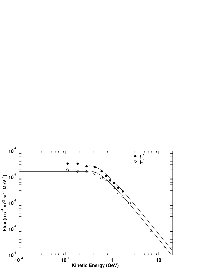
Figure 9: Muon model spectra and reference data of Boezio et al. (2000).

for 10–300 MeV. We could not find data for the upward spectrum and assumed the same function for simplicity. Data of Boezio et al. (2000) were obtained at geomagnetic polar region, whereas GLAST Balloon Experiment was conducted at $R_{\rm cut}\sim 4.5$ GV. They also measured muon spectra at $R_{\rm cut}\sim 4.5$ GV in energy above 2 GeV (Boezio et al., 2003) and obtained a consistent spectrum. A recent measurement by Abe et al. (2003) at $R_{\rm cut}\sim 4.5~{}{\rm GeV}$ also gave a consistent spectrum for energies above 0.5 GeV. We therefore used the model functions above (equation 25 and 26) for the GLAST Balloon Experiment. The ratio of $\mu^{+}$ to $\mu^{-}$, defined as $\frac{\mu^{+}}{\mu^{-}}$, is found to be 1.6 in the data of Boezio et al. (1999b): so we modeled the $\mu^{+}$ spectrum with the same spectral shape but 1.6 times higher normalization. As shown by Boezio et al. (1999b) and Abe et al. (2003), the downward $\mu^{\pm}$ flux is proportional to the atmospheric depth. We therefore assumed the same angular dependence as that of proton secondaries. Our model functions and reference data are given in Figure 9. Note that we do not expect muons in satellite orbit: even for 10 GeV muons the life time is $180~{}\mu s$ in the laboratory frame and they can travel only 50 km.

4 GLAST Balloon Flight

After the integration and test at Stanford Linear Accelerator Center and Goddard Space Flight Center, the instrument was shipped to the National Scientific Balloon Facility (NSBF) in Palestine, Texas. On August 4, 2001, the BFEM was successfully launched. The balloon carried the instrument to an altitude of 38 km in about two hours, and achieved about three hours of level flight until the balloon reached the limit of telemetry from the NSBF. The atmospheric depth at the float altitude was about ${\rm 3.8\ g\ cm^{-2}}$. Due to a small leak of the pressure vessel, the internal pressure went down to 0.14 atmosphere and we failed to record all the data to hard disk. However, a sample of triggered data was continuously obtained via telemetry with about 12 Hz out of a total trigger rate of 500 Hz. More than $10^{5}$ events were recorded during the level flight and showed that all detectors and DAQ system kept working in a space-like high-counting environment. The data obtained allow us to study the cosmic-ray background environment. More details of the preparation and the flight of the BFEM were described in Thompson et al. (2002). In the next section, we compare the simulation prediction with the observed data.

5 Comparison of Data and Simulation

After the flight we found two issues to be taken into account in data analysis. First, three layers out of 26, i.e., 7th layer, 15th layer and 16th layer, were found not to participate in the trigger, although hits in these layers were recorded normally when the trigger condition was satisfied. We took this effect into account in the Geant4 simulation. Fortunately, three or more consecutive pairs of x and y layer (which is the minimum to cause a trigger) worked in the lower part of the TKR (1st to 6th layer), in the middle part of the TKR (9th to 14th layer), and in the upper part of the TKR (17th to 26th layer), and the loss of trigger efficiency due to this failure was only $\sim$ 30%. The second issue was related to the event sampling in telemetry. The sampling unintentionally had a bias toward events with smaller size (primarily number of hits in the TKR) in some data packets. To select unbiased events we required that the packet contain exactly 10 events; a detailed study showed such packets to have an unbiased sample within 10%. This selection reduces the number of events, but we still have 36k events to be used for data analysis.

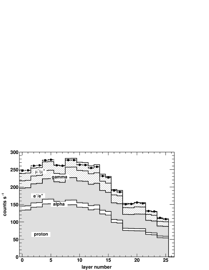
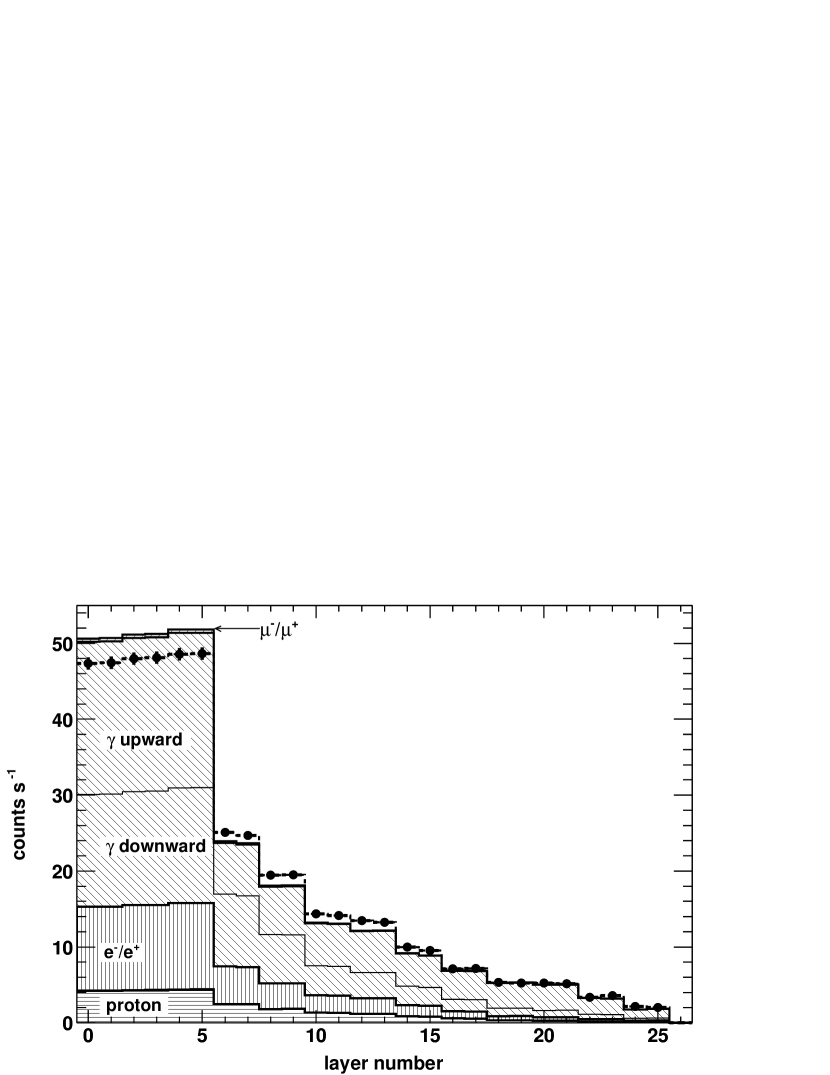
Figure 10: Count rate of each layer for charged (top panel) and neutral (bottom panel) events. Data-points are shown by circles and simulation prediction by histogram. Contribution of each particle type is also shown. For neutral events, contribution of upward gamma and downward gamma is also presented.

In order to validate the cosmic-ray flux model and the Monte-Carlo simulator described in § 2 and § 3, we compared the simulation prediction with the data. The observed trigger rate was about 500 Hz during the level flight and is in good agreement with the simulation prediction. For further study, we divided events into two classes, “charged events” and “neutral events.” A charged event is one in which any one of 13 ACD tiles shows energy deposition above 0.38 MeV (corresponds to 0.2 of the mean energy deposited in an ACD scintillator by a minimum ionizing particle, a MIP). The rates of charged and neutral events observed were 439 Hz and 58 Hz, respectively, and they are reproduced by the simulation within 5%. The contribution of each particle type to the trigger is summarized in Table 3, implying that about 70% of neutral events are from atmospheric gamma-rays. We also compared the count rate of each TKR layer and summarized the results in Figure 10. There, 26 TKR layers are numbered from 0 to 25 in which the layer with number 0 is the closest to CAL. We see jumps in rate between layers 15 and 16, and layers 17 and 18 in charged events. These jumps correspond to the difference of area covered by SSDs described in § 2 (area of 3/5 are covered by Si in layers 18–25, 4/5 are covered in layers 16 and 17, and fully covered in layers 0–15). In neutral events we can see three big rate changes above layers 5, 7 and 9, corresponding to the thick lead converter. The simulation reproduces not only the trigger rate but also these structures very well, validating our instrument simulator and background flux model. The differences between the observations and model are all less than 10%, with the largest difference seen in lower layers (layers 0–5), where the model overpredicts the rates. In this region with no converter layers, the uncertainties of the low-energy electron, positron and gamma-ray models may affect the results. The difference could also be because of the uncertainty of passive materials under the ACD implemented in the simulation.

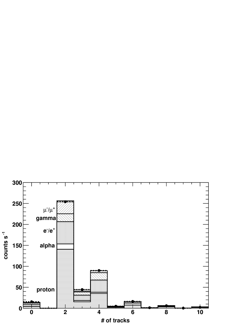
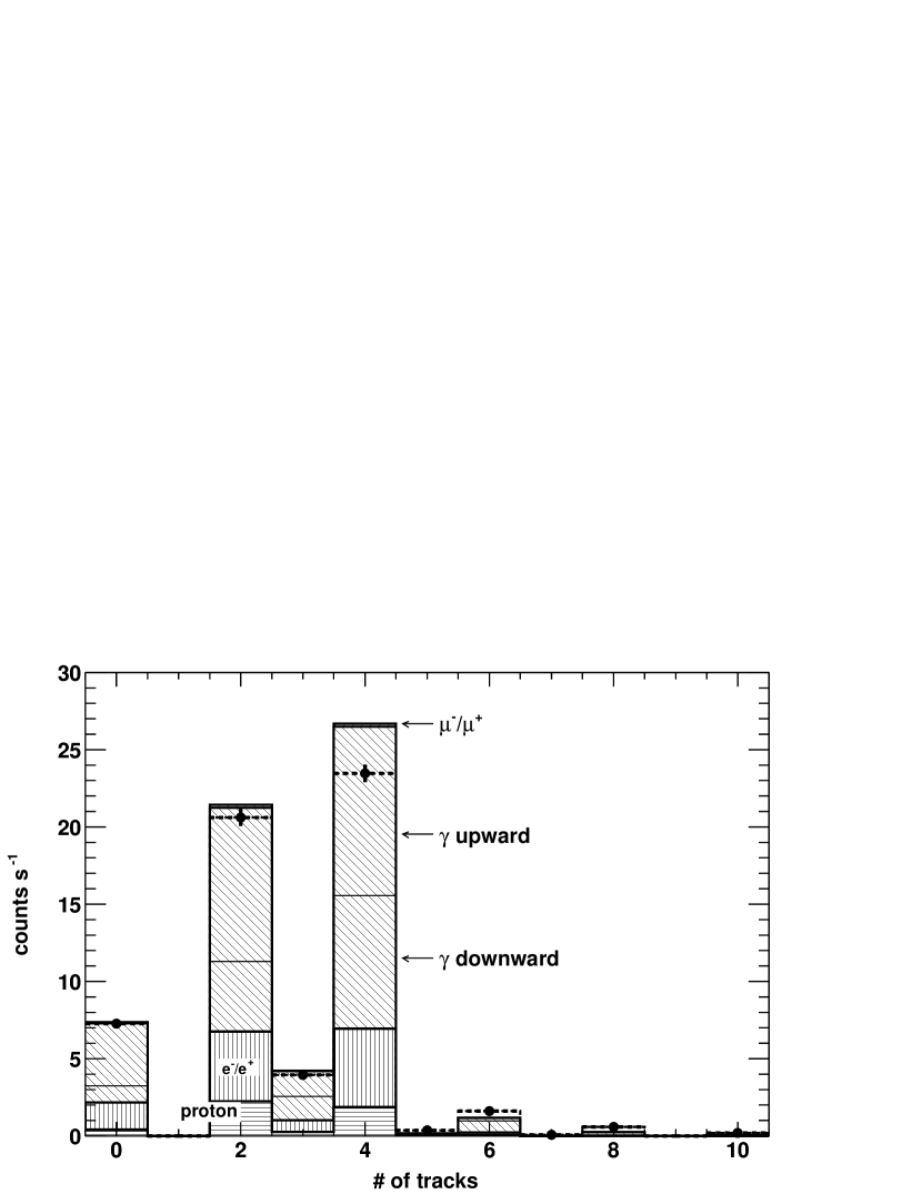
Figure 11: The number of reconstructed tracks of charged (top panel) and neutral (bottom panel) events. Note that the number of tracks is two for single track events (one in x-layer and the other in y-layer) and four for double track events.

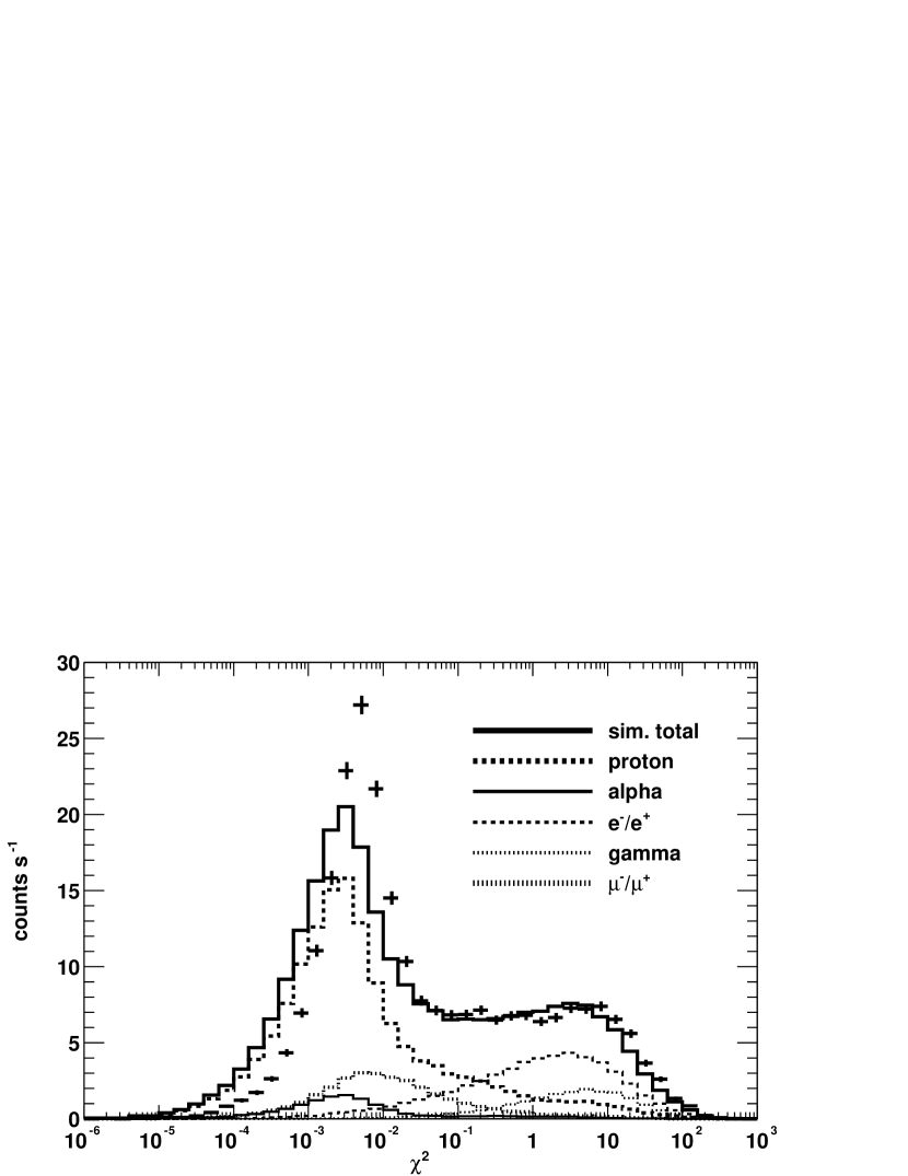
Figure 12: Comparison of the goodness-of-fit (straightness of the track) for single track charged events between data and simulation.

We also applied the event reconstruction program that recognizes the pattern to find the tracks in TKR (Burnett et al., 2002) on both real data and simulation data. The distribution of the number of reconstructed tracks is given in Figure 11, where the number is two for single track events (one in x-layer and the other in y-layer) and is four for double track events. The distribution is well reproduced by simulation for both charged and neutral events. We also selected the single track events out of the charged events and compared the goodness-of-fit ($\chi^{2}$) which evaluates the straightness of the track between data and simulation, as shown in Figure 12. The value of $\chi^{2}$ depends on a particle energy and we set it constant (30 MeV) to obtain a consistent value regardless of whether the particle hits the CAL or not. The two peaks in the figure correspond to tracks with a curved trajectory ($\chi^{2}\geq 0.1$) and those with a straight one ($\chi^{2}\leq 0.1$). The former consists of electrons, positrons, and gamma rays, whereas the latter is composed of protons, alphas and high energy muons. The small difference of the lower peak position between data and simulation could be due to the misalignment of SSDs. Except for this, the data are well reproduced by simulation, providing another evidence that the model flux of each particle type is correct.

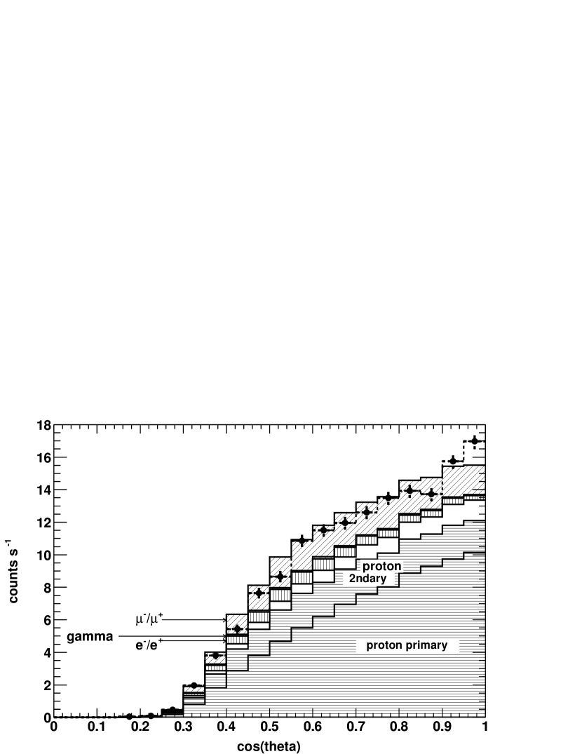
Figure 13: Zenith angle distribution of single and straight track events. Like Figures 10 and 11, data points are given by circles and simulation prediction by histograms. Contribution of each particle type is also presented.

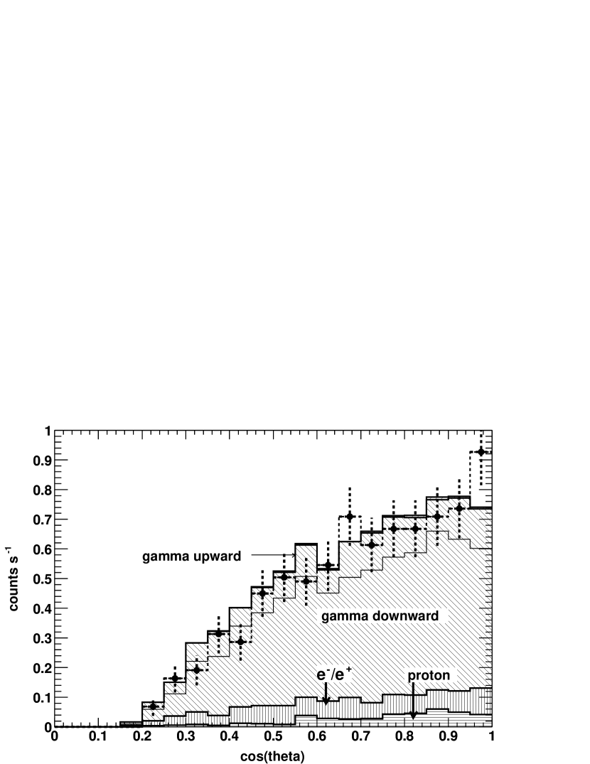
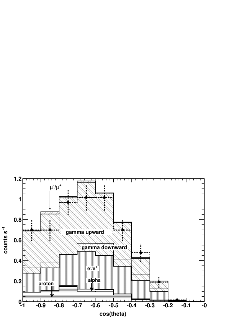
Figure 14: Zenith angle distribution of downward (top panel) and upward (bottom panel) gamma-ray candidates. Contribution of each particle type is also presented. See text for event selection criteria.

Finally we examined the zenith angle distribution of cosmic-ray particles. We first selected single track events with a straight track by requiring $\chi^{2}$ to be less than 0.1, and compared the zenith angle distribution between data and simulation prediction, as shown in Figure 13. In the reconstruction, particles are assumed to go downward, therefore $\cos\theta$ ranges from 1.0 (vertically downward) to 0.0 (horizontal). Our flux model reproduces the data, not only for the vertical direction but also for large zenith angle down to $\cos\theta=0.3$, within 10%. We also applied event selection criteria and studied the gamma-ray zenith-angle distribution. The cuts we used here are not optimized for background reduction, for the number of events is limited. Instead, we implemented a set of loose cuts to filter out charged particles and save a sufficient number of gammas. To select downward gammas, we required events with no hit in the ACD, double tracks in the TKR, and gaps between two tracks increasing as they go downward (downward-opening v-shape trajectory). For upward gammas, we did not require that the event be neutral, since the generated electron/positron pair is expected to hit the ACD. Instead, we required that the two bottommost TKR layers did not detect a hit and the TKR showed double tracks with upward-opening v-shape trajectory. We also set CAL energy threshold at 6 MeV, half of the energy deposition by MIP crossing one CsI log, to eliminate events with interaction in CAL. The results are shown in Figure 14 in which the bisector of two tracks are assumed to be the direction of gamma. Data are well reproduced by simulation down to $\cos\theta=0.3$ for downward and up to $\cos\theta=-0.3$ for upward, validating the spectral and angular distribution models for gammas.

6 Sensitivity of the Model to Assumptions

The background flux model used to compare with the BFEM data involves many parameters, some of which are poorly defined. In the course of this investigation, we tried a number of alternate assumptions in cases where no well-defined observations were available. The extent to which such alternatives affected the agreement with the data provides an indication of how sensitive the model is to such parameters. Below we list some of these possibilities and describe their influence on the comparison.

$\bullet$ Fluxes of secondary proton, electron, and positron were at one time derived directly from the AMS measurements. Models based on balloon measurements increased the trigger rate by about 15% and improved the agreement of charged events.

$\bullet$ The model function of the secondary upward-moving gamma-ray flux were at one time simpler: in 1 MeV to 1 GeV, it was expressed by a single power-law function of index of -1.7, with 1.6 times higher normalization at 1 MeV. The new model increased the neutral event rate by about 15% and improved the match between BFEM data and simulation prediction.

$\bullet$ We once expressed the angular dependence of the secondary charged particles by $1+0.6\sin\theta$, an empirical model given in old rocket measurements (Van Allen & Gangnes, 1950a, b; Singer, 1950). The new model did not alter the trigger rate nor the angular distribution shown by Figure 13 very much. We adopted our model to take into account the fact that proton and muon secondary fluxes are proportional to the atmospheric depth, although the BFEM data alone could not determine which model is better.

$\bullet$ As described in § 3, fluxes of secondary $e^{-}/e^{+}$ and upward gamma are poorly known, although these particles contributes to the trigger significantly. Detailed study showed that the main component of secondary $e^{-}/e^{+}$ which causes the trigger is of energy of about 100 MeV and that of upward gamma is of energy of 10–100 MeV, where the particle fluxes are uncertain by a factor of 2–3. However, if we change the $e^{-}/e^{+}$ flux by 50%, the trigger rate of charged event is changed by $\sim 50~{}{\rm c~{}s^{-1}}$ and disagrees with data. Similar disagreement will arise in neutral event rate by adjusting the flux of upward gamma.

With a substantial number of parameters in this model, we cannot be certain that all of them are simultaneously optimized. What we have found is that specific variations in model parameters tend to affect only one aspect of the comparison between the model and the BFEM observations. The fact that we have obtained reasonable agreement with this range of observables - total rate, rate per layer, charged component, neutral component, straight tracks, curved tracks, and angular distribution - suggests that the model is a good approximation to reality.

7 Summary

We have constructed the GLAST BFEM instrument simulator with a Geant4 toolkit (§ 2) and the background flux models of abundant components (proton, alpha, electron, positron, gamma ray and $\mu^{-}/\mu^{+}$) based on previous measurements and theoretical predictions (§ 3). The simulation successfully reproduces the observed data within 10%, indicating that the flux model is a good representation of the cosmic-ray background at balloon altitude at Palestine, Texas. Models for the entire low-Earth orbit are also given in § 3, where the effect of cutoff rigidity and solar modulation potential are parameterized. They are being used for the simulation of GLAST LAT in orbit and the study of the background rejection.

The authors would like to thank assistance given by M. Sjögren, K. Hirano and H. Mizushima in various phases of this work. They are also grateful to A. Tylka, R. Battiston, Y. Komori, A. Yamamoto and T. Yoshida for helpful discussions about the cosmic-ray background flux. They would also like to thank E. do Couto e Silva, H. Tajima, T. Kotani, R. C. Hartman, L. Rochester, T. Burnett, R. Dubois, J. Wallace and GLAST BFEM team and GLAST LAT collaboration for their support and discussions. They also would like to thank the staff of National Scientific Balloon Facility for their excellent support of launch, flight and recovery.

Table 1: Model parameters for proton secondary flux at satellite altitude, based on AMS data.

region	direction	model	parameters
$0.0\leq\theta_{\rm M}\leq 0.2$	down/upward	cutoff PL	0.136/0.123/0.155/0.51
$0.2\leq\theta_{\rm M}\leq 0.3$	down/upward	broken PL	0.1/0.87/600/2.53
$0.3\leq\theta_{\rm M}\leq 0.4$	down/upward	broken PL	0.1/1.09/600/2.40
$0.4\leq\theta_{\rm M}\leq 0.5$	down/upward	broken PL	0.1/1.19/600/2.54
$0.5\leq\theta_{\rm M}\leq 0.6$	down/upward	broken PL	0.1/1.18/400/2.31
$0.6\leq\theta_{\rm M}\leq 0.7$	downward	broken PL	0.13/1.1/300/2.25
	upward		0.13/1.1/300/2.95
$0.7\leq\theta_{\rm M}\leq 0.8$	downward	broken PL	0.2/1.5/400/1.85
	upward		0.2/1.5/400/4.16
$0.8\leq\theta_{\rm M}\leq 0.9$	downward	cutoff PL	0.23/0.017/1.83/0.177
	upward	broken PL	0.23/1.53/400/4.68
$0.9\leq\theta_{\rm M}\leq 1.0$	downward	cutoff PL	0.44/0.037/1.98/0.21
	upward	broken PL	0.44/2.25/400/3.09

Table 2: The same as Table 1, but for $e^{-}/e^{+}$ instead of proton.

region	$\frac{e^{+}}{e^{-}}$ ratio	model	parameters for $e^{-}$ spectrum
$0.0\leq\theta_{\rm M}\leq 0.3$	3.33	broken PL	0.3/2.2/3/4.0
$0.3\leq\theta_{\rm M}\leq 0.6$	1.66	PL	0.3/2.7
$0.6\leq\theta_{\rm M}\leq 0.8$	1.0	PL+hump	0.3/3.3/$2.0\times 10^{-4}$/1.5/2.3
$0.8\leq\theta_{\rm M}\leq 0.9$	1.0	PL+hump	0.3/3.5/$1.6\times 10^{-3}$/2.0/1.6
$0.9\leq\theta_{\rm M}\leq 1.0$	1.0	PL	0.3/2.5

Table 3: Contribution of each particle type to the trigger rate, in unit of Hz.

particle type	proton	alpha	$e^{-}$/$e^{+}$	$\gamma$ 2ndary	$\gamma$ 2ndary	$\mu^{\pm}$	total	data
				downward	upward
charged events	216	19	110	12	42	39	438	439
neutral events	4.8	0.1	12.3	16.8	26.8	0.5	61.3	58.2

References

- Abe et al. (2003) Abe, K., et al. 2003, Physics Letter B, 564, 8
- Agostinelli et al. (2003) Agostinelli, S., et al., 2003, Nuclear Instruments and Methods A, 506, 250
- Alcaraz et al. (2000a) Alcaraz, J., et al. 2000a, Physics Letter B, 472, 215
- Alcaraz et al. (2000b) Alcaraz, J., et al. 2000b, Physics Letter B, 484, 10
- Alcaraz et al. (2000c) Alcaraz, J., et al. 2000c, Physics Letter B, 490, 27
- Alcaraz et al. (2000d) Alcaraz, J., et al. 2000d, Physics Letter B, 494, 193
- Barwick et al. (1998) Barwick, S. W., et al. 1998, Journal of Geophysical Research, 103, 4817
- Boezio et al. (1999a) Boezio, M., et al. 1999a, ApJ, 518, 457
- Boezio et al. (1999b) Boezio, M., et al. 1999b, Physical Review Letters, 82, 4757
- Boezio et al. (2000) Boezio, M., et al. 2000, Physical Review D, 62, 032007
- Boezio et al. (2003) Boezio, M., et al. 2003, Physical Review D, 67, 072003
- Burnett et al. (2002) Burnett, T. H., et al. 2002, IEEE Transactions on Nuclear Science, 49, 1904
- Couto e Silva et al. (2001) Couto e Silva, E. do, et al. 2001, Nuclear Instruments and Methods A, 474, 19
- Daniel & Stephens (1974) Daniel, R. R., & Stephens, S. A. 1974, Rev. Geophys. Space Phys. 12, 233
- DuVernois et al. (2001) DuVernois M. A., et al., 2001, Proceeding of 27th International Cosmic Ray Conference, 3, 61
- Gehrels & Michelson (1999) Gehrels, N., & Michelson, P. 1999, Astroparticle Physics, 11, 277
- Gleeson & Axford (1968) Gleeson, L. J., & Axford, W. I. 1968, ApJ, 154, 1011
- Golden et al. (1994) Golden, R. L., et al. 1994, ApJ, 436, 769
- Imhof, Nakano, & Reagan (1976) Imhof, W. L., Nakano, G. H., & Reagan, J. B. 1976, Journal of Geophysical Research, 81, 2835
- Israel (1969) Israel, M. H. 1969, Journal of Geophysical Research, 74, 4701
- Kur’yan et al. (1979) Kur’yan, Y. A., Mazets, Y. P., Proskura, M. P., & Sokolov, I. A. 1979, Geomagnetism and Aeronomy, 19, 6
- Longair (1992) Longair, M. S. 1992, High Energy Astrophysics, vol. 1 (2nd edition; Cambridge: Cambridge University Press)
- Menn et al. (2000) Menn, W., et al., 2000, ApJ 533, 281
- Moskalenko & Strong (1998) Moskalenko, I. V., & Strong, A. W. 1998, ApJ, 493, 694
- Pennypacker et al. (1973) Pennypacker, C. R., Smoot, G. F., Buffington, A., Muller, R. A., & Smith, L. T. 1973, Journal of Geophysical Research, 78, 1515
- Ryan et al. (1979) Ryan, J. M., Jennings, M. C., Radwin, M. D., Zych, A. D., & White, R. S. 1979, Journal of Geophysical Research, 84, 5279
- Sanuki et al. (2000) Sanuki, T., et al., 2000, ApJ, 545, 1135
- Seo et al. (1991) Seo, E. S., Ormes, J. F., Streitmatter, R. E., Stochaj, S. J., Jones, W. V., Stephens, S. A., & Bowen, T. 1991, ApJ, 378, 763
- Shönfelder et al. (1977) Shönfelder, V., Graser, U., & Daugherty, J. 1977, ApJ, 217, 306
- Shönfelder et al. (1980) Shönfelder, V., Graml, F., & Penningsfeld, F. -P. 1980, ApJ, 240, 350
- Singer (1950) Singer, S. F. 1950, Physical Review Letters, 77, 729
- Sreekumar et al. (1998) Sreekumar, P., et al., 1998, ApJ, 494, 523
- Thompson (1974) Thompson, D. J. 1974, Journal of Geophysical Research, 79, 1309
- Thompson, Simpson & Özel (1981) Thompson, D. J., Simpson, G. A., & Özel, M. E. 1981, Journal of Geophysical Research, 86, 1265
- Thompson et al. (2002) Thompson, D. J., et al., 2002, IEEE Transactions on Nuclear Science, 49, 1898
- Van Allen & Gangnes (1950a) Van Allen, J. A., & Gangnes, A. V. 1950a, Physical Review, 78, 50
- Van Allen & Gangnes (1950b) Van Allen, J. A., & Gangnes, A. V. 1950b, Physical Review, 79, 51
- Verma (1967) Verma, S. D. 1967, Journal of Geophysical Research, 72, 915
- Webber (1983) Webber, W. R. 1983, in Composition and Origin of Cosmic Rays, ed. M. M. Shapiro, (Dordrecht: D. Reidel Publishing Co.), 83
- Zombeck (1990) Zombeck M. V. 1990, Handbook of space astronomy and astrophysics (2nd edition; Cambridge: Cambridge University Press)