Inter–cluster filaments in a $\Lambda$CDM Universe

Abstract

The large–scale structure (LSS) in the Universe comprises a complicated filamentary network of matter. We study this network using a high–resolution simulation of structure formation in a $\Lambda$ Cold Dark Matter cosmology. We investigate the distribution of matter between neighbouring large haloes whose masses are comparable to massive clusters of galaxies. We identify a total of 228 filaments between neighbouring clusters. Roughly half of the filaments are either warped or lie off the cluster–cluster axis. We find that straight filaments, on the average, are shorter than warped ones. Close cluster pairs with separation of 5 $h^{-1}$ Mpc or less are always connected by a filament. At separations between 15 $h^{-1}$ Mpc and 20 $h^{-1}$ Mpc about a third of cluster pairs are connected by a filament. On average, more massive clusters are connected to more filaments than less massive ones. This finding indicates that the most massive clusters form at the intersections of the filamentary backbone of LSS. For straight filaments, we compute mass profiles. Radial profiles show a fairly well–defined radius, $r_{s}$, beyond which the profiles follow an $r^{-2}$ power law fairly closely. For the majority of filaments, $r_{s}$ lies between 1.5 $h^{-1}$ Mpc and 2.0 $h^{-1}$ Mpc. The enclosed overdensity inside $r_{s}$ varies from a few times up to 25 times the mean density, independent of the length of the filament. Along the filaments’ axes, material is not distributed uniformly. Towards the clusters, the density rises, indicating the presence of the cluster infall regions. Filaments have been suggested to cause possible alignments between neighbouring clusters. Looking at the nearest neighbour for each cluster, we find that, up to a separation of about 15 $h^{-1}$ Mpc, there is a filament present that could account for alignment. In addition, we also find some sheet–like connections between clusters. In roughly a fifth of all cluster–cluster connections where we could not identify a filament or sheet, projection effects lead to filamentary structures in the projected mass distribution.

1 Introduction

Large galaxy redshift surveys such as the Sloan Digital Sky Survey (York et al. 2000) and the 2dFGRS (Colless et al. 2001) and N–body simulations of cosmic structure formation (for example Jenkins (1998), Wambsganss et al. (2004)) show a complicated network of matter. In redshift surveys, the galaxies line up preferentially around roundish, almost empty regions – so–called voids. Clusters of galaxies have very prominent positions in the network: They lie at the intersections of filaments. In N–body simulations, this trend is even more pronounced. The network of haloes is clearly followed by the more diffusely distributed component of the dark matter that, at $z=0$, has not collapsed into haloes.

Describing this network is no easy task. There are a wide variety of statistical and topological tools to compare observations and theoretical models. Amongst these are the two–point (and higher–order) correlation function(s) (e.g. Peebles, 1980; Peebles & Groth, 1975), minimal spanning trees (see e.g. Barrow et al., 1985; Krzewina & Saslaw, 1996; Bhavsar & Splinter, 1996), the genus statistics (Gott et al., 1986), Minkowski functionals (that include the genus; Mecke et al., 1994), shape statistics (see e.g. Babul & Starkman, 1992; Luo & Vishniac, 1995; Luo et al., 1996), and shapefinder statistics derived from Minkowski functionals (Sahni et al., 1998; Sheth et al., 2003; Shandarin et al., 2004). These tools have all been applied to galaxy catalogues and N–body simulations and have been very useful in comparing observations and theory.

These tools have been somewhat less helpful in describing the pattern of large–scale structure as far as filaments and sheets/walls are concerned. Minkowski functionals and especially their shapefinder cousins have been used to try to measure how thick or long filaments are. By construction, for simple toy models like ideal filaments (cylinders) or sheets (planes), shape statistics give very simple answers. Because of the complexity of the network of matter in surveys or simulations the answers for these cases are usually more difficult to interpret than in the toy model simulations. Recently, Bharadwaj et al. (2004) investigated filaments in the Las Campanas Redshift Survey using shapefinders. Adding statistical tools to their machinery, they looked at the maximum length scale at which filaments in that survey are statistically significant. They found that scale to be 50 $h^{-1}$ Mpc to 70 $h^{-1}$ Mpc. Another very promising approach has been suggested by Stoica et al. (2004). They introduce another method to actually detect filaments. Their method is based on an algorithm that has been successfully used to detect road networks, and they showed that it works very well for 2D mock data sets.

In this work, we will restrict our focus mainly to filaments. In slices through N–body simulations (see for example Jenkins, 1998) filaments appear to be very common. There is some variety in their sizes and appearance. The most massive haloes are usually connected by very prominent filaments (see Figure 1). However, some of the filaments could be sheets and only appear to be filamentary due to projection effects. Less dense and less massive filaments can be found in less dense regions – those filaments resemble fine perl necklaces. In an earlier work (Colberg et al., 1999), we showed that the formation of clusters is intimately linked with the cosmic neighbourhood. Infall of matter into the region where a cluster is forming happens from a few preferred directions. These agree with the locations of filaments at $z=0$.

Here, we will investigate the properties of filaments in more detail. In particular, we will address the following set of questions: On average, how many filaments intersect at the location of a cluster? Does the number of filaments depend on the mass of the cluster? What is the typical density of a filament? How long are these filaments typically? For a pair of clusters at some separation what is the likelihood of finding a filament between them?

This paper is organized as follows: After a brief discussion of earlier theoretical work (2), in Section 3, we discuss the status of observations to locate filaments. Afterwards (Section 4), we briefly describe the simulation that we use (Section 4.1) and then the procedure (Section 4.3) to look at cluster–cluster connections. We present a classification of those connections in Section 4.4. Section 4.5 describes properties of filaments and of clusters connected to such filaments. In Section 4.5 we also discuss what our results might mean for alignments of clusters. We conclude the paper with a summary (Section 5).

2 Theoretical work

Anisotropic collapse of matter in gravitational instability scenarios has been known to lead to the formation of sheets and filaments since the seminal work by Zel’dovich (1970) (also see Shandarin & Zeldovich, 1989). Icke (1973) looked at the effect using homogeneous ellipsoidal models (also see the work by White & Silk, 1979; Eisenstein & Loeb, 1995). Bond et al. (1996) then emphasized the role of tidal fields and of anisotropic collapse in the formation of LSS. They connected tidal shear directly to the locations of filamentary structures and of peaks.

That same year, van de Weygaert & Bertschinger (1996) investigated the typical morphology of a configuration of two clusters with material in between to find that the primordial shear constraint naturally evolves into a configuration of two clusters that are connected by a filament. Van de Weygaert (2002) contains a very detailed summary of these theoretical efforts.

There have also been theoretical studies of gas in filaments, the so–called warm–hot intergalactic medium (WHIM), using simulations. The WHIM contains a significant fraction of all baryons in the present-day universe (about 30% to 40%), which makes observing filaments through the signature of their baryons quite interesting. For the most recent studies see Davé et al. (2001), Kravtsov et al. (2002), and Furlanetto et al. (2003) and references therein.

3 Observational status

The questions we posed in the introduction are of particular interest given observational efforts to find filaments by looking at the space in the vicinities of clusters. Gray et al. (2002) and Dietrich et al. (2004) looked at cluster pairs A901/A902 and A222/A223, respectively. Using weak lensing they both conclude that the two clusters in their respective surveys are connected by a filament. Pimbblet & Drinkwater (2004) used clusters A1079 and A1084 in a pilot study to look for filaments, reporting a “filament detection at a 7.5$\sigma$ level.” Tittley & Henriksen (2001) used x–ray data to detect a filament between clusters A3391 and A3395.

The most relevant detection of a filament that was not found by looking at clusters directly is by Scharf et al. (2000). They found a “5$\sigma$ significance half–degree filamentary structure”, present both in x–ray and optical data. At a likely redshift of around $\gtrsim$ $z=0.3$, Scharf et al. (2000) give the length of the structure as $\gtrsim$ 12 $h_{50}^{-1}$ Mpc.

Superclusters are very likely locations of filaments or even sheets. For example, Connolly et al. (1996) found a large structure at a redshift of $z=0.54$ with an overdensity (in galaxies) of about four that includes three X–ray clusters. The galaxies in this sample form “a linear structure passing from the Southwest of the survey field through to the Northeast.” More recently, Bregman et al. (2004) looked at filaments in superclusters through UV absorption line properties of three AGNs projected behind possible filaments in superclusters. They conclude that their results are consistent with the presence of filaments.

At somewhat larger redshifts, Gal & Lubin (2004) investigated two clusters at redshifts of $a\approx\,0.9$ which appear to be connected by a large structure. Ebeling et al. (2004) detected a structure of galaxies extending out from the cluster MACS J0717.5+3745, that is located at a redshift of $z=0.55$, with a length of 4 $h_{70}^{-1}$ Mpc.

Kaastra et al. (2003) observed a sample of 14 clusters, looking for soft X–ray excess emission. For five of their clusters they find “a significant soft excess,” which they attribute to emission from intercluster filaments of the WHIM in the vicinity of these clusters.

All these works are very exciting and indicate that there will be many more such projects in the very near future. We thus feel that answering the questions about what one can expect to find is all the more relevant.

Figure 1: A slice of thickness $10\,h^{-1}$ Mpc through the GIF simulation. The dark matter was smoothed adaptively, and the resulting density field is shown using a logarithmic colour scale. We have marked the location of the filament that is shown in Figure 3 with a box. In order to emphazise the rôle of the clusters we have included the clusters inside the box. The width of the box – its dimension perpendicular to the cluster–cluster axis – is $15\,h^{-1}$ Mpc, which is the actual diameter of the cylinders used to cut out filaments. – Download from http://lahmu.phyast.pitt.edu/$\sim$colberg/GIF_10_42_z.jpg

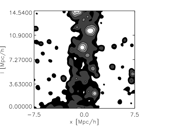
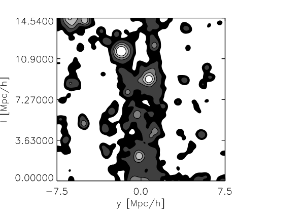
Figure 2: Two orthogonal projections of the dark matter between two of the clusters in the GIF simulation. The plots show the projected overdensities, smoothed with a Gaussian of radius 0.5 $h^{-1}$ Mpc. The contour levels show overdensities ranging from 0.0 (mean density, black) to 19.0 (white). The $y$–axis cuts through both cluster centers. The region shown here excludes the clusters themselves. Matter follows a filamentary pattern.

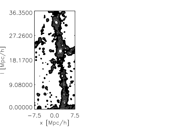
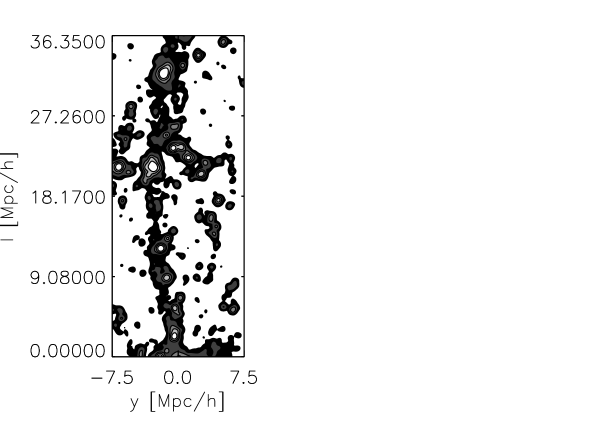
Figure 3: Same as Figure 2 for a moderately warped filament. Please note that this cluster–cluster connection is longer than the one shown in Figure 2.

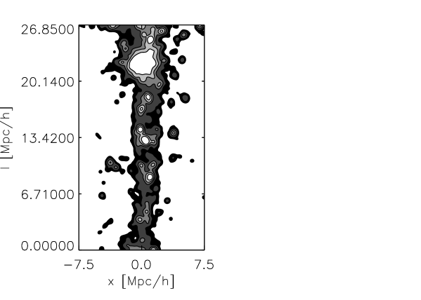
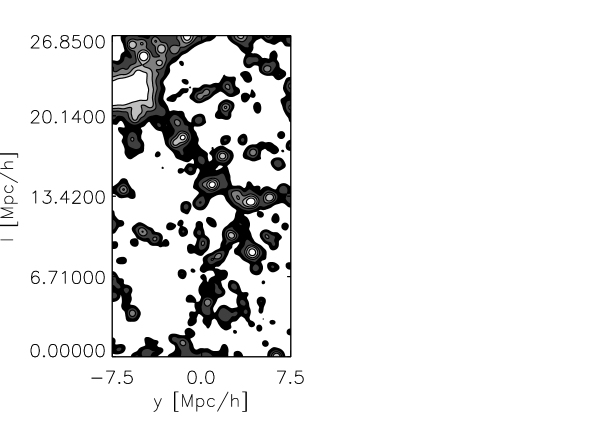
Figure 4: Same as Figure 2 – again with a longer connection – for matter lying in a sheet. Note the presence of another cluster inside the sheet but outside of the 5 $h^{-1}$ Mpc exclusion zone (see discussion).

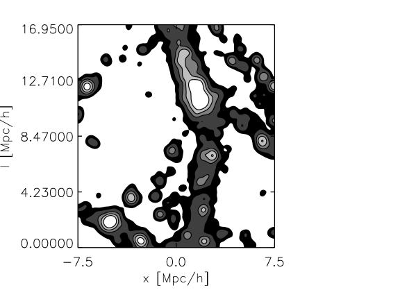
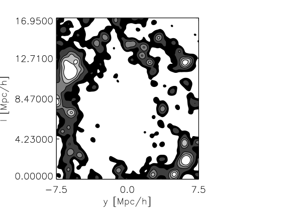
Figure 5: Same as Figure 2 – again with different length scale – for matter that appears to be filamentary from one direction (left panel). Viewed from another direction – on the right–hand side from a direction perpendicular to the one on the left–hand side there is no visible filament. The filament on the left–hand side is merely caused by a projection effect.

4 The inter–cluster network of matter

4.1 The simulation

For this work, we use the $\Lambda$CDM simulation introduced in Kauffmann et al. (1999). The simulation parameters correspond very closely to what has recently become the standard cosmology with 30% of the critical density contributed by Cold Dark Matter and the remaining 70% by a cosmological constant (or “Dark Energy”). A Hubble constant of $h=0.7$ is used and the model is cluster normalized to $\sigma_{8}=0.9$. With $256^{3}$ particles in a box of size (141.3 $h^{-1}$ Mpc)³ the simulation volume is large enough to study large–scale structure at high resolution.

4.2 Visual impression

Figure 1 shows a slice of thickness $10\,h^{-1}$ Mpc through the simulation volume. The dark matter distribution was smoothed adaptively, and the resulting density field is shown using a logarithmic colour scale. The slice shows the network of matter, which is quite familiar from simulation work and from galaxy redshift surveys.

We have marked the location of the filament that is shown in Figure 3 with a box. In order to emphazise the rôle of the clusters we have included the clusters inside the box (Figure 3 shows just the material inside the filaments, excluding the clusters). The width of the box – its dimension perpendicular to the cluster–cluster axis – is $15\,h^{-1}$ Mpc, which is the actual diameter of the cylinders used to cut out filaments. Figure 1 gives a good impression of the extent of the longer filaments in our sample.

4.3 The procedure

First, we extract clusters from the halo catalogue that we downloaded from the website of the Max–Planck–Institut für Astrophysik. We consider all haloes more massive than 10¹⁴ M_⊙. This provides a sample of 170 clusters whose number density is roughly comparable to that of R=0 Abell clusters (Postman et al., 1992).

Since we are interested in the inter–cluster network of matter, we examine the twelve nearest neighbours of each cluster. For each pair of clusters we extract the dark matter between them as follows. The cluster centers define an axis. We extract all dark matter particles in a cylinder of radius 7.5 $h^{-1}$ Mpc around the axis. Furthermore, we only work with those particles that, when projected onto the axis, lie outside both clusters’ $r_{200}$. That way, we do not extract matter that belongs to either cluster. However, matter that lies in the cluster–infall regions is included in the samples. The value of 7.5 $h^{-1}$ Mpc is empirical (as is the number of twelve cluster neighbours). We found that going further out does not add any extra information whereas using smaller radii sometimes tended to cut warped filaments in half.

There is one final requirement for how neighbouring clusters were picked. Because we are interested in the inter–cluster network of matter we want to avoid finding one cluster lying directly between two other clusters. We thus do not allow another cluster to lie inside the innermost 5 $h^{-1}$ Mpc from the cluster–cluster axis. As before, this value is empirical.

We want to emphasize that most certainly there will be many configurations where a number of clusters are lined up on a long filament. We exclude these cases for the simple and only reason that we want to study the distribution of matter between two neighbouring clusters. In a follow–up study, we will come back to looking at the alignment of clusters on larger scales.

4.4 Classifying inter–cluster connections

Conventional wisdom says that if one picks two neighbouring clusters, they are connected by a filament, they lie in a sheet, or there is a void between them. In reality, the number of possibilities is slightly more complicated. The following list of the configuration of matter between neighbouring clusters is based on the visual inspection of each of the cluster–cluster connections. We tried to automate the process by using density measures but there are too many cases with deviations from the simple configurations mentioned above.

Filaments: 19% of the 1207 cluster–cluster connections contain a filament. We found three different possible configurations:

straight: 38% of all filaments are straight and on center with respect to the cluster–cluster axis.That is, the clusters lie on the axis of the filament. See Figure 2.

off center: Another 9% of all filaments are also fairly straight filaments but their central axes do not align with the axis that connects the cluster centers.

warped/irregular: 53% of all filaments are not straight but are either warped or consist of multiple parts. Warped filaments sometimes indicate the presence of another cluster that lies just outside the 5 $h^{-1}$ Mpc exclusion zone. When we looked at the matter distribution of warped filaments going beyond the cylinder used for the analysis we found many cases where nearby mass concentrations must have tidally interacted with the filaments. See Figure 3.

Sheets: In about 2% of all cases, we found a sheet–like configuration between cluster pairs. Sheets display a narrow extent when viewed edge on and a broad uniform distribution of matter otherwise. See Figure 4.

The Rest: The remaining 79% of cluster–cluster pairs do not fall into the aforementioned categories. However, there are some interesting cases left. In 3% of all cluster pairs we found a large amount of matter between them that does not look either filamentary or sheet–like. Instead, viewed from any angle matter fills the space between the clusters almost uniformly. In 19% of all cases that were not classified as a filament, sheet or crowded field projection effects lead to the appearance of filaments. When viewed from one angle there seems to be a filament, whereas viewed from another angle there is none (see Figure 5). There is the possibility of a sheet being mis–classified as a projection effect or vice versa – especially since the classification is done by eye. However, since we focus our work on studying filaments this uncertainty does not affect the bulk of our results. Projection effects and, to a lesser extent, sheets have to be kept in mind when looking at actual measurements of the distribution of matter between clusters by means of gravitational lensing as results from these very different configurations will appear the same.

4.5 Properties of inter–cluster filaments

Our sample of straight and warped filaments is large enough to allow more detailed studies of their properties. It is important to bear in mind the restrictions imposed on the analysis by how we selected the filaments. By filament we mean a filament that connects two clusters. The filament could be a segment of a larger filament that connects more than two clusters. We do not attempt to study large filaments in more detail here. Whenever we are talking about filaments in the following we mean filaments between pairs of clusters.

Figure 6: Fractional abundance of filaments: The plot shows the fractions of cluster–cluster connections that contain a filament – straight or warped – as a function of length of those connections. Close cluster pairs are always connected by a filament.

Figure 7: Length distributions of filaments: The plot shows the fraction of filaments (solid line) and warped filaments (dotted line) that have a length $l$. Warped filaments tend to be longer than straight filaments.

Figure 8: Enclosed overdensity profile of a straight filament. The bold vertical line shows the radius at which the profile starts to follow an $r^{-2}$ power law.

Figure 9: Distribution of scale radii $r_{s}$ of straight filaments.

Figure 10: For straight filaments, this plot shows the enclosed overdensity at scale radius $r_{s}$ versus the length of the filament.

Figure 11: Longitudinal density profile of straight filaments, averaged over straight filaments that are longer than 5 $h^{-1}$ Mpc. Shown is the enclosed overdensity as a function of the positions along the cluster–cluster axis for all material that is contained within 2 $h^{-1}$ Mpc from the axis.

4.5.1 General properties of cluster–cluster filaments

The first questions to ask about filaments are how long and how common they are. As we noted before, we looked at 1207 regions between neighbouring clusters of which 19% contained a filament. We selected the pairs of clusters by picking the twelve nearest neighbours of a given cluster. Given the fact that in the large–scale structure matter surrounds large voids, the relatively small number of filaments does not come as a surprise. If we had required that the cluster–cluster connections did not intersect voids we would have ended up with a larger overall percentage of filaments.

Nevertheless, it is interesting to look at the abundance of filaments for a given separation between two clusters. Figure 6 shows the fractions of cluster–cluster connections that contain a filament – straight or warped – as a function of the length of those connections. Very close cluster pairs are always connected by a filament, and about a third of all cluster pairs whose separation is between 15 $h^{-1}$ Mpc and 20 $h^{-1}$ Mpc are connected by a filament.

The fact that very close pairs of clusters – with separations of up to 5 $h^{-1}$ Mpc – are always connected by a filament can be explained by the presence of cluster infall regions. As discussed in, e.g., Diaferio & Geller 1997, the infall region of a cluster extends out to about three times its virial radius. What this means is that two very close clusters do not constitute two strictly separated systems as their infall regions overlap, and if they are gravitationally bound, the two clusters may eventually merge. Indeed, close cluster pairs show the presence of a filament between them (Dietrich et al., 2004).

Figure 7 shows the length fractions of straight and warped filaments (strictly speaking, for warped filaments the length $l$ is not the length of the filament but the length of the cluster–cluster connection). On the average, straight filaments are shorter than warped filaments. Two thirds of all straight filaments are in the 5 $h^{-1}$ Mpc to 15 $h^{-1}$ Mpc range whereas warped filaments have a much broader distribution that extends out to fairly large separations. Clearly, tidal fields must play a role here. In fact the visual impression is that many warped filaments are bent towards another mass concentration.

The most interesting properties of filaments are the amount of matter and its spatial distribution inside the filament. We investigated these quantities for our sample of straight filaments as follows. As noted above, all filaments were identified visually. In almost all cases the axes of the straight filaments deviate somewhat from the cluster–cluster axis. Therefore, for each filament we compute the actual axis by projecting all particles onto the plane perpendicular to the cluster–cluster axis and then computing the center of mass of the particles in that plane. The resulting center of mass is located where the filament’s axis intersects with the plane. We then use this axis to compute the enclosed (radial) mass profile by averaging over all angles.

The resulting profiles show a very interesting behaviour. There is a fairly large variation in the profiles close to the filaments’ axes. However, for each filament we find that at some radius, $r_{s}$, the profile starts following an $r^{-2}$ power law closely. For each filament, we determine that radius, $r_{s}$, by finding the part of the profile that can be fit by an $r^{-2}$ power law. As an example, Figure 8 shows the radial overdensity profile of one filament. The bold vertical line marks $r_{s}$. The existence of the radius $r_{s}$ indicates that filaments have a well–defined edge. With the mass of a filament $M_{fil}(>r_{s})\approx const.$ but the volume growing as $r^{2}$ (the length $l=const.$) the enclosed overdensity of the filament $\delta(<r)\propto r^{-2}$.

In Figure 9 we plot the distribution of the radii $r_{s}$. The majority of filaments posess radii $r_{s}$ between 1.0 $h^{-1}$ Mpc and 2.0 $h^{-1}$ Mpc but there are also narrower and wider filaments.

Given that filaments have well–defined edges how much matter is contained in a filament and does the amount of matter depend on the length of the filament? Figure 10 shows for each filament the enclosed overdensity at $r_{s}$ versus the length of the filament. There is no obvious trend with length, but there is a fairly large scatter in the enclosed matter. There are even a few cases where the enclosed overdensity exceeds 30. We visually inspected these cases and found that for every such case there is at least one very large halo present that lies on the filament’s axis and whose mass is below the cluster threshold mass used for this work.

The radial density profiles of filaments have quite interesting repercussions for observational efforts to find filaments. Given that filaments have well–defined edges with no dependences on length and with fairly large possible masses finding them observationally could be easier than previously thought. Either surveys using gravitational lensing or direct observations of galaxies in the vicinity of galaxy clusters (Ebeling et al., 2004) appear to be very promising in this light.

Figure 11 shows the averaged longitudinal overdensity profile of straight filaments. For these, we normalized the length of all filaments to unity and excluded cluster pairs with separations less than 5 $h^{-1}$ Mpc. We then computed the enclosed density of all material that is contained within 2 $h^{-1}$ Mpc from the filament’s axis as a function of the position along the axis. The overdensity rises towards the clusters and is constant at a value of around 7 in between the clusters. However, one needs to be careful with the profile for the following two reasons. First, individual filaments show quite a bit of irregular lumpiness when plotted this way. Averaging over the whole sample removes the lumpiness. Thus, while the averaged longitudinal profile is fairly smooth, individual examples look vastly different. And second, the procedure we use neglects the fact that infall regions have different sizes. We also plotted the averaged longitudinal profiles of subsamples of filaments whose lengths are comparable. Because of the individual lumpiness of the filaments and because of the modest samples sizes the different sizes of the infall regions are lost because of the scatter of the data. Therefore, while averaging over all filaments longer than 5 $h^{-1}$ Mpc is not ideal, our sample does not allow us to do more detailed studies.

Figure 12: Fractions of filaments for clusters: The plot shows the fractions of clusters that have 0, 1, 2, … filaments (both straight and warped). Less than 10% of all clusters are not connected to a filament.

Figure 13: Average number of filaments for clusters as a function of cluster mass. Shown are clusters from the simulation (solid line) and clusters whose positions have been randomized (dotted line – see main text for details). Overplotted error bars show the standard deviation. The number of filaments clearly increases as clusters get more massive.

Figure 14: For each cluster, this plot shows its number of filaments as a function of the distance to its fifth–nearest neighbouring cluster.

4.5.2 Clusters and filaments

Since we started out with clusters to find filaments, it is quite natural to come back to them. The first obvious question to ask is how many filaments we can find per cluster. Figure 12 shows the distribution of filaments per cluster. The vast majority of clusters are connected to between one and four filaments.

The average number of filaments per cluster is a somewhat unsatisfactory quantity on its own. It gets more interesting when one looks at the mean number of filaments per cluster as a function of cluster mass – shown as the solid histogramme in Figure 13. There is a clear trend with mass. More massive clusters are connected to more filaments. For the most massive clusters in the sample, the mean number of filaments is almost five. This picture agrees with the visual impression from simulations (see the images in Jenkins (1998) and Kauffmann et al. (1999)) where the backbone of large–scale structure is formed by the most massive objects.

We tried to evaluate this result by randomizing the cluster positions and then looking for filaments again. The cluster positions were changed as follows. We first produced a smoothed version of the density field in the simulation volume, using a Top Hat with a radius of 2 $h^{-1}$ Mpc. We then assigned the clusters randomly to cells whose overdensity was five or more. This way, we made sure that the randomized clusters ended up somewhere in the overdense parts of the simulation volume and not in a void. Having obtained this new set of clusters we re–did the investigation of the cluster–cluster connections using the same procedure as for the original cluster sample. The dotted histogramme in Figure 13 shows the result. As can be seen, the randomized clusters deviate from the original ones. The average numbers of filaments per cluster are lower than those of the original clusters and there is no trend with mass.

Using a scatter plot, Figure 14 shows the number of filaments per cluster versus the distance to the clusters’ fifth–nearest neighbour. The latter is commonly used as a somewhat crude measure of density. There is a trend for clusters with closer neighbours to have more filaments. This can be understood from the preceding: We have already seen that more massive clusters connect to more filaments. And we also know that in CDM universes more massive objects are more strongly clustered than less massive objects.

Figure 15: Longitudinal velocity profile of straight filaments, averaged over straight filaments that are longer than 5 $h^{-1}$ Mpc (solid line) and five longitudinal velocity profiles of individual filaments (dotted lines). Shown is the enclosed mean velocity as a function of the positions along the cluster–cluster axis for all material that is contained with 2 $h^{-1}$ Mpc from the axis. The velocities are negative for material that moves towards the cluster on the lefthand side and positive for material that moves towards the cluster on the righthand side.

Figure 16: Transversal velocity profiles of the five straight filaments, which were shown in Figure 15 (dotted lines). Shown is the enclosed mean velocity as a function of the positions along the cluster–cluster axis for all material that is contained with 2 $h^{-1}$ Mpc from the axis.

4.5.3 Velocity fields

As a consequence of the role of filaments in the context of the formation of galaxy clusters (see Colberg et al. (1999)) it is most natural to assume that the velocity field at any given point inside a filament is determined by the distance to the two clusters. In particular, material probably moves towards the cluster it is nearest to. We use the straight filaments in our sample to investigate this. In order to avoid contamination through very close clusters pairs, which might be merging or whose infall regions overlap, we only consider cluster pairs that are separated by 5 $h^{-1}$ Mpc plus their respective virial radii.

Figure 15 shows the averaged longitudinal velocity profile of straight filaments (solid line) and the longitudinal velocity profiles of five individual straight filaments (dotted lines). For the profiles, we normalized the length of all filaments to unity. We then computed the enclosed mean velocity of all material that is contained within 2 $h^{-1}$ Mpc from the filament’s axis as a function of the position along the axis. The velocities are negative for material that moves towards the cluster on the lefthand side and positive for material that moves towards the cluster on the righthand side. As can be seen, the average profile very clearly shows the gravitational domains of the two clusters. On the average, material tends to move towards the nearest cluster. The individual profiles, however, show a fair amount of scatter. While the overall trend is the same as for the average profile, individual longitudinal velocity profiles are not nearly as smooth as the average. This fact can be understood from the clumpy structure of filaments. As seen above, the material in filaments is not distributed smoothly. Instead, single haloes determine the structure of a filament, with fairly large differences between individual filaments. Figure 16 shows this very clearly. Here, we plot the transversal velocity profiles of the five straight filaments, which were shown in Figure 15. The scatter between the filaments is very large, and it is easy to make out individual haloes.

Eisenstein et al. (1997) proposed a method to measure the mass of filaments by studying their transverse velocity dispersion. We intend to investigate this method in an upcoming paper where we make use of a much larger simulation, which, with about 600 times as many particles in a volume about 44 the size of the simulation used here, has many more filaments and a much better mass resolution.

Figure 17: Fractions of clusters for which there is a filament in the connection to the nearest neighbour as a function of the distance.

4.5.4 Cluster–cluster alignments

For a long time, there has been discussion on whether clusters of galaxies are aligned with their neighbours (see Binggeli (1982) for the original work and, e.g., Chambers et al. (2000) and Plionis & Basilakos (2002) for recent updates). Onuora & Thomas (2000) studied alignments of clusters in large simulations and found “strongly significant alignments” for separations of up to 30 $h^{-1}$ Mpc in the $\Lambda$CDM model (also see Faltenbacher et al., 2002). As an explanation of alignment – if the effect exists – filaments have been brought up. West et al. (1995) suggested cluster formation along filaments (compare Colberg et al., 1999) had implications on the orientations of clusters. There are two possible explanations for this effect. First, the primordial density field pre–determines the directions from which matter falls into clusters. There is a positive correlation between the inertia tensor of a cluster and its surrounding tidal field (see Bond et al., 1996). Second, as shown in van Haarlem & van de Weygaert (1993), clusters tend to orient themselves towards the direction of last matter infall. This finding, combined with the results of Colberg et al. (1999) suggests that we can expect neighbouring clusters to be aligned if the formation of clusters along filaments is the dominant factor, which decides about alignment, and if there actually is a filament between the clusters.

We have already seen earlier (Section 4.5.2) that not all neighbouring clusters are connected by a filament. Because alignment studies often focus on the nearest neighbour we want to shed additional light on this point in this context. Figure 17 shows the fractions of clusters for which there is a filament in the connection to the nearest neighbour plotted against the length of the connection. Note that this is somewhat of a variation of Figure 6. Instead of looking at all cluster–cluster connections, we look only at those for the nearest neighbour of each cluster. As before, we see that very close pairs of clusters are always connected by a filament. For larger separations, the fraction drops, but even for separations between 10 $h^{-1}$ Mpc and 15 $h^{-1}$ Mpc, the likelihood of finding a filament towards the nearest neighbour of a cluster is around 75%. Therefore, if the alignment of neighbouring clusters is caused by matter infall from filaments, there is a very high chance of finding cluster alignment up to separations of 15 $h^{-1}$ Mpc. Going further out, the likelihood drops quite steeply.

There is another consequence of what we just discussed. If the formation of clusters along filaments is responsible for alignment, the non–detection of alignment of neighbouring clusters – separated by 5 $h^{-1}$ Mpc or more – does not necessarily mean that there is no such effect. It could simply mean that there is no filament between the clusters.

4.5.5 Clusters and sheets

As noted earlier, we were able to find a few sheet–like connections between clusters. We want to emphasize first that, as for the case of the filaments we discuss, we are only looking at sheet–like configurations of matter between neighbouring clusters. Whether or not some clusters lie in larger sheets – in galaxy redshift surveys these sheets are usually called walls – is beyond the scope of this work. We also note that some of the sheets could be mere projection effects and we might have missed some sheets and classified them as projection effects. Given this uncertainty and given the small number of sheets we do not look at sheets in too much detail.

Sheets appear to be much rarer than filaments. We found a total of less than two dozen sheets. In almost all cases there was only one sheet per cluster. The mean length of the connections that contain a sheet is 27.4 $h^{-1}$ Mpc. We did not find very short sheets – with lengths smaller than 10 $h^{-1}$ Mpc – or very long sheets – with lengths exceeding 45 $h^{-1}$ Mpc.

Sheets appear to have lower surface densities than filaments. One might argue that the mass resolution of the simulation is not good enough to properly address the issue of how many sheets there really are. While we think that the mass resolution of our simulation definitely is high enough and that sheets indeed are not as common as filaments we want to note that we intend to re–address this issue in later work that will make use of a larger simulation with much higher mass resolution.

5 Summary

Using a high–resolution N–body simulation of cosmic structure formation in a $\Lambda$CDM Universe, we studied the material between pairs of clusters that correspond to R=0 Abell clusters. Our main results can be summarized as follows:

• Whereas sheets appear to be fairly rare, filaments between clusters are very common. The likelihood of finding a filament between two neighbouring clusters increases as the separation of the clusters decreases. Very close pairs of clusters that are separated by 5 $h^{-1}$ Mpc are always connected by a filament. Warped or irregular filaments are more common than straight filaments – due to the presence of tidal fields between clusters. The longer the cluster–cluster connection the higher the likelihood is of finding a warped or irregular filament rather than a stright one.

• We investigated straight filaments in more detail to look at the amount of matter in those filaments. Filaments are very lumpy objects. The longitudinal overdensity profile – measured along the axis that connects the two clusters – clearly shows this. Towards the two clusters the overdensity rises as the cluster infall regions are reached. The radial enclosed overdensity profiles of filaments show a well–defined radius at which the profiles follows an $r^{-2}$ profile. For the majority of filaments, this radius is between 1.0 $h^{-1}$ Mpc and 2.0 $h^{-1}$ Mpc but there are also narrower and wider filaments. The enclosed overdensity inside this radius varies between a few times up to 25 times mean density or more. All high–density cases could be visually identified as containing large haloes.

  The results from the density profiles indicate that finding filaments observationally might be somewhat easier than previously thought especially if the line of sight is aligned with the axis of a filament. Finding filaments that are perpendicular to the line of sight is trickier because of the lumpiness of filaments. It is probably most promising to look at the immediate vicinities of clusters where filaments have higher densities.

• The majority of all clusters possess between one and four filaments. There is a very clear trend with mass. More massive clusters on average have more filaments. This result supports the general view that the most massive clusters sit at the intersections of the backbone of large–scale structure. There also is a weak trend for clusters in denser regions to have more filaments. The last statement is not completely independet of the former one. More massive clusters can be found in denser regions and are also more clustered.

• The velocity field in a filament is dominated by the two clusters. While there is a large scatter between individual filaments, material tends to move towards the clusters that is closest.

• Filaments have been used to explain alignments between neighbouring clusters. We find that there is a very high likelihood of finding a filament in the connection to nearest neighbour of a cluster for separations of up to 15 $h^{-1}$ Mpc. If filaments are indeed responsible for alignments one would expect to find closer pairs of clusters to be aligned. However, even at separations of between 5 and 15 $h^{-1}$ Mpc there are pairs of clusters that are not connected by a filament. Close clusters that are not alligned thus could indicate that there is no filament between them.

• We find that the fraction of matter configurations that appear to be filamentary due to projection effects is about the same as the fraction of genuine filaments. This effect has to be taken into account when investigating the distribution of matter between neighbouring clusters observationally. The contribution of projection effects become non–negligible at separations of 10 $h^{-1}$ Mpc.

The results of this paper have found application in Pimbblet et al. (2004), who analyze the frequency and distribution of intercluster galaxy filaments selected from the 2dF Galaxy Redshift Survey.

References

- Babul & Starkman (1992) Babul A., Starkman G. D., 1992, ApJ, 401, 28
- Barrow et al. (1985) Barrow J. D., Bhavsar S. P., Sonoda D. H., 1985, MNRAS, 216, 17
- Bharadwaj et al. (2004) Bharadwaj S., Bhavsar S. P., Sheth J. V., 2004, ApJ, 606, 25
- Bhavsar & Splinter (1996) Bhavsar S. P., Splinter R. J., 1996, MNRAS, 282, 1461
- Binggeli (1982) Binggeli B., 1982, A&A, 107, 338
- Bond et al. (1996) Bond J. R., Kofman L., Pogosyan D., 1996, Nature, 380, 603+
- Bregman et al. (2004) Bregman J. N., Dupke R. A., Miller E. D., 2004, ApJ, 614, 31
- Chambers et al. (2000) Chambers S. W., Melott A. L., Miller C. J., 2000, ApJ, 544, 104
- Colberg et al. (1999) Colberg J. M., White S. D. M., Jenkins A., Pearce F. R., 1999, MNRAS, 308, 593
- Connolly et al. (1996) Connolly A. J., Szalay A. S., Koo D., Romer A. K., Holden B., Nichol R. C., Miyaji T., 1996, ApJ, 473, L67+
- Davé et al. (2001) Davé R., Cen R., Ostriker J. P., Bryan G. L., Hernquist L., Katz N., Weinberg D. H., Norman M. L., O’Shea B., 2001, ApJ, 552, 473
- Dietrich et al. (2004) Dietrich J. P., Clowe D., Schneider P., Kerp J., Romano–Diaz E., 2004, preprint astro-ph/0406541
- Ebeling et al. (2004) Ebeling H., Barrett E., Donovan D., 2004, ApJL, in print (preprint astro-ph/0406049)
- Eisenstein & Loeb (1995) Eisenstein D. J., Loeb A., 1995, ApJ, 439, 520
- Eisenstein et al. (1997) Eisenstein D. J., Loeb A., Turner E. L., 1997, ApJ, 475, 421
- Faltenbacher et al. (2002) Faltenbacher A., Gottlöber S., Kerscher M., Müller V., 2002, A&A, 395, 1
- Furlanetto et al. (2003) Furlanetto S. R., Schaye J., Springel V., Hernquist L., 2003, ApJ, 599, L1
- Gal & Lubin (2004) Gal R. R., Lubin L. M., 2004, ApJ, 607, L1
- Gott et al. (1986) Gott J. R., Dickinson M., Melott A. L., 1986, ApJ, 306, 341
- Gray et al. (2002) Gray M. E., Taylor A. N., Meisenheimer K., Dye S., Wolf C., Thommes E., 2002, ApJ, 568, 141
- Icke (1973) Icke V., 1973, A&A, 27, 1
- Jenkins (1998) Jenkins A. et al.., 1998, ApJ, 499, 20
- Kaastra et al. (2003) Kaastra J. S., Lieu R., Tamura T., Paerels F. B. S., den Herder J. W., 2003, A&A, 397, 445
- Kauffmann et al. (1999) Kauffmann G., Colberg J. M., Diaferio A., White S. D. M., 1999, MNRAS, 303, 188
- Kravtsov et al. (2002) Kravtsov A. V., Klypin A., Hoffman Y., 2002, ApJ, 571, 563
- Krzewina & Saslaw (1996) Krzewina L. G., Saslaw W. C., 1996, MNRAS, 278, 869
- Luo & Vishniac (1995) Luo S., Vishniac E., 1995, ApJ, 96, 429
- Luo et al. (1996) Luo S., Vishniac E. T., Martel H., 1996, ApJ, 468, 62
- Mecke et al. (1994) Mecke K. R., Buchert T., Wagner H., 1994, A&A, 288, 697
- Onuora & Thomas (2000) Onuora L. I., Thomas P. A., 2000, MNRAS, 319, 614
- Peebles (1980) Peebles P. J. E., 1980, The large-scale structure of the universe. Princeton, N.J., Princeton University Press, 1980. 435 p.
- Peebles & Groth (1975) Peebles P. J. E., Groth E. J., 1975, ApJ, 196, 1
- Pimbblet & Drinkwater (2004) Pimbblet K. A., Drinkwater M. J., 2004, MNRAS, 347, 137
- Pimbblet et al. (2004) Pimbblet K. A., Drinkwater M. J., Hawkrigg M. C., 2004, MNRAS, 354, L61
- Plionis & Basilakos (2002) Plionis M., Basilakos S., 2002, MNRAS, 329, L47
- Postman et al. (1992) Postman M., Huchra J. P., Geller M. J., 1992, ApJ, 384, 404
- Sahni et al. (1998) Sahni V., Sathyaprakash B. S., Shandarin S. F., 1998, ApJ, 495, L5+
- Scharf et al. (2000) Scharf C., Donahue M., Voit G. M., Rosati P., Postman M., 2000, ApJL, 528, L73
- Shandarin et al. (2004) Shandarin S. F., Sheth J. V., Sahni V., 2004, MNRAS, 353, 162
- Shandarin & Zeldovich (1989) Shandarin S. F., Zeldovich Y. B., 1989, Rev. of Mod. Phys., 61, 185
- Sheth et al. (2003) Sheth J. V., Sahni V., Shandarin S. F., Sathyaprakash B. S., 2003, MNRAS, 343, 22
- Stoica et al. (2004) Stoica R. S., Martinez V. J., Mateu J., Saar E., 2004, preprint astro-ph/0405370
- Tittley & Henriksen (2001) Tittley E. R., Henriksen M., 2001, ApJ, 563, 673
- Van de Weygaert (2002) Van de Weygaert R., 2002, Proceedings 2nd Hellenic Cosmology Workshop, 0, 153ff.
- van de Weygaert & Bertschinger (1996) van de Weygaert R., Bertschinger E., 1996, MNRAS, 281, 84
- van Haarlem & van de Weygaert (1993) van Haarlem M., van de Weygaert R., 1993, ApJ, 418, 544
- Wambsganss et al. (2004) Wambsganss J., Bode P., Ostriker J. P., 2004, ApJL, 606, L93
- West et al. (1995) West M. J., Jones C., Forman W., 1995, ApJ, 451, L5+
- White & Silk (1979) White S. D. M., Silk J., 1979, ApJ, 231, 1
- Zel’dovich (1970) Zel’dovich Y. B., 1970, A&A, 5, 84