Embedded Star Clusters in the W51 Giant Molecular Cloud.

Abstract

We present sub-arcsecond (0.35″-0.9″), near-infrared J,H,K band photometric observations of six fields along the W51 Giant Molecular Cloud (W51 GMC). Our observations reveal four new, embedded clusters and provide a new high-resolution (0.35″) view of the W51IRS2 (G49.5-0.4) region. The cluster associated with G48.9-0.3 is found to be a double cluster enclosed in a nest of near-infrared nebulosity. We construct stellar surface density maps for four major clusters in the W51 GMC. These unveil the underlying hierarchical structure. Color-color and color-magnitude diagrams for each of these clusters show clear differences in the embedded stellar populations and indicate the relative ages of these clusters. In particular, the clusters associated with the HII regions G48.9-0.3 and G49.0-0.3 are found to have a high fraction of YSOs and are therefore considered the youngest of all the near-infrared clusters in the W51 GMC. The estimated masses of the individual clusters, when summed, yield a total stellar mass of $\sim$10⁴M_⊙ in the W51 GMC, implying a star formation efficiency of 5-10%. These results in comparision with the CO observations of the W51 GMC, suggest for the first time, that star formation in the W51 GMC is likely triggered by a galactic spiral density wave.

1 Introduction

W51 is classically known to be a complex of compact radio continuum sources representing a luminous star forming region in the galactic disk. The $\lambda$21 cm maps show two major chunks of radio emission (representing complex HII regions) that are referred to as W51A and W51B. A diffuse and extended component of radio emission surrounding and extending to the east of W51B is called W51C and identified as a supernova remnant. The HII region complexes W51A and W51B are associated with intense molecular emission that is spread over an area of 1^∘$\times$1^∘centered on (l,b)$\sim$(49.5^∘, -0.2^∘). This large scale molecular emission, which encompasses both W51A and W51B, is called the W51 Giant Molecular Cloud (GMC). Carpenter & Sanders (1998)(hereafter CS98) present CO J=1–0 and ¹³CO J=1–0 maps of the W51GMC and show that all of the bright, compact HII regions are situated along a high velocity cloud which they identify as the “68km s^-1” cloud. Koo (1999) present higher resolution maps of the W51B region in CO J=2–1 and CO J=1-0 emission. CS98 argue that W51 is in the top 1% of all Galactic molecular clouds by size, and is in the top 5-10% by mass.

To better describe this complex region in the context of the work presented here, we show in Fig.1 a multi-wavelength view of the W51GMC. The top panel shows contours of the $\lambda$21 cm radio continuum image from Koo & Moon (1997) overlaid on a grey scale 8$\mu$m emission image obtained by the MSX mission. The radio continuum sources (filled triangular symbols) G49.4-0.3 and G49.5-0.4 are referred to as W51 A and the remaining components namely G49.2-0.3, G49.1-0.4 and G48.9-0.3 constitute the W51B region. Mehringer (1994) used high resolution radio continuum and recombination line observations to identify several components of the HII regions associated with the W51 complex. Following his nomenclature, G49.5-0.4, the most luminous source in W51, is resolved into at least eight components (w51a–h). The most prominent among these are W51d and W51e which correspond to the strong infrared sources IRS2 and IRS1 (Goldader & Wynn-Williams, 1994) respectively.

Fig. 1b (bottom panel) displays ¹³CO J=1–0 emission contours of the 68km s^-1cloud (CS98) overlaid on a 2MASS K-band image mosaiced by us. Comparison of Fig. 1a and 1b shows that while the HII regions of W51A are fairly well enclosed by the observed ¹³CO emission, the W51B HII regions extend beyond the densest regions of the molecular cloud, traced in 8$\mu$m emission. The mid-infrared MSX A-band image, which traces emission from the large-scale warm dust, resembles the 2MASS K-band image, which traces the embedded stellar content and hottest regions of gas and dust, in two ways. The extended, whitish regions in the 2MASS image (see also atlas image of W51 on 2MASS website), which are caused by extinction of the background light, coincide with the brighter regions (darker shades) in the MSX image. However, these regions also coincide with compact clusters of stars in the 2MASS image. Further, these condensations are also traced by the radio continuum emission, which delineates the HII regions and therefore the ionised gas. As is evident from Fig.1b, all of these bright condensations, which represent luminous star forming regions, are situated along the 68km s^-1cloud. This indicates that they may be embedded in this giant molecular cloud. A cursory study of the 2MASS data showed that the regions enclosed by the bold, square boxes in Fig.1 likely host embedded clusters. This prompted the observations discussed in this paper, where we present high spatial resolution near-infrared (NIR) photometric studies of the regions marked with the boxes in Fig. 1. However, this is not a complete sample, because there are few other unstudied objects appearing on the 2MASS image that look quite similar to the regions of our choice. The following results provide a new picture of large scale star formation in the W51GMC, which was not clear from previous studies that mostly concentrated on the W51A region.

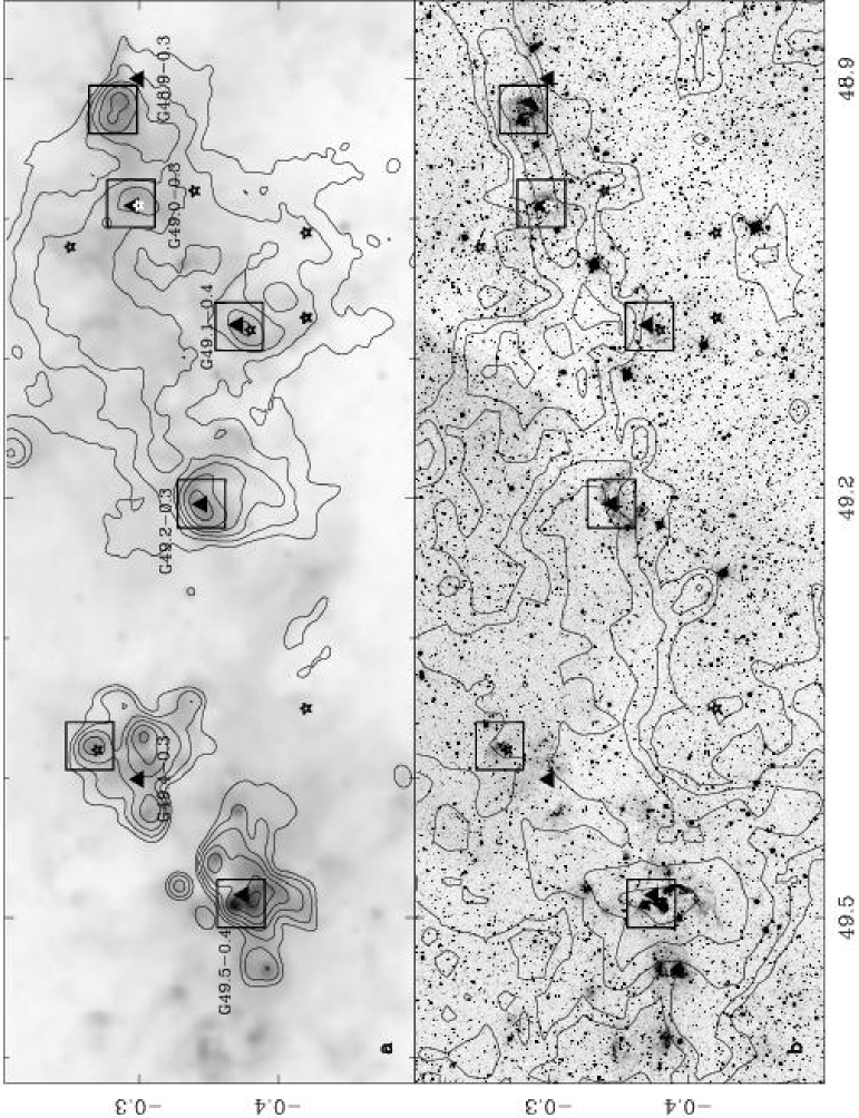
Figure 1: a) MSX A-band (8$\mu$m) image of the W51 GMC, displayed on a logarithmic scale, overlayed by 21 cm continuum contours (Koo & Moon, 1997). The contour levels are 0.1,0.2,0.4,0.8 and 1.6 Jy beam^-1. b) 2MASS $K$-band image of the same region overlayed by contours of ¹³CO integrated intensity (Carpenter & Sanders, 1998). Contour levels are 8,16,32 and 64 K km s^-1. The square boxes mark the observed regions, triangular symbols show the positions of associated UCHII regions and the star symbols represent the IRAS sources that satisfy the Wood & Churchwell (1989) criteria.

2 Observations and Data Reductions

Near-Infrared (NIR) observations were made at the 3.8 m United Kingdom Infrared Telescope (UKIRT) with the facility imager UFTI. The UFTI pixel scale measures 0.091$\arcsec$; the available field of view is $\sim 90\arcsec$. Photometric observations through $JHK$ broad band filters were secured for six fields during three nights of service observing (15 Sep 2000, 31 May 2001 and 12 Aug 2001). Total exposure times in the $J$, $H$ and $K$ filters were 180, 180 and 360 seconds respectively on each of the target fields. The seeing varied between 0.32$\arcsec$ to 0.9$\arcsec$ with a mean of 0.5$\arcsec$ in the $K$-band for the photometric data. A nine point (3$\times$3) jittered observing sequence was executed to obtain data that provided final mosaics with a total field of view of $\sim$115$\arcsec\times$115$\arcsec$. We note that the signal-to-noise ratio at the edges of these mosaics are lower than that within the central 90″area. Standard data reduction techniques involving dark subtraction and median-sky-flat-fielding was applied.

We used tasks available under iraf for photometric analysis. daofind was used to identify sources in each image. A threshold equal to four times the mean noise of each image was found to be sufficient for this purpose. A psf model was computed by choosing several bright stars well-spaced out in the image. Photometry was performed using daophot. Aperture corrections were determined by performing multi-aperture photometry on the psf stars. The instrumental magnitudes were calibrated to the absolute scale using observations of UKIRT faint standards (FS29,FS35 & FS149) that were obtained at airmasses closest to the target observations. The resulting photometric data are in the natural system of the Mauna Kea Consortium Filters (Simons & Tokunaga, 2002). For the purposes of plotting these data in Fig.4 and Fig.5 we have converted them to the Bessell & Brett (1988) (BB) system, since the main-sequence references are in the BB system. Since the direct transformation equations between the Mauna Kea system and the BB sytem are not established as of now, we first converted the Mauna Kea system to CIT system and then to the BB system using equations given by Hawarden et al. (2001). We note that this indirect method can induce high errors for extremely red objects. Representative sub-images of G48.9-0.3 and G49.5-0.4, consisting of stars and nebulosity, were chosen for determining the completeness limits. Limits were established by manually adding and then detecting artificial stars of differing magnitudes. By determining the fraction of stars recovered in each magnitude bin, we have deduced 90% completeness limits of 18.2, 16.9 and 17.3 in the $J$, $H$ and $K$ bands respectively. Our observations are absolutely complete (100%) to the level of 16.2, 14.4 and 15.8 magnitudes in $J$, $H$ and $K$ respectively. The relatively higher detection level in $K$ is due to the fact that the exposure times were twice that in the $J$ & $H$ bands. The photometric accuracy of data presented here is generally $<$0.2 mag although more than 30% of the data points presented in electronic tables have magnitude errors less than 0.05 mag. Astrometry for each of the images was calibrated by using the 2MASS as reference. The astrometric accuracy of the data presented in this paper is better than 0.5″.

Table 1: Summary of observed fields

	Coords(J2000)		PSF	Number of Stars
Name	RA	DEC	″	J	H	K	JHK
G48.9-0.3	19:22:14	14:03:09	0.36	662	1359	2071	593
G49.0-0.3	19:22:26	14:06:46	0.50	954	1659	1757	702
G49.2-0.3	19:23:02	14:16:41	0.90	469	882	905	293
G49.4-0.3	19:23:05	14:28:07	1.10	542	702	744	304
G49.5-0.4	19:23:40	14:31:07	0.32	651	977	1865	529

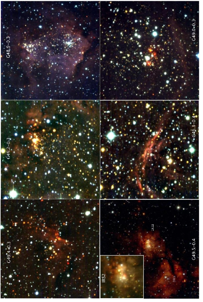
Figure 2: JHK color composites of W51 Embedded clusters

3 Embedded clusters in W51 GMC

We imaged six fields along the W51GMC as represented by the bold, square boxes in Fig. 1. The color plate in Fig. 2 displays JHK band three color composites of each of the observed fields. Regions are referred to using the nomenclature of the associated UCHII region. The images are displayed on a linear scale except for the field G49.5-0.4 which is shown with a logarithmic scale to reveal the central region. As can be seen from Fig. 2, five of these six fields possess clusters of stars immersed in $K$-band nebulosity. The definition of a cluster here implies: (1) a significant increase in the stellar density with respect to an adjacent background, and (2) association with radio continuum sources. The field around G49.5-0.4 is associated with the clusters known as W51 IRS1 and IRS2 (Goldader & Wynn-Williams, 1994). The remaining four clusters are newly discovered from the observations presented here. The star symbols in Fig. 1 mark the positions of IRAS sources that satisfy the Wood & Churchwell (1989) criteria for UCHII regions. Three of these IRAS sources are associated with embedded clusters; the remaining are unassociated with any NIR counterparts. The geometrical coincidence of the observed clusters with the ¹³CO contours and the 21 cm contours indicate that these regions are “embedded” in the gas and dust of the W51 GMC. Table. 1 summarizes the positions and statistics for the five fields, derived from our JHK band photometric analysis. These numbers do not reflect the actual number of stars that belong to the clusters. Our photometric observations provide statistically meaningful data for only four of the five observed clusters; we therefore present detailed analysis only for these four clusters. The regions of G49.4-0.3 and G49.1-0.4 are not included in the detailed analysis presented below.

3.1 Notes on individual clusters

The four embedded clusters discussed below are associated with bright FIR and radio continuum emission. They are, in their own right, interesting objects for detailed high resolution studies at various wavelengths.

G49.5-0.4: This HII region complex is composed of two major components known as W51d and W51e, which are associated with two embedded clusters identified by the prominent infrared sources IRS2 and IRS1(see Fig. 1) The brightest region, W51d, is well-studied at centimeter, millimeter and infrared wavelengths. W51d/IRS 2 is now known to be a young embedded star cluster that is larger and more luminous than the Orion-Trapezium cluster. It contains the water maser complex W51N (Forster & Caswell, 1989), several OH and SiO maser sources (Caswell (2003);Fish et al. (2003)) and is thought to contain several O type young stars. In Fig. 2, the inset of the G49.5-0.4 panel shows three-color JHK-composite image of the central region of the W51d/IRS 2 cluster which, at a spatial resolution of 0.32″, reveals more details than any other image of this region obtained until now. The region shows bright stars and nebulosity, the nebulous cloud appearing to be pinched off to form two lobes stretched east-west. These are called IRS2E and IRS2W and are shown to have electron densities of 10⁵-10⁶ cm^-3(Okumura et al., 2001). Our observations show that IRS2E is associated with a dense cluster, while IRS2W is relatively devoid of stars. Further, the high-resolution view suggests that IRS2E and IRS2W are probably two massive star forming clumps bound by a Roche-lobe potential. The central region is associated with 6-7 mid-infrared point-sources (Kraemer et al., 2001; Okamoto et al., 2001), 6 of which appear as point sources in our high-resolution NIR image. One of the sources appears as a red nebulous condensation (the brightest star of the western blob in the inset) and corresponds to the source KJD3 (Kraemer et al., 2001) which is known to be associated with deep silicate absorption features. Most of these mid-infrared sources are thought to be O-type stars, although there is some debate about whether they are O5-O6 or O9 type stars (Okamoto et al., 2001).

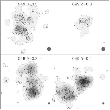
Figure 3: Stellar surface density contours generated by Nyquist binning K-band star counts. The dotted curves with grey shades represent the boundaries of the clusters and are obtained by using a binwidth of 7″. The levels of the dotted contours begins at 4 stars/pixel(7$\arcsec$) and increase in steps of 2 stars/pixel. The solid curves represent the hidden structure of these clusters and are revealed by using smaller bin-widths represented by the grey circles in each panel.

G48.9-0.3: This source is associated with one of the most spectacular clusters discovered in the W51GMC. The top right panel in Fig. 2 display the three color composite of this newly discovered embedded cluster. This cluster is located towards one edge of the $\sim$100 pc long 68km s^-1molecular cloud. It appears to be placed on the tip of the molecular cloud and the observed HII region W51B. High resolution ISOCAM data for this region show strong FIR emission at 6$\mu$m with a morphology similar to the 8$\mu$m MSX data shown in Fig 1. This is a twin cluster immersed in a cradle of nebulosity visible at NIR wavelengths. The southern sub-cluster is a centrally symmetric cluster with a bright white/blue star situated at the geometric center. In contrast, the northern sub-cluster does not have a prominent source, although it does appear centrally symmetric. Indeed, here there appears to be a small ring of stars that is orientated in the plane of the sky.

G49.2-0.3: This is the strongest UCHII region found in the W51B region and corresponds approximately to the location where the shock from the W51C supernova remnant is thought to be interacting with the W51 GMC (Koo & Moon, 1997). It is associated with a group of bright red stars located at the boundary of a cometary shaped HII region. The K-band (red) nebulosity has a similar morphology and is found to be well aligned with the radio free-free emission shown in Fig. 1. Unfortunately, our photometric data for this region suffers from relatively poor seeing (0.9$\arcsec$) and a tracking error which does not allow us to effectively resolve the otherwise dense group of faint sources that is enclosed by the cometary shaped HII region.

G49.0-0.3: The bottom right panel of Fig. 2 shows the three color composite of this field. This region of the W51GMC is bright at 6-8$\mu$m and is relatively weak in terms of radio continuum emission, probably indicating a younger cluster and weaker HII region in comparison with other brighter sources in the W51B region. A faint “bow” of K-band nebulosity, that is similar in morphology to the associated radio continuum emission, surrounds the cluster. This is probably a photo-dissociation region. Our three-color image shows a bright red star centrally-located in the cluster. Also found are two knots of K-band (red) nebulosity in the central region that can not be easily related to any particular star.

3.2 Spatial distribution of stars

It is evident from Figure.1b that the spatial distribution of near-infrared sources is non-uniform, on the global scale of the GMC and also on the local scale of the individual clusters. In order to study the nature of this distribution it is necessary to construct star count surface density maps (SDMs). Such maps provide quantitative estimates of stellar surface densities and their variation across the clusters. They also reveal details about the nature of star formation and the hierarchical structure. Different methods of generating such maps have been followed in various studies of nearby young star clusters. While Lada & Lada (1995) use overlapping rectilinear grids of boxes separated by Nyquist criteria to count the sources in the IC348 cluster, Hillenbrand & Hartmann (1998) bin the source counts into 10$\arcsec$ pixels and smooth the resulting map with a symmetric gaussian profile with a 3-pixel width to produce stellar surface density maps of the Orion Nebula Cluster.

Figure 4: Colour-colour diagrams for four clusters. The solid and broken heavy curves represents the main-sequence dwarf and giant stars, respectively, and the dashed parallel lines are the reddening vectors that enclose reddened main-sequence objects. The crosses on the reddening vectors are separated by A_v=5 magṪhe dotted line indicates the locus of T-Tauri stars (Meyer et al., 1997) and the dotted curve represents the HAeBe locus (Lada & Adams, 1992). The star symbols in the bottom left panel represent the sources in the W51 IRS2 region.

In the above cases the targets of study were nearby star forming regions within 500 pc distance where meaningful source counts could be obtained over projected angular areas of several arcminutes. Massive star forming regions like W51 are generally at much large distances and thus subtend relatively small angular sizes making it difficult to study star count distribution. In these cases spatial resolution plays an important role in the extraction of meaningful information from the SDM. The sizes of individual features we may expect to see on the SDMs depends on the Full-Width Half Maximum (FWHM) of the Point Spread Function (PSF), the binning size adopted to generate the SDMs and the count level itself. Together, these determine whether or not a meaningful SDM can be made. The binning size is a smoothing factor that has to be carefully chosen in such a case. While a small bin size can include just a few sources and not provide a meaningful SDM, an overly large bin size can hide the true features in the SDMs. Given the high quality of the seeing (0.32$\arcsec$) in the $K$-band images of two fields, we experimented with different bin sizes corresponding to 6, 9, 12, 15, 18 and 22 times the FWHM of the PSFs. We found that while the majority of identifiable features did not vary significantly between 6 and 12 times FWHM, the features began to get smeared for a bin size larger than 12 times FWHM. However, to identify the boundaries of the overall cluster and estimate its physical characteristics, a much larger bin size, to smooth all the features, had to be employed.

In Figure. 3 we show SDMs for four fields where the detected source counts were sufficient to produce such a map. We have adopted the method of Lada & Lada (1995) who use a rectilinear grid of overlapping squares separated by half the width of individual squares to provide Nyquist sampling of the sources. We counted all sources from the $K$-band photometry within our completeness limits discussed in the previous section. The cutoff $K$ magnitude for this choice was 17.8 (85% detection limit); the magnitude errors were less than 0.3 mag. The dotted contours and grey shades in Fig. 2 indicate source distribution as obtained by a large smoothing box (150 pixels $\sim$ 14$\arcsec$). These contours are used to identify the cluster boundaries and estimate the average surface density of each cluster. The thick contours overlayed on the grey shades represent SDMs generated by using a smaller binsize (14 $\times$ PSF) that shows smaller groups within these clusters. All the four clusters reveal a clumpy distribution of the NIR sources and the clumps are found to be either elliptical or circular in shape. The elliptical clumps are particularly noticeable in the maps of G48.9-0.3 and G49.5-0.4. The projected dimensions of these clumps are approximately 0.1–0.2 pc. Using the SDM generated with large bins (smooth maps), we estimated the number of stars and the stellar surface densities for each cluster listed in Table. 2.

Figure 5: Color-magnitude diagrams for four fields. The vertical solid lines (from left to right) represent the main-sequence curve reddened by 0, 20 and 40 magnitudes respectively. The horizontal parallel lines represent reddening vectors.

4 Color-Color(CC) and Color-Magnitude(CM) diagrams

Table.1 lists the number of stars detected in each of the J,H and K photometric bands, and simultaneously in all three bands, for each of the fields. For the purposes of photometric analysis of the clusters, we chose all those stars with photometric errors less then 0.2 mag. Tables.2-5 list the astrometry(RA, DEC) and photometry (magnitudes and errors for each of the J, H and K bands) of the stars in sources G48.9-0.3,G49.0-0.3,G49.2-0.3 and G49.5-0.4 respectively. For the four clusters with SDMs in Fig. 3., the stars detected in all three photometric bands are plotted on JHK color-color diagrams in Fig.4. The solid and broken heavy curves represents the main-sequence dwarf and giant stars, respectively, and the dashed parallel lines are the reddening vectors that enclose reddened main-sequence objects.Okumura et al. (2000) estimated the slope of reddenning vector in the direction of W51 to be $\sim$1.9. Similar results are obtained by using 2MASS data. We therefore assumed a reddenning vector slope E(J-H)/E(H-K)=1.9 (BB system) towards W51 region, which relates to an interstellar reddening law with a value of R=3.12 (Whittet & van Breda, 1980). The dotted line indicates the locus of T-Tauri stars (Meyer et al., 1997) and the dotted curve represents the HAeBe locus (Lada & Adams, 1992). Stars that lie outside the region of reddened main-sequence objects are young stellar objects (YSOs) with intrinsic color excesses. By dereddening the stars (on the CC diagrams) that fall within the reddening vectors encompassing the main sequence stars and giants, we found the visual extinction to each star. We de-redenned the stars to the K6-M6 part of the sequence of stars. The individual extinction values range from 0 to 14 magnitudes. From a histogram of these values, we estimate the average foreground extinction to each of the clusters. Two of the clusters (G48.9-0.3 & G49.0-0.3) show two prominent peaks of extinction on the histogram corresponding to the two groups of points that can be identified on the CC diagram. The estimated values of extinction are listed in Table. 2.

It can be noted from Fig. 4 that there are significant differences between the stellar population of the four clusters. G49.0-0.3 and G48.9-0.3 shows two distinct groups of points on the CC diagram separated by about 5-10 magnitudes of visual extinction. In contrast G49.2-0.3 and G49.5-0.4 do not show such distinct groups. Nearly 90% of the points that belong to G49.0-0.3 lie in the region of intrinsically reddened objects, thus signifying a high fraction of YSOs. Further, it appears that G49.0-0.3 has two groups of YSOs, one group more reddened than the other. We found that these two groups of YSOs are distributed homogeneously over the cluster area. Thus the more reddened group is likely embedded in the molecular clump while the least reddened group is probably partially out of or in front of the clump. The bright red star in G49.0-0.3 (see Fig. 2) at the center of the cluster shows colors similar to a T-Tauri star and is highly reddened (A${}_{v}\sim$35 mag). This could be a massive star embedded in this cluster-forming core.

In G48.9-0.3 there is a good mixture of both main-sequence and YSO populations. However, unlike G49.0-0.3, the two groups in this case are found to be distributed differently. The reddened group of stars are all found to occupy the central parts of the two (northern and southern) sub-clusters (see Fig. 2), while stars without much reddening are found to be distributed over the entire FOV of the image. Therefore the average extinction value derived from the reddened group of stars is a good representation of the visual extinction to the molecular clump that hosts the two clusters.

The G49.5-0.4 colour-colour diagram shows mostly main-sequence objects. There is a small percentage of YSOs with varying degrees of reddening. The star symbols in Fig. 4 mark the positions of the stars associated with IRS2 (which is shown inset in the bottom-left panel in Fig. 2). These stars are thought to be O-type stars. The placement of these sources in the upper-right part of the CC diagram supports the conjencture that these are indeed O-type stars (Lada & Adams, 1992). Finally, in Fig. 4 G49.2-0.3 displays very few YSOs and only a few reddened main-sequence objects. If we consider the ratio of sources that fall in the main-sequence zone and the YSO zone as an indicator of the cluster age, then the differences in the CC diagrams discussed above imply that G49.0-0.3 is the youngest cluster in W51, while G48.9-0.3 is the second youngest cluster. In comparison, G49.5-0.4 and G49.2-0.3 are relatively evolved objects.

Table 2: Embedded Clusters in W51 GMC

	Number	Stellar density (pc-2)		Radius(pc)	Age	Av	Mass
Name	of Stars	Average	Peak	($\sqrt{A/\pi}$)	Myr	mag	M⊙
G48.9-0.3	658	175	475	3.43	1.4	(5,10)	10000
G49.2-0.3	505	130	250	3.48	3.0	(6,11)	8000
G49.4-0.3	148	123	175	1.95	2-3	5	2000
G49.5-0.4(IRS1D)	309	221	535	2.09	0.7	5	4400
G49.5-0.4(IRS1E)	333	179	340	2.39	0.7	5	4700

Fig. 5 shows H-K vs K color-magnitude (CM) diagrams for all the four clusters. The vertical solid lines (from left to right) represent the main-sequence curve reddened by 0, 20 and 40 magnitudes respectively. We have assumed a distance of 6.5 kpc for all the clusters, and respective A_v values (listed in Table.1) to each cluster in order to appropriately reproduce the main sequence data on this plot. Similar to the CC diagrams, the CM diagrams show clear differences between the four clusters. The reddened MS stars are found to be spread parallel to the MS line. Clusters G49.5-0.4, G48.9-0.3 and G49.2-0.3 clearly displays this concentration of MS points, which is almost completely absent in the G49.0-0.3 cluster. This agrees well with the results from the CC diagram for G49.0-0.3, i.e. that YSOs comprise about 90% of the total membership of this cluster. The CM diagram of G48.9-0.3 shows the YSOs and MS stars well separated. Points that lie in the upper right corner of the CM diagram (above the line corresponding to O5) represent good candidates for massive YSOs. The relative number of such points are highest in G49.5-0.4, followed by G49.2-0.3 and G48.9-0.3. In contrast, G49.0-0.3 has almost all of its points concentrated in the lower right corner of the CM diagram, corresponding to a population of essentially low mass stars. However, an estimation of the true spectral type of each star can not be made using the CM diagram alone, and warrants NIR spectroscopic observations of the individual sources.

5 Discussion

5.1 Estimating Cluster Properties

In Table.2 we summarise some of the estimated properties of the four embedded clusters in the W51GMC. These estimates are based on the photometric analysis presented in previous sections and some standard methods. The clusters and their boundaries were identified using the SDMs shown in Fig. 3. The stars that fall within the outermost contours shown in Fig. 3 (dotted contours and grey shades) were counted to estimate the number of stars in the cluster. However, the stellar surface density (average and peak values) were estimated by using the star counts within the contour equal to half the peak value. It is clear from Fig. 3 that the clusters are not circularly symmetric and indeed have irregular clumps. The projected area of the clusters were used to define an equivalent radius for the cluster as R=$\sqrt{A/\pi}$, where A is the estimated area of each cluster from Fig. 3. We have estimated a mass for each cluster based on the method described by Lada & Lada (2003). Following this method, we have assumed the K-luminosity function (KLF) models of the Orion Trapezium Cluster (Muench et al., 2002) as a template and used the evolutionary tracks of DÁntona & Mazzitelli (1994) in computing the estimated masses. We have used an age of 1Myr, distance of 6.5Kpc and an average foreground extinction of A_v$\sim$7 mag to compute the masses. The effect of age on the mass of the cluster is such that ages $\leq$1-2Myr yield lower masses compared to ages $\geq$1-2Myr, with all other parameters fixed. However, these assumptions are fair, given the uncertainties involved in our assumed parameters. The estimated mass for the G49.5-0.3 region (IRS1 and IRS2) together is 9100M_⊙  which is similar to the mass estimated by Okumura et al. (2000) for this region (8200M_⊙) who assumes a Salpeter mass function. Our higher estimate is as expected because the spatial sampling here is a factor of 5-6 better compared to Okumura et al. (2000), thus revealing a larger number of cluster members. We also note that the estimated masses are quite sensitive to the assumed extinction values, particularly for distant sources such as these. Therefore, the estimated masses can be uncertain by a few thousand solar masses.

The age of a cluster is one of the most difficult parameters to estimate with our present knowledge because of both observational difficulties and theoretical uncertainties (See Lada & Lada (2003) for a discussion of this problem). In the case of massive star forming regions, some authors use the age of the associated HII regions as an indication of the age of the associated groups of stars. For example, Okumura et al. (2000) give such ages for the four regions falling in the region of W51A. Extending this method to the entire W51GMC region, one finds that the G48.9-0.3 is older than G49.5-0.4(IRS2). From the studies presented here, if we consider the ratio of YSOs to MS stars in each cluster as an indicator of its youth, and also consider the ages indicated by the CM diagrams, it turns out that the IRS2 region is older than the G48.9-0.3 region. This contradicts the result obtained by comparing the ages of the HII region. It has been suggested that the UCHII region phases of massive stars last for a time period much longer than 10⁵yrs if they are born in dense and hot regions (de Pree, 1995). This is because the pressure exerted by the surrounding environment holds the expansion of the UCHII region phase. It may even be possible that massive star formation took place at a much later stage than the low mass star formation (Herbig (1962); Stahler (1985)). Therefore, neither the ages of the massive YSOs, nor the ages of the associated HII regions, are good indicators of the age of the associated embedded clusters.

5.2 Hierarchical and triggered star formation in W51GMC

The studies presented here indicate the existence of at least two, and possibly three, levels of hierarchy in the W51GMC. From Fig. 1 it is evident that star formation has occurred in two major clumps, known as W51A and W51B, within a $\sim$100pc-long molecular cloud. These clumps need not be real and could indeed be the effect of disruption by the supernova remnant W51C (see Koo & Moon (1997) for a detailed discussion). The infrared image of the W51A region shows several clumps that are found as associations of stars and nebulosity (see Fig. 1 of Hodapp & Davis (2002)). Next, as seen in Fig. 2, there is clustering within each of the four clusters. In particular, if we consider the example of G48.9-0.3, which is a double cluster, there appears to be an additional level of hierarchy. All of the clusters, at various levels, indicate hierarchical clustering. Hierarchical structure is believed to be a direct consequence of turbulent energy that operates similarly at different scales (See, e.g., reviews by Elmegreen et al. (2000) & Mac Low & Klessen (2004)). Thus the observed hierarchical clustering indicates the presence of significant turbulent energy in W51GMC which is not yet dissipated. The observed star formation has therefore taken place in the presence of strong turbulent energy.

If we sum-up the mass of all of the clusters listed in Table. 2 we find a total stellar mass of $\sim$30,000M_⊙. Our observations probably represents only $\sim$50% of the total star formation in the W51GMC, due to various reasons. Firstly, we have not sampled all the smaller associations/clusters that can be seen in a large scale 2MASS K-band image. Next, our observations have poor spatial resolution for two of the major clusters; this results in an overly undersampled cluster membership for each cluster. Also, the distributed component of individual young stars across the cloud can contribute a significant percentage to the stellar mass which is neglected. Thus, the total mass estimates from these clusters alone are lower limits. In view of these uncertainties, it may not be unreasonable to assume that the overall star formation in the W51 GMC is associated with a mass of $\sim$5-6$\times$10⁴M_⊙. In such a case, the estimated mass of the W51GMC, $\sim$10⁶M_⊙, derived from observations of the molecular cloud itself (CS98), implies a star formation efficiency (ratio of stellar mass to cloud mass) of $\sim$5-6%. CS98 showed that four of the radio continuum sources, namely G48.9-0.3, G49.0-0.3, G49.1-0.4 and G49.2-0.3, are spatially and kinematically associated with the 68km s^-1cloud alone. If we believe that all the observed clusters in W51 GMC do indeed belong to the 68km s^-1cloud, then the mass estimate of $\sim$2$\times$10⁵M_⊙ for the 68km s^-1cloud (CS98) , together with the mass estimates for the clusters in Table. 2, indicates star formation efficiencies $\sim$10-15%. This value is comparable to the star formation efficiencies in some relatively nearby massive star forming clusters, such as NGC6334 (25%)(Tapia et al., 1996) and W3 IRS5 (6-18%) (Megeath et al., 1996).

Low mass star formation in the solar neighbourhood is known to have a low efficiency, of the order of 1-3%. Triggering mechanisms are thought to result in the formation of clusters; they are also thought to be associated with higher star formation efficiencies. In the W51GMC, the embedded clusters are distributed inside a $\sim$100pc-long cloud. The clusters also likely have ages of 0.5-3 Myrs because that is the commonly observed ages of observed embedded clusters (Lada & Lada, 2003). This suggests near-simultaneous star formation across the entire cloud, an event which could have been spontaneous and/or triggered by an external mechanism. If a triggering mechanism was involved then it would have to have been a large scale shock wave to influence the 100 pc-long region. Internal trigger mechanisms are very unlikely in this case, since the crossing time for the cloud, for an average velocity of $\sim$10km s^-1, is $\sim$10 Myr, which is larger than the typical life time of 3-5 Myr for the embedded clusters. When we consider these facts and note the location of the W51GMC at the tangent point of the Sagittarius spiral arm (Burton, 1970), it seems likely that the observed star formation in the W51GMC is triggered by galactic spiral density waves. Giant clouds like W51 are indeed thought to undergo gravitational collapse under the influence of spiral density waves (Elmegreen, 1994). Therefore, W51GMC may be one of the best examples in our galaxy of triggered star formation by spiral waves.

6 Summary and Conclusions

We present sub-arcsecond resolution, near-infrared J,H,K band photometric observations of six fields in the W51 GMC (which includes the W51A and W51B regions). We construct a multi-wavelength view of the W51 GMC, combining CO and $\lambda$21cm observations from the literature with MSX and 2MASS data. All of these observations together suggest a unified view for W51, the HII regions being associated with a $\sim$100 pc long molecular cloud named the “68km s^-1” cloud by Carpenter & Sanders (1998). The results of our near-infrared observations can be summarised as follows.

1)From our observations of six regions, four new, embedded clusters are discovered that are associated with the UCHII regions G48.9-0.3, G49.0-0.3, G49.2-0.3 and G49.4-0.3. Among these, the cluster associated with G48.9-0.3 is found to be a twin cluster enclosed in a nest of near-infrared nebulosity. Our observations also provide a sub-half arcsecond view of the W51 IRS2 (G49.5-0.4) region that is known to be forming several O-type stars. This high resolution image provides a view which suggests that the W51 IRS2E and IRS2W are two massive star forming clumps that are likely connected by a Roche-lobe potential.

2) Using K-band star counts, we construct stellar surface density maps for four clusters, (G48.9-0.3, G49.0-0.3, G49.2-0.3 and G49.5-0.4.) These maps unveil the underlying hierarchical structure and allow us to estimate some physical parameters for the clusters. Color-color and color-magnitude diagrams for each of the clusters indicate distinct differences in their embedded stellar population. The clusters associated with G48.9-0.3 and G49.0-0.3 are found to contain a high percentage of YSOs, suggesting their relative youth in comparision to the other regions studies.

3) Assuming an Orion Trapezium IMF and theoretical pre-main sequence tracks, we estimate the masses of the individual clusters. The combined mass of all the clusters amounts to a net stellar mass of $\sim$10⁴M_⊙ in the W51 GMC. This estimate, when combined with estimates of the molecular cloud mass from Carpenter & Sanders (1998), suggests a star formation efficiency of $\sim$10%.

Finally, the combined view of the W51 GMC, from our new observations and from the literature, suggests that star formation in the W51 GMC is probably triggered by a galactic spiral density wave. Thus, W51 may represent a relatively unique example of massive star formation in our galaxy.

7 Acknowledgments

The United Kingdom Infrared Telescope is operated by the Joint Astronomy Centre on behalf of the U.K. Particle Physics and Astronomy Research Council. The UKIRT data reported here were obtained as part of its Service Programme. We thank John Carpenter for providing the ¹³CO data and Bon-Chul Koo for providing the HI 21cm data for overlays presented in Fig. 1. We also thank the referee Rob Jeffries for useful suggestions. This work was supported by a grant POCTI/1999/FIS/34549 approved by FCT and POCTI, with funds from the European community programme FEDER. This research made use of data products from the Midcourse Space Experiment and from the Two Micron All Sky Survey. These data products are provided by the services of the Infrared Science Archive operated by the Infrared Processing and Analysis Center/California Institute of Technology, funded by the National Aeronautics and Space Administration and the National Science Foundation.

References

- Bessell & Brett (1988) Bessell, M. S., Brett, J. M., 1988, PASP, 100, 1134
- Burton (1970) Burton, W. B., 1970, A&AS, 2, 291
- Carpenter & Sanders (1998) Carpenter, J. M., Sanders, D. B., 1998, AJ, 116, 1856 (CS98)
- Caswell (2003) Caswell, J. L., 2001, MNRAS, 341, 551
- DÁntona & Mazzitelli (1994) DÁntona, F., Mazzitelli, I., 1994, ApJS, 90, 467
- de Pree (1995) de Pree, C. G., Rodriguez, L. F., Goss, W. M., 1995, RMxAA, 31, 39
- Elmegreen (1994) Elmegreen, B. G., 1994, ApJ, 433, 39
- Elmegreen et al. (2000) Elmegreen, B. G., Efremov, Y., Pudritz, R., Zinnecker, H., 2000, in Mannings, V., Boss, A. P., Russell, S. S., eds, Protostars & Planets IV, University of Arizona Press, p. 179
- Fish et al. (2003) Fish, V. L., Reid, M. J., Argon, A. L., Menten,K. M., 2003, ApJ, 596, 328
- Forster & Caswell (1989) Forster, J.R., Caswell,J.L., 1989, A&A, 213, 339
- Goldader & Wynn-Williams (1994) Goldader, J.D., Wynn-Williams, C.G., 1994, ApJ, 433, 164
- Hawarden et al. (2001) Hawarden, T. G., Leggett, S. K., Letawsky, M. B., Ballantyne, D. R., Casali, M. M., 2001, MNRAS, 325, 563
- Herbig (1962) Herbig, G. H., 1962, ApJ, 135, 736
- Hillenbrand & Hartmann (1998) Hillenbrand, L. A., Hartmann, L. W., 1998, ApJ, 492, 540
- Hodapp & Davis (2002) Hodapp, K. W., Davis, C. J., 2002, ApJ, 575, 291
- Koo (1999) Koo, B., 1999, ApJ, 518, 760
- Koo & Moon (1997) Koo, B. C., Moon D. S., 1997, ApJ, 475, 194
- Kraemer et al. (2001) Kraemer, K. E., Jackson, J. M., Deutsch, L. K., Kassis, M., Hora, J. L., Fazio, G. G., Hoffmann, W. F., Dayal, A., 2001, ApJ, 561, 282
- Lada & Adams (1992) Lada, C. J., Adams, F. C., 1992, ApJ, 393, 278
- Lada & Lada (2003) Lada, C. J., Lada, E. A., 2003, ARAA, 41, 57
- Lada & Lada (1995) Lada, E. A., Lada, C. J., 1995, AJ, 109, 1682
- Mac Low & Klessen (2004) Mac Low, M., Klessen, R. S., 2004, RvMP, 76, 125
- Meyer et al. (1997) Meyer, M. R., Calvet, N., Hillenbrand, L. A., 1995, AJ, 109, 1682
- Megeath et al. (1996) Megeath, S. T., Herter, T., Beichman, C., Gautier, N., Hester, J. J., Rayner, J., Shupe, D., 1996, A&A, 307, 775
- Muench et al. (2002) Muench, A. A., Lada, E. A., Lada, C. J:, Alves, J. F., 2002, ApJ, 573, 366
- Mooney et al. (1995) Mooney, T., Sievers, A., Mezger, P. G., Solomon, P. M., Kreysa, E., Haslam, C. G. T., & Lemke, R., 1995, A&A, 299, 869
- Okumura et al. (2000) Okumura, S., Mori, A., Nishihara, E., Watanabe, E., Yamashita, T., 2000, ApJ, 543, 799
- Okumura et al. (2001) Okumura, S., Mori, A., Watanabe, E., Nishihara, E., Yamashita, T., 2001, AJ, 121, 2089
- Okamoto et al. (2001) Okamoto, Y. K., Hirokazu, K., Takuya, Y., Takashi, M., Takashi, O., 2001, ApJ, 553, 254
- Simons & Tokunaga (2002) Simons, D. A., Tokunaga, A. 2002, PASP, 114, 169
- Stahler (1985) Stahler, S. W., 1985, ApJ, 293, 207
- Tapia et al. (1996) Tapia, M., Persi, P., Roth, M., 1996, A&A, 316, 102
- Whittet & van Breda (1980) Whittet, D. C. B., van Breda, I. G., 1980, MNRAS, 192, 467
- Wood & Churchwell (1989) Wood, D. O. S., Churchwell, E., 1989, ApJ, 340, 265