Interpreting the relationship between galaxy luminosity, color and environment

Abstract

We study the relationship between galaxy luminosity, color, and environment in a cosmological simulation of galaxy formation. We compare the predicted relationship with that found for SDSS galaxies and find that the model successfully predicts most of the qualitative features seen in the data, but also shows some interesting differences. Specifically, the simulation predicts that the local density around bright red galaxies is a strong increasing function of luminosity, but does not depend much on color at fixed luminosity. Moreover, we show that this is due to central galaxies in dark matter halos whose baryonic masses correlate strongly with halo mass. The simulation also predicts that the local density around blue galaxies is a strong increasing function of color, but does not depend much on luminosity at fixed color. We show that this is due to satellite galaxies in halos whose stellar ages correlate with halo mass. Finally, the simulation fails to predict the luminosity dependence of environment observed around low luminosity red galaxies. However, we show that this is most likely due to the simulation’s limited resolution. A study of a higher resolution, smaller volume simulation suggests that this dependence is caused by the fact that all low luminosity red galaxies are satellites in massive halos, whereas intermediate luminosity red galaxies are a mixture of satellites in massive halos and central galaxies in less massive halos.

1 Introduction

One of the keys to understanding galaxy formation and evolution lies in understanding the connection between the observable properties of galaxies and the larger scale environments in which they live. High signal-to-noise correlations between galaxy properties and environment have now been observed in many different galaxy surveys of the local universe (Hogg et al. 2003; Blanton et al. 2004; Gomez et al. 2003; Balogh et al. 2003; Goto et al. 2003; Lewis et al. 2002; Kauffmann et al. 2004, and references therein). The biggest challenge (at least at low redshift) thus lies in predicting these correlations theoretically and understanding their physical origin.

Using data from the Sloan Digital Sky Survey (SDSS; York et al. 2000), Blanton et al. (2003b) showed that luminosity and color are the galaxy properties most strongly correlated with environment (defined as the overdensity of galaxies on a scale of $1h^{-1}\mathrm{Mpc}$ around each galaxy), with other properties such as surface brightness or morphology correlating with environment mainly secondarily through their correlation with luminosity and color. Hogg et al. (2003) and Blanton et al. (2004) explored the dependence of environment on these two galaxy properties in detail. They found that for blue galaxies, the environment does not depend on luminosity, but that local density increases with redder color, whereas for red galaxies there is a strong relation between luminosity and local density. Both very bright ($M_{{}^{0.1}\!{r}}\lesssim-22$) and faint ($M_{{}^{0.1}\!{r}}\gtrsim-19$) red galaxies reside predominantly in highly overdense regions, while galaxies at intermediate luminosities reside in less overdense environments. These effects have also been seen in the dependence of the galaxy autocorrelation function on color and luminosity (Norberg et al. 2002, I. Zehavi et al. in preparation).

In contemporary theories of galaxy formation and evolution, all galaxies reside in virialized dark matter halos, whether they are field galaxies that occupy their own halo or group and cluster galaxies that occupy a larger mass halo along with other galaxies. The observed properties of galaxies, such as color and luminosity, depend on the mass and assembly history of their dark matter halos. The dependence of these properties on environment thus comes from their correlation with halo mass, as well as the correlation of halo mass and history with the larger scale local mass density. The latter has been studied in N-body simulations and is relatively well understood (e.g., Lemson & Kauffmann 1999). It is convenient to think of the correlation of luminosity and color with environment in these terms, since the problem is reduced to understanding the dependence of luminosity and color on halo mass and formation history. This is the route taken by semi-analytic galaxy formation models (e.g., Kauffmann et al. 1999; Benson et al. 2000) and hydrodynamic simulations have recently been analyzed in these terms (Berlind et al. 2003, Z. Zheng et al. in preparation).

In this paper we compare the observed Hogg et al. (2003) environment vs. luminosity and color relation with that predicted by a cosmological hydrodynamic simulation. Furthermore, we interpret the simulation results in terms of the dark matter halos that galaxies occupy.

2 Simulation

We use a smoothed particle hydrodynamics (SPH) simulation of a $\Lambda$CDM cosmological model, with $\Omega_{m}=0.4$, $\Omega_{\Lambda}=0.6$, $\Omega_{b}=0.02h^{-2}$, $h\equiv H_{0}/(100~{}\mathrm{km~{}s}^{-1}~{}\mathrm{Mpc}^{-1})=0.65$, $n=0.95$, and $\sigma_{8}=0.8$. The simulation uses the Parallel TreeSPH code (Hernquist & Katz 1989; Katz, Weinberg, & Hernquist 1996; Davé, Dubinski, & Hernquist 1997) to follow the evolution of $144^{3}$ gas and $144^{3}$ dark matter particles in a $50h^{-1}\mathrm{Mpc}$ box from $z=49$ to $z=0$. The mass of each dark matter particle is $6.3\times 10^{9}M_{\odot}$, the mass of each baryonic particle is $8.5\times 10^{8}M_{\odot}$, and the gravitational force softening is $\epsilon_{\rm grav}=7h^{-1}\mathrm{kpc}$ (Plummer equivalent).

Dark matter particles are only affected by gravity, whereas gas particles are subject to pressure gradients and shocks, in addition to gravitational forces. The TreeSPH code includes the effects of both radiative and Compton cooling. Star formation is assumed to happen in regions that are Jeans unstable and where the gas density is greater than a threshold value ($n_{H}\geq 0.1{\rm cm}^{-3}$) and colder than a threshold temperature ($T\leq 30,000\,$K). Once gas is eligible to form stars, it does so at a rate proportional to $\rho_{\mathrm{gas}}/t_{\mathrm{gas}}$, where $\rho_{\mathrm{gas}}$ is the gas density and $t_{\mathrm{gas}}$ is the longer of the gas cooling and dynamical times. Gas that turns into stars becomes collisionless and releases energy back into the surrounding gas via supernova explosions. A Miller-Scalo (1979) initial mass function of stars is assumed, and stars of mass greater than $8M_{\odot}$ become supernovae and inject $10^{51}$ergs of pure thermal energy into neighboring gas particles. The star formation and feedback algorithms are discussed extensively by Katz, Weinberg, & Hernquist (1996), and the particular simulation employed here is described in greater detail by Murali et al. (2002), Davé et al. (2002), and Weinberg et al. (2004). The parameters are all chosen on the basis of a priori theoretical and numerical considerations and are not adjusted to match any observations.

SPH galaxies are identified at the sites of local baryonic density maxima using the SKID algorithm, which selects gravitationally bound groups of star and cold, dense gas particles. Because dissipation greatly increases the density contrast of these baryonic components (see e.g., Weinberg et al. 2004, Fig. 1), there is essentially no ambiguity in the identification of galaxies. We retain only those particle groups whose mass exceeds a threshold $M_{b,\mathrm{min}}=5.42\times 10^{10}M_{\odot}$, corresponding to the mass of 64 SPH particles, and the resulting galaxy space density is $\bar{n}_{g}=0.02h^{3}{\mathrm{Mpc}}^{-3}$. This space density corresponds to galaxies brighter than $M_{{}^{0.1}\!{r}}<-18.4$ when integrating the Blanton et al. (2003a) SDSS luminosity function (evolved to redshift zero), corresponding to $L/L^{*}=0.18$. The galaxy properties that we use in this analysis, aside from position and velocity, are the total baryonic mass and the median stellar age (i.e., the look-back time to the point at which half of the stellar mass had formed).

To study the effects of numerical resolution, we also analyze a smaller volume, higher resolution simulation having the same cosmological model. This simulation has $128^{3}$ gas and $128^{3}$ dark matter particles in a $22.222h^{-1}\mathrm{Mpc}$ box, yielding particle masses of $1.05\times 10^{8}M_{\odot}$ and $8.8\times 10^{8}M_{\odot}$ for baryonic and dark matter particles, respectively. The gravitational force softening scale is $3.5h^{-1}\mathrm{kpc}$ (Plummer equivalent). This simulation has eight times higher mass resolution than our main $50h^{-1}\mathrm{Mpc}$ simulation, and the lowest mass galaxies that we consider contain 512 baryonic particles instead of 64. In addition to having higher resolution, this simulation includes an additional piece of physics: a photoionizing UV background (calculated by Haardt & Madau 1996).

3 Comparison to SDSS

Hogg et al. (2003) showed the dependence of environment on galaxy colors and luminosities. In order to compare these results to the predictions of our SPH simulation, we must measure the same quantities in the simulation that were measured from the SDSS data. In Hogg et al. (2003), two different definitions of environment are used. The first, which we call $\delta_{g,1}$, is a deprojected angular correlation function that recovers the real-space galaxy density contrast around each galaxy in a spherical Gaussian filter $e^{-r^{2}/2a^{2}}$ of radius $a=1h^{-1}\mathrm{Mpc}$ (Eisenstein 2003). The second, which we call $\delta_{g,8}$, is a simple redshift-space galaxy density contrast in a spherical top-hat filter of radius $8h^{-1}\mathrm{Mpc}$. In both cases, the central galaxy is not counted in the density measurement.

We approximately reproduce these measurements of environment in the SPH simulation. In order to measure $\delta_{g,1}$ for each SPH galaxy, we compute the real-space density of its neighboring galaxies in a spherical Gaussian filter of radius $1h^{-1}\mathrm{Mpc}$. We then divide that density by $\bar{n}_{g}=0.02h^{3}{\mathrm{Mpc}}^{-3}$, the mean density of galaxies in the simulation cube, and subtract one to obtain the density contrast. In order to measure $\delta_{g,8}$, we first put the SPH galaxies in redshift space assuming that the line of sight direction is along the $z-$axis of the simulation cube. We then compute the density of neighboring galaxies in a top-hat sphere of radius $8h^{-1}\mathrm{Mpc}$ and convert to density contrast as before. We also compute $\delta_{m,1}$ and $\delta_{m,8}$, the density contrast of dark matter around each SPH galaxy using $1h^{-1}\mathrm{Mpc}$ Gaussian and $8h^{-1}\mathrm{Mpc}$ top-hat filters, respectively.

Figure 1: Top panel: Monotonic transformation required to convert the baryonic masses of SPH galaxies to absolute ${}^{0.1}\!{r}-$band magnitudes so that their distribution matches that of SDSS galaxies. The dotted line shows the linear relation between luminosity and baryonic mass. Bottom panel: Monotonic transformation required to convert the median stellar ages of SPH galaxies to ${}^{0.1}\!{(g-r)}$ colors so that their distribution matches that of SDSS galaxies.

We have not computed spectral energy distributions for galaxies in the SPH simulation and thus do not predict luminosities and colors. We therefore use the total baryonic mass of each SPH galaxy as a proxy for its luminosity, and the median stellar age as a proxy for its color. Specifically, we assume that a galaxy’s ${}^{0.1}\!{r}-$band luminosity is a monotonic function of its baryonic mass and that its ${}^{0.1}\!{(g-r)}$ color is a monotonic function of its stellar age, and we find the nonlinear transformations that map the simulated mass and age distributions to the observed Blanton et al. (2003b) SDSS $M_{{}^{0.1}\!{r}}$ and ${}^{0.1}\!{(g-r)}$ distributions. These transformations are shown in Figure 1. The $M_{{}^{0.1}\!{r}}$ magnitudes and ${}^{0.1}\!{(g-r)}$ colors of SPH galaxies that we use henceforth are derived in this way. We could in principle use the star formation histories of the simulated galaxies to compute $M_{{}^{0.1}\!{r}}$ and ${}^{0.1}\!{(g-r)}$ directly, but since the modeling of star formation is crude and affected by finite resolution, we believe that this monotonic mapping procedure is more realistic and allows more accurate interpretation of the observed luminosity-color-environment relation.

Figure 1 shows that the transformation required to convert masses to luminosities is strongly nonlinear and significantly shallower than the straightforward linear relation shown by the dotted line. In other words, assuming a roughly constant stellar IMF, the SPH simulation produces too many high mass relative to low mass galaxies, yielding a mass function that does not cut off steeply enough at the high mass end. This problem has been discussed in previous studies that used the same simulation, and it has been partly attributed to numerical resolution effects (Berlind et al. 2003; M. Fardal et al., in preparation). The strange shape of the color-age transformation is caused by the fact that the SDSS color distribution is bimodal, with a blue peak at ${}^{0.1}\!{(g-r)}\sim 0.5$ and a stronger red peak at ${}^{0.1}\!{(g-r)}\sim 0.9$, whereas the SPH age distribution can be described by a single Gaussian with a peak at $\sim 6.7$ Gyr.

In this study we use the SPH galaxy and mass distributions at a redshift of zero. The SDSS galaxies, however, have a median redshift of $z=0.1$. We have checked the SPH predictions at $z=0.125$ and found that there is no significant evolution out to this small redshift.

Figure 2: Mean galaxy density contrast $\langle\delta_{g}\rangle$ measured in bins of absolute ${}^{0.1}\!{r}-$band magnitude (left panels) and ${}^{0.1}\!{(g-r)}$ color (right panels), where $\delta_{g}$ is measured around galaxies in spherical Gaussian filters of radius $1h^{-1}\mathrm{Mpc}$ (top panels) and spherical top-hat filters of radius $8h^{-1}\mathrm{Mpc}$ (bottom panels). Solid points show results for SPH galaxies, curves show the Hogg et al. (2003) results for SDSS galaxies, and open points show the SPH galaxy results multiplied by the ratio of $\sigma_{8}^{2}$ for SDSS and SPH galaxies. Absolute ${}^{0.1}\!{r}-$band magnitudes and ${}^{0.1}\!{(g-r)}$ colors were assigned to SPH galaxies according to the transformations shown in Fig. 1 and discussed in § 3. Error-bars show the uncertainty in the mean estimated from the dispersion found among the eight octants of the simulation cube.

4 Results

Figure 2 shows the dependences of mean environment ($\delta_{g,1}$ and $\delta_{g,8}$) on color and luminosity for both SPH (solid points) and SDSS (curves) galaxies. One of the most striking differences between the two is that the density contrast around SPH galaxies is almost always lower than that of SDSS galaxies. As discussed by Weinberg et al. (2004), the particular realization of initial conditions in this $50h^{-1}\mathrm{Mpc}$ cube leads to a low amplitude of the dark matter correlation function relative to the average of N-body simulations of this volume. This statistical fluctuation probably accounts for most of the difference between the overall level of density contrasts in the simulation and the data, though the systematic effect of missing power on scales larger than the box could play a role, and it is possible that the simulation assumes too low a value of $\sigma_{8,\mathrm{matter}}$ or predicts an incorrect value of galaxy bias. To reduce the impact of the low clustering amplitude on our subsequent analysis, we multiply all SPH density contrasts by $(\sigma_{8,\mathrm{SDSS}}/\sigma_{8,\mathrm{SPH}})^{2}=1.76$, the ratio of clustering amplitudes of SDSS and SPH galaxies on a $8h^{-1}\mathrm{Mpc}$ scale. This correction brings the SPH density contrast levels up to those of the SDSS on both the $1h^{-1}\mathrm{Mpc}$ and $8h^{-1}\mathrm{Mpc}$ scales (open points in Figure 2).

Overall, there is good qualitative agreement between the predicted and observed environments as a function of luminosity and color. In both cases, all galaxies on average live in overdense regions. Moreover, the SPH simulation successfully predicts that the density contrast around galaxies is independent of luminosity at low luminosities, but increases strongly with luminosity for brighter galaxies. The SPH simulation likewise captures the basic dependence of environment on color: there is a slow rise of density contrast around galaxies as they get redder, followed by a levelling off for the reddest galaxies.

However, Figure 2 also reveals interesting differences between theory and observation, the most notable being that the $1h^{-1}\mathrm{Mpc}$ SPH density contrast upturn occurs at roughly one magnitude fainter than it does in the SDSS. This most likely indicates that the simple transformation from baryonic mass to luminosity shown in Figure 1 is not able to repair the overproduction of massive galaxies in the SPH simulation. In order to obtain the correct luminosity function, the nonlinear transformation pulls many high mass galaxies to low luminosities (relative to the luminosities they would be assigned under a linear transformation), but their environments remain very dense, resulting in the density upturn shifting to lower luminosity. Adopting a simple linear transformation between mass and luminosity would result in the predicted density upturn occurring at the right luminosity, but the luminosity function would then be incorrect. We thus conclude that the simulation is successful in predicting the qualitative behavior of the luminosity-density relationship, but fails to get the luminosity scale right. It is possible that this discrepancy is an artifact of the finite simulation volume, which contains only two clusters of mass $M\gtrsim 3\times 10^{14}M_{\odot}$, but it appears significant relative to the error bars in Figure 2, which are estimated from the dispersion among the eight octants of the cube divided by $8^{1/2}$ to yield the standard error on the mean. No monotonic transformation between stellar mass and luminosity would simultaneously reproduce the observed luminosity function and the luminosity scale of the density upturn, so a more complicated environment dependent error in the stellar masses is needed to fix the discrepancy if it is real. We have tried simply adding a 0.3-magnitude scatter to the mass-luminosity relation in Figure 2, but this does not move the upturn to significantly lower luminosity.

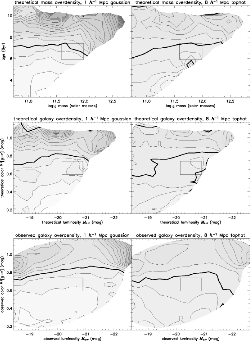
Figure 3: Top panels: Mean dark matter density contrast $\langle\delta_{m}\rangle$ around SPH galaxies measured in sliding rectangular bins of galaxy baryonic mass and median stellar age. The size and shape of the bins are shown in each panel as a rectangular box. Middle panels: Mean galaxy density contrast $\langle\delta_{g}\rangle$ around SPH galaxies measured in sliding rectangular bins of absolute ${}^{0.1}\!{r}-$band magnitude and ${}^{0.1}\!{(g-r)}$ color. Absolute ${}^{0.1}\!{r}-$band magnitudes and ${}^{0.1}\!{(g-r)}$ colors were assigned to SPH galaxies according to the transformations shown in Fig. 1 and discussed in § 3. Bottom panels: $1/V_{max}$-weighted mean galaxy density contrast $\langle\delta_{g}\rangle$ around SDSS galaxies measured in sliding rectangular bins of absolute ${}^{0.1}\!{r}-$band magnitude and ${}^{0.1}\!{(g-r)}$ color. All panels: Left-hand-side panels show densities computed in spherical Gaussian filters of radius $1h^{-1}\mathrm{Mpc}$ and right-hand-side panels show densities computed in spherical top-hat filters of radius $8h^{-1}\mathrm{Mpc}$. In each panel, bold contours show the global mean density contrast and other contours show $20\%$ increments in density contrast (going from lighter to darker regions).

Figure 3 shows the joint mean dependence of environment on color and luminosity. The top panels show the purely theoretical SPH dark matter density contrast as a function of baryonic mass and stellar age. The middle panels show the SPH analog to observations: galaxy density contrast as a function of absolute ${}^{0.1}\!{r}-$band magnitude and ${}^{0.1}\!{(g-r)}$ color, where $M_{{}^{0.1}\!{r}}$ and ${}^{0.1}\!{(g-r)}$ are obtained from the transformations discussed in § 3. Finally, the bottom panels show the observed SDSS galaxy density contrast as a function of $M_{{}^{0.1}\!{r}}$ and ${}^{0.1}\!{(g-r)}$ (first shown by Hogg et al. 2003). Overall there is remarkable agreement between theory and observation, as well as a few notable differences. The main conclusions that we draw from this comparison are as follows:

1. The SPH galaxy density contrast as a function of transformed luminosity and color qualitatively traces the dark matter density contrast as a function of baryonic mass and stellar age. This result is reassuring because it suggests that the observed measurement of environment is likely also tracing the underlying dark matter density.

2. The SPH simulation successfully predicts that the mean density contrast around blue galaxies (${}^{0.1}\!{(g-r)}\lesssim 0.8-0.9$) increases with increasing ${}^{0.1}\!{(g-r)}$ and shows little dependence on luminosity at fixed color.

3. The SPH simulation successfully predicts that very luminous red galaxies reside in highly overdense regions, and that their overdensity increases with luminosity. On the other hand, the simulation underpredicts the luminosity at which the transition to high density occurs. This is the same effect that we saw in Figure 2 and discussed above.

4. The SPH simulation fails to reproduce the observational result that faint red galaxies also reside in highly overdense regions (relative to more luminous red galaxies). Instead, it predicts that red galaxies at $M_{{}^{0.1}\!{r}}\sim-20$ are in highly overdense regions. We show in the next section that this failure is probably an artifact of the simulation’s finite resolution.

5 Discussion

In order to understand the physical origin of the environmental dependences seen in the SPH simulation, it is useful to study them in the context of galaxies occupying dark matter halos. Galaxies that live in high mass halos will always have high density environment measurements simply because their halos contain many other galaxies. Galaxies in low mass halos, however, can only have high density environment measurements if their halos are close to other halos containing galaxies. This means that host halo mass is strongly correlated with measured galaxy environment, and therefore any correlations between galaxy properties and halo mass will also show up as correlations with environment. In order to isolate the halo mass dependence of galaxy colors and luminosities in the SPH simulation, we first identify dark matter halos using a friends-of-friends algorithm (Davis et al. 1985) with a linking length of 0.173 times the mean interparticle separation. We then measure $\delta_{g,\mathrm{in}}$ around each galaxy, which is the component of $\delta_{g,1}$ that only counts galaxies in the same dark matter halo. For a given class of galaxies, the relationship between $\delta_{g,\mathrm{in}}$ and halo mass is thus fully described by $P(N|M)$, the probability distribution that a halo of mass $M$ contains $N$ galaxies of this class (see Berlind & Weinberg 2002 for a thorough discussion of this distribution). This distribution was shown for this SPH simulation by Berlind et al. (2003), as a function of galaxy baryonic mass and stellar population age.

Berlind et al. (2003) also showed that central SPH galaxies within dark matter halos form a distinct population from non-central (satellite) galaxies. In particular, they showed that the central galaxy in each halo is almost always the most massive and often the oldest galaxy in the halo. That result suggests investigating the luminosity-color-environment relation separately for central and satellite galaxies.

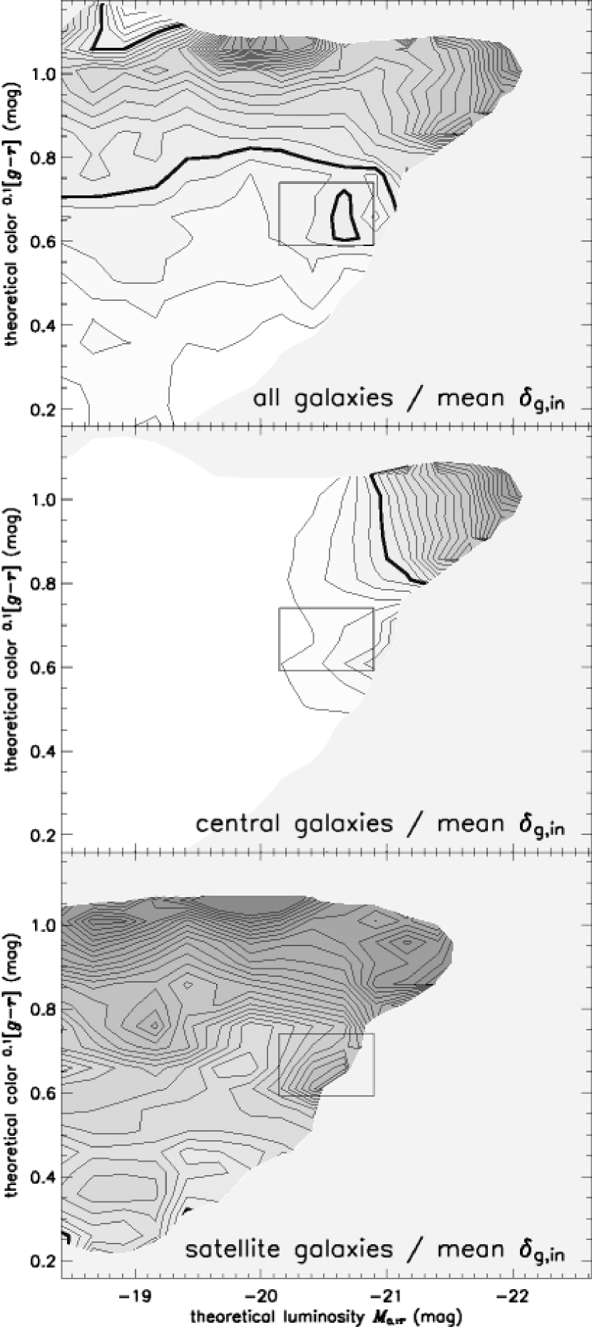
Figure 4: Mean galaxy density contrast $\langle\delta_{g,\mathrm{in}}\rangle$ around SPH galaxies (computed in spherical Gaussian filters of radius $1h^{-1}\mathrm{Mpc}$), counting only galaxies that are in the same dark matter halos as the SPH galaxies around which densities are computed. This relation is shown for all SPH galaxies (top panel), for SPH galaxies that are central in their dark matter halos (middle panel), and for SPH galaxies that are satellites in their dark matter halos (bottom panel). Other features are same as in Fig. 3. Note that though there are no density contours at low luminosities in the middle panel, there are actually many galaxies in that region, but they are mostly isolated single galaxies in halos and thus have a very low, uniform $\langle\delta_{g,\mathrm{in}}\rangle$.

These tests are shown in Figure 4, which plots the mean dependence of $\delta_{g,\mathrm{in}}$ on color and luminosity for all (top panel), central (middle panel), and satellite (bottom panel) galaxies. The striking similarity of the top panel with the middle-left panel of Figure 3, which shows $\delta_{g,1}$ instead of $\delta_{g,\mathrm{in}}$, demonstrates that the environment on a scale of $1h^{-1}\mathrm{Mpc}$ essentially traces the population of the galaxy’s host dark matter halo — galaxies in separate virialized structures make minimal contribution to $\delta_{g,1}$, at least for purposes of this plot. This suggests that the observed Hogg et al. (2003) relation between luminosity, color, and environment is dominated by the underlying relation between galaxy luminosity, color, and dark matter halo mass. Any residual relation with the larger-scale density is not as important.

The middle panel in Figure 4 demonstrates that $\delta_{g,\mathrm{in}}$ (and thus dark matter halo mass) for central galaxies is strongly correlated with luminosity (baryonic mass), and mostly uncorrelated with central galaxy color (median stellar age) at a fixed luminosity. It is not surprising that more massive halos contain more luminous central galaxies, since they have more baryonic mass, and this relation was shown for this SPH simulation by Berlind et al. (2003) (their Figure 18). However, it is interesting that there is little residual relation between halo mass and central galaxy color. This implies that halo mass is much more tightly correlated with central galaxy luminosity than with color. In other words, a fixed mass corresponds to a roughly fixed luminosity, but a broad range in color, thus causing the contours to be vertical. The large scatter in color is probably due to the fact that central galaxy stellar ages are closely related to the formation times of their host dark matter halos, and the distribution of halo formation times for a given mass is broad (e.g., Lacey & Cole 1994; Wechsler et al. 2002). Overall, to the extent that the simulation is representative of the real universe, we conclude that the strong luminosity dependence and weak color dependence of environment for bright red galaxies observed by Hogg et al. (2003) reflects the strong and weak dependences of central galaxy luminosity and stellar population age on halo mass.

The bottom panel in Figure 4 demonstrates that $\delta_{g,\mathrm{in}}$ for satellite galaxies shows the opposite behavior from that of central galaxies: it is strongly correlated with color, and mostly uncorrelated with luminosity at fixed color. Furthermore, comparison to the top panel shows that the environment dependence for galaxies fainter than $M_{{}^{0.1}\!{r}}\sim-21$ tracks that of satellite galaxies. Low luminosity and blue central galaxies live in low mass halos with low $\delta_{g,\mathrm{in}}$, so although they lower the mean $\delta_{g,\mathrm{in}}$ by dilution, the trends of $\delta_{g,\mathrm{in}}$ with galaxy properties are driven by the satellites in more massive halos with higher $\delta_{g,\mathrm{in}}$. The luminosity of a satellite galaxy need not be strongly correlated with its host halo mass, because the galaxy experienced most of its growth while it was the central object of a smaller, independent halo. The strong correlation of satellite color with halo mass probably reflects a combination of two effects: (1) an earlier onset of star formation in high density regions where halos both collapse early and end up merging into massive systems, and (2) the truncation of star formation when a galaxy falls into a larger halo and suffers a reduction of gas accretion. Again, to the extent that the simulation is representative of the real universe, we can conclude that the strong color dependence and weak luminosity dependence of environment for intermediate luminosity, blue galaxies found by Hogg et al. (2003) reflects these trends for satellite galaxies in halos.

While the success of the SPH simulation in reproducing these qualitative trends is encouraging, it is equally interesting that the SPH simulation fails to reproduce the observed environmental dependence for faint red galaxies. Low luminosity galaxies are less well resolved by the simulation and their star formation histories are less accurately modeled; in particular, galaxies close to our adopted $64m_{\mathrm{SPH}}$ resolution threshold have accurate baryonic masses (stars plus cold gas) but artificially low star formation rates and stellar masses because their gas densities are systematically underestimated (M. Fardal et al., in preparation). To test whether the discrepancy with faint red galaxies is an artifact of limited resolution, we analyze the higher resolution, smaller volume simulation described in § 2. Figure 5 shows the joint mean dependence of galaxy density contrast (defined using a spherical $1h^{-1}\mathrm{Mpc}$ Gaussian filter) as a function of absolute ${}^{0.1}\!{r}-$band magnitude and ${}^{0.1}\!{(g-r)}$ color, where $M_{{}^{0.1}\!{r}}$ and ${}^{0.1}\!{(g-r)}$ are obtained from the transformations discussed in § 3. This figure is identical to the middle-left panel of Figure 3, except that it shows the result for the higher resolution simulation. Due to the smaller volume of this simulation, the number of galaxies available is small (there are only 221 galaxies with baryonic masses greater than $5.42\times 10^{10}M_{\odot}$), yielding poor statistics. The number of galaxies is especially low in the high luminosity regime, which is why the environmental dependence for bright red galaxies is not obvious in this figure. Nevertheless, it is clear that low luminosity, red galaxies ($M_{{}^{0.1}\!{r}}\gtrsim-19$, ${}^{0.1}\!{(g-r)}\gtrsim 0.8$) are in highly overdense regions, with higher luminosity red galaxies living in less overdense regions. The results for low luminosity red galaxies in this simulation are much closer to what is seen in the observations (shown in the bottom left panel of Fig. 3). In contrast, the lower resolution simulation lacks the low luminosity red feature and only succeeds in reproducing its high luminosity tail at $M_{{}^{0.1}\!{r}}\sim-20$.

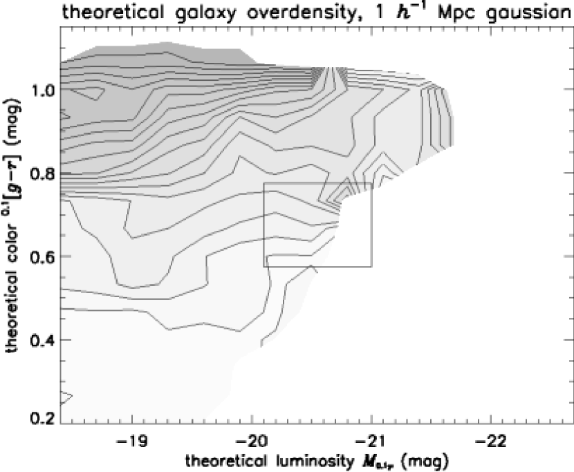
Figure 5: Similar to the middle-left panel of Fig. 3, except that the simulation used is a higher resolution, smaller volume simulation, which is described in § 2.

The $22.222h^{-1}\mathrm{Mpc}$ simulation happens to contain one very massive cluster of galaxies (whose dark matter halo’s viral mass is $\sim 2\times 10^{14}h^{-1}M_{\odot}$). The low luminosity red galaxies that create the overdense feature discussed above are essentially all satellite galaxies of this massive cluster. Low luminosity central galaxies that occupy low mass halos are never old enough to populate the same region of Figure 5 and thus do not dilute the high overdensity signal. As we move to higher luminosities however, the number of satellite galaxies drops drastically because the halos that are large enough to house them become more massive than $M_{*}$ (the characteristic mass scale in the halo mass function). Moreover, at these higher luminosities, isolated central galaxies can be older and thus populate a redder part of the color-luminosity space in Figure 5. They can therefore dilute the high overdensity signal coming from the few intermediate luminosity red satellite galaxies in massive clusters and hence cause the saddle point seen in the figure. This idea, that central galaxies of low mass halos are blue and low luminosity red galaxies must therefore be satellites in more massive halos, is independently supported by the work of I. Zehavi et al. (in preparation), who model the luminosity and color dependence of the two-point correlation function using halo occupation distribution models.

We suspect that spurious scatter in the stellar ages of galaxies near the resolution limit of the lower resolution simulation mixes the populations of low luminosity central galaxies in low mass halos with low luminosity satellites in massive halos and thus erases the low luminosity red galaxy feature. An additional effect of low resolution that could contribute to this problem is overmerging of low mass satellites in massive halos. This would reduce their numbers and consequently their overdensity measurements. The higher resolution simulation also differs from the lower resolution one in that it includes a photoionizing UV background. It is possible that this additional piece of physics contributes to the faint red feature seen in Figure 5, but not in Figure 3 though it would be surprising for photoionization to have an important effect at such a high mass scale. Finally, it is possible (though unlikely) that the faint red feature seen in the SDSS data is caused by other physical mechanisms that are not included in these simulations and that the feature seen in Figure 5 is a statistical fluke resulting from only one unusually red cluster. Similar predictions by semi-analytic galaxy formation models and pure dark matter high resolution simulations should help to resolve this issue.

6 Summary

In sum, these results suggest a straightforward interpretation of the main trends in the environment-luminosity-color relation found by Hogg et al. (2003) and Blanton et al. (2004) in the SDSS.

1. Measurements of local galaxy density around galaxies essentially trace the mass of their underlying dark matter halos. Contributions from neighboring halos are not as important.

2. The environment dependence for luminous red galaxies reflects the trends for central galaxies in massive (cluster sized) halos. The environment depends strongly on luminosity and weakly on color because for central galaxies, these quantities are strongly and weakly correlated with halo mass, respectively.

3. The environment dependence for lower luminosity red galaxies reflects the changing mixture of central and satellite galaxies as a function of color and luminosity. Low luminosity red galaxies are all satellites in high mass halos (whose central objects are luminous red galaxies) — low luminosity central galaxies are always bluer and thus do not populate the same part of the color luminosity space. However, intermediate luminosity red galaxies can be both satellites in very massive halos and central galaxies in low mass halos. They thus reside, on average, in lower mass halos (and consequently in lower density regions) than either their higher or lower luminosity counterparts.

4. The environment dependence for blue galaxies reflects the trends for satellite galaxies in intermediate mass (group sized) halos. For this population, luminosity is only weakly correlated with host halo mass (and thus environment), while color is strongly correlated.

References

- Balogh et al. (2003) Balogh, M. et al. 2003, ApJsubmitted, astro-ph/0311379
- Benson et al. (2000) Benson, A. J., Baugh, C. M., Cole, S., Frenk, C. S., & Lacey, C. G. 2000, MNRAS, 316, 107
- Berlind & Weinberg (2002) Berlind, A. A., & Weinberg, D. H. 2002, ApJ, 575, 587
- Berlind et al. (2003) Berlind, A. A., Weinberg, D. H., Benson, A. J., Baugh, C. M., Cole, S., Davé, R., Frenk, C. S., Jenkins, A., Katz, N., & Lacey, C. G. 2003, ApJ, 593, 1
- Blanton et al. (2003a) Blanton, M. R. et al. 2003a, ApJ, 592, 819
- Blanton et al. (2003b) Blanton, M. R. et al. 2003b, ApJ, 594, 186
- Blanton et al. (2004) Blanton, M. R., Eisenstein, D., Hogg, D. W., Schlegel, D. J., & Brinkmann, J. 2004, ApJ, submitted
- Davé, Dubinski, & Hernquist (1997) Davé, R., Dubinski, J., Hernquist, L. 1997, New Astronomy, 2, 277
- Davé et al. (2002) Davé, R., Katz, N., & Weinberg, D. H. 2002, ApJ, in press, astro-ph/0205037
- Davis et al. (1985) Davis, M., Efstathiou, G., Frenk, C. S., & White, S. D. M. 1985, ApJ, 292, 371
- Eisenstein (2003) Eisenstein, D., J. 2003, ApJ, 586, 718
- Gomez et al. (2003) Gomez, P. L. et al. 2003, ApJ, 584, 210
- Goto et al. (2003) Goto, T., Yamauchi, C., Fujita, Y., Okamura, S., Sekiguchi, M., Smail, I., Bernardi, M., & Gomez, P. L. 2003, MNRAS, 346, 601
- Haardt & Madau (1996) Haardt, F., & Madau, P. 1996, ApJ, 461, 20
- Hernquist & Katz (1989) Hernquist, L., & Katz, N. 1989, ApJS, 70, 419
- Hogg et al. (2003) Hogg. D. W., et al. 2003, ApJ, 585, L5
- Katz, Weinberg, & Hernquist (1996) Katz, N., Weinberg, D. H., & Hernquist, L. 1996, ApJS, 105, 19
- Kauffmann et al. (1999) Kauffmann, G., Colberg, J. M., Diaferio, A., & White, S. D. M. 1999, MNRAS, 303, 188
- Kauffmann et al. (2004) Kauffmann, G., White, S. D. M., Heckman, T. M., Menard, B., Brinchmann, J., Charlot, S., Tremonti, C., & Brinkmann, J. 2004, MNRAS, submitted, astro-ph/0402030
- Lacey & Cole (1994) Lacey, C. G., & Cole, S.1994, MNRAS, 271, 676
- Lemson & Kauffmann (1999) Lemson, G. & Kauffmann, G. 1999, MNRAS, 302, 111
- Lewis et al. (2002) Lewis, I. et al. 2002, MNRAS, 334, 673
- Miller & Scalo (1979) Miller, G. E., & Scalo, J. M. 1979, ApJS, 41, 513
- Mo et al. (2003) Mo, H. J., Yang, X., van den Bosch, F. C., & Jing, Y. P. 2003, MNRASsubmitted
- Murali et al. (2002) Murali, C., Katz, N., Hernquist, L., Weinberg, D. H., & Davé, R. 2002, ApJ, 571, 1
- Norberg et al. (2002) Norberg, P. et al. 2002, MNRAS, 332, 827
- Wechsler et al. (2002) Wechsler, R. H., Bullock, J. S., Primack, J. R., Kravtsov, A. V., & Dekel, A. 2002, ApJ, 568, 52
- Weinberg et al. (2004) Weinberg, D. H., Davé, Katz, N., & Hernquist, L. 2004, ApJ, 601, 1
- York et al. (2000) York, D. G. et al. 2000, AJ, 120, 1579