Multi-Phase Galaxy Formation: High Velocity Clouds and the Missing Baryon Problem

Abstract

The standard treatment of cooling in Cold Dark Matter halos assumes that all of the gas within a “cooling radius” cools and contracts monolithically to fuel galaxy formation. Here we take into account the expectation that the hot gas in galactic halos is thermally unstable and prone to fragmentation during cooling and show that the implications are more far-reaching than previously expected: allowing multi-phase cooling fundamentally alters expectations about gas infall in galactic halos and naturally gives rise to a characteristic upper-limit on the masses of galaxies, as observed. Specifically, we argue that cooling should proceed via the formation of high-density, $\sim 10^{4}$K clouds, pressure-confined within a hot gas background. The background medium that emerges has a low density, and can survive as a hydrostatically stable corona with a long cooling time. The fraction of halo baryons contained in the residual hot core component grows with halo mass because the cooling density increases with gas temperature, and this leads to an upper-mass limit in quiescent, non-merged galaxies of $\sim 10^{11}M_{\odot}$.

In this scenario, galaxy formation is fueled by the infall of pressure-supported clouds. For Milky-Way-size systems, clouds of mass $\sim 5\times 10^{6}M_{\odot}$ that formed or merged within the last several Gyrs should still exist as a residual population in the halo, with a total mass in clouds of $\sim 2\times 10^{10}M_{\odot}$. The baryonic mass of the Milky Way galaxy is explained naturally in this model, and is a factor of two smaller than would result in the standard treatment without feedback. We expect clouds in galactic halos to be $\sim 1$kpc in size and to extend $\sim 150$kpc from galactic centers. The predicted properties of Milky Way clouds match well the observed radial velocity distribution, angular sizes, column densities, and velocity widths of High Velocity Clouds around our Galaxy. The clouds we predict are also of the type needed to explain high-ion absorption systems at $z<1$, and the predicted covering factor around external galaxies is consistent with observations.

1 Introduction

Cooling and galaxy formation within dark matter halos was first discussed in a modern context by White & Rees (1978), who argued that gas cooling was a main driver behind the characteristic mass of galaxies. After halo collapse, gas is assumed to shock-heat to the halo temperature, and to cool over a characteristic timescale

$$\tau_{\rm c}\simeq{{k_{b}T}\over{n_{i}\Lambda(T)}},$$ (1)

which depends on the particle number density of the ionized gas $n_{i}$, the gas temperature $T$, the Boltzman constant $k_{b}$, and the cooling function $\Lambda(T)$. White & Frenk (1991) extended this approach in order to make predictions as a function of time and position in a halo. The framework assumes that all of the gas within a central, high-density “cooling radius” cools and falls in to fuel galaxy assembly, while gas beyond this radius remains hot. This cooling-radius method for tracking gas cooling is certainly a useful approach, and it has become the basis for gas accretion estimates in semi-analytic galaxy formation models (recently, Somerville et al., 2001; Benson et al., 2003; Hatton et al., 2003; Hernquist & Springel, 2003; Nagashima & Yoshii, 2004). Hydro-dynamical simulations seem to verify this picture, at least roughly (Katz, 1992; Thoul & Weinberg, 1995; Springel et al., 2001; Yoshida et al., 2002; Helly et al., 2003).

Implicit in this standard model is that all of the gas within the cooling radius cools and contracts monolithically. It has been known for some time, however, that the hot gas associated with galaxies (and clusters) should be thermally unstable and prone to fragmentation (Field, 1965; Fall & Rees, 1985; Murray & Lin, 1990). At a given radius within a halo, the cooling time can increase for some gas and decrease for other gas as density and temperature differences become enhanced by the cooling process. The result is a fragmented distribution of cooled material, in the form of warm ($\sim 10^{4}$K) clouds, pressure-supported within a hot gas background. In this paper we argue that the consequences of including this expected ingredient may be far-reaching. The residual hot gas core has a low density, and thus can exist as a pressure-supported corona for a long time without cooling. The fraction of baryonic mass contained in the hot core component grows with halo velocity (or temperature) and we show below that this gives rise to a characteristic cooled, central galaxy mass of $\sim 10^{11}M_{\odot}$ in high-mass halos. Interestingly, this is roughly what is needed to explain the bright-end cutoff in the galaxy luminosity function. Similarly, including this multi-phase treatment can help explain the masses of Milky-Way type galaxies without the need for excessive feedback.

In our picture, the gas supply into galaxies is governed by the infall of warm clouds. We suggest that the cloud population will have a velocity dispersion similar to that of the host halo, and that clouds will fall in to feed galaxy formation only when cloud-cloud collisions or ram pressure forces rob them of angular momentum and kinetic energy. In Milky-Way-size halos, the residual population of clouds is expected to be substantial. The clouds occupy typical galacto-centric radii of $\sim 100$kpc, and can explain the High Velocity Cloud (HVC) population around the Milky Way and high-ion absorption systems in external galaxies. A characteristic cloud mass of $\sim 5\times 10^{6}M_{\odot}$ matches most of the observed properties of HVCs (see §7). The same characteristic cloud mass is consistent with our theoretical expectations (§5), aides in the understanding of absorption systems (§8), and helps explain the total mass of the Milky Way without any significant feedback (§6). Based on this evidence, we argue that there is direct observational support for the idea that gas fragmentation be included in models of CDM-based galaxy formation.

In what follows we will use the Milky Way galaxy halo as a fiducial case for comparison. The properties of our “Milky Way” dark matter halo are adopted from results of Klypin et al. (2002). The authors use a wide variety of Galactic data and a baryonic-infall calculation to determine a best-fit halo mass of $M_{\rm v}\simeq 10^{12}M_{\odot}$ and an initial halo maximum circular velocity of $V_{\rm max}=163{\rm km}\ {\rm s}^{-1}$. Their Milky Way mass is motivated by the mass models of Dehnen & Binney (1998), who obtain $M_{G}=(4-6)\times 10^{10}M_{\odot}$.

The results of Klypin et al. (2002) and Dehnen & Binney (1998) also provide a useful illustration of the “over-cooling problem” faced by the standard treatment of cooling in galaxy halos. In the standard model, the baryons that end up in the Galaxy are simply those that exist within the cooling radius: $M_{\rm c}=f_{c}f_{b}M_{\rm v}$. Here $f_{c}\simeq 0.7$ is the fraction of baryonic mass within the cooling radius for Milky-Way type halos (see §3) and $f_{b}=\Omega_{b}/\Omega_{m}\simeq 0.17$ is the cosmic baryon fraction (Spergel et al., 2003). Based on the numbers quoted above, the ratio of the “expected” cooled mass to the actual mass of the Galaxy, $f_{\rm G}=M_{\rm G}/M_{\rm c}$, is significantly less than unity:

$$f_{\rm G}\simeq 0.43\left[\frac{M_{\rm G}}{5\times 10^{10}M_{\odot}}\right]\left[\frac{M_{\rm v}}{10^{12}M_{\odot}}\right]^{-1}\left[\frac{f_{b}f_{c}}{0.12}\right]^{-1}.$$ (2)

If the standard cooling arguments are correct, then less than half of the baryons that have cooled onto the Galaxy still exist there today. If feedback is to explain this, it requires that the Galaxy lost half of its mass via strong winds without destroying the thin disk. In our picture, this difficult series of events is avoided because a large fraction of the mass within the cooling radius never fell in, but remains in the halo in the form of a warm/hot medium (see §6). This effect becomes more important in high-mass halos because the density of the hot gas core (which scales like the cooling density) increases with halo temperature.

We have made an effort to frame our results as an extension of the standard treatment of cooling, and we give comparisons to the single-phase approach whenever possible. Of course, gas cooling and accretion in galactic halos is more complicated than the static halo model we use. Indeed gas falling into halos may or may not be shock-heated efficiently, and some gas was likely accreted as cold material, either stripped from infalling satellites, or simply as “cold flows” (Birnboim & Dekel, 2003; Keres et al., 2004). Our goal is merely to extend the standard semi-analytic treatment to include an allowance for multi-phase gas during cooling and to work out the implications of this approach. We expect that no matter how gas clouds are accreted, our qualitative expectations will hold. Detailed, high-resolution hydrodynamic simulations will be needed to test these expectations. Unfortunately, as we discuss in §11, the numerical challenges facing such an endeavor may be significant.

Symbol	Equation where first used	Description
$f_{b}$	(2)	The fraction of mass in the universe in the form of baryons.
$M_{\rm v},R_{\rm v},V_{\rm v}$	(3)(3)(3)	Halo virial properties: mass, radius, and velocity.
$R_{\rm s},V_{\rm max},C_{\rm v}$	(6) (4) (8)	Halo parameters: NFW scale radius, maximum circular velocity, and NFW concentration.
$\Lambda(T),\Lambda_{z}$	(12) (13)	The cooling function and its approximate metallicity scaling
$\rho_{c},n_{\rm c},R_{\rm c}$	(12) (14) (16)	The cooling density, corresponding electron number density, and cooling radius
$\mu_{i},\mu_{e},Z_{g}$	(5) (12) (13)	The mean gas mass per particle, mean gas mass per electron, and the gas metallicity.
$\eta_{T},\eta_{d},\eta_{P}$	(22) (22) (22)	Ratios of average hot gas core temperature, density, and pressure to the values at the cooling radius.
${\rho}_{w},T_{\rm w}$	(25) (25)	Warm cloud density and temperature.
$m_{\rm cl},r_{\rm cl},\rm v_{cl}$	(25) (26) (37)	Cloud mass, cloud radius, and the typical cloud velocity.
$M_{\rm c},M_{\rm h},M_{\rm cl},M_{\rm g}$	(24) (24) (44) (46)	The total mass in various phases: cooled material, hot core, clouds, central galaxy.
$\tau_{\rm ram},\tau_{cc},\tau_{\rm in}$	(43) (44) (47)	Cloud population time scales: the ram-pressure time, the cloud-cloud collision time, the cloud infall time.

Table 1: Frequently used symbols

Before providing an outline of the paper, we mention that in a series of papers, D. Lin and collaborators (Murray & Lin, 1990, 1992; Lin & Murray, 1992; Murray et al., 1993; Burkert & Lin, 2000; Lin & Murray, 2000; Murray & Lin, 2004) have explored the fate of warm clouds in a hot gas medium. The analysis that follows builds on their work. Mo & Miralda-Escude (1996) consider the presence of pressure-supported clouds in dark matter halos in order to explain QSO absorption line systems. We make a similar connection in §8.

The next section contains a review of the properties of dark matter halos. In §3 we describe the standard treatment of radiative cooling in halos. §4 extends this model to include the formation of warm clouds within a background hot gas medium. In §5 we explore cloud masses, bracket the allowed range, and discuss mass scales of interest. §6 is devoted to modeling galaxy fueling via cloud infall. In §7 and §8 we compare our expected cloud populations to HVC data and CIV absorption system observations, respectively. §9 presents an explanation for the exponential cutoff in the bright-end of the galaxy luminosity function. Future directions and implications are discussed in §10 and we summarize in §11. In what follows, we adopt a flat $\Lambda$CDM cosmology, with parameters set by the best-fit WMAP values: $h=0.72$, $\Omega_{b}h^{2}=0.024$, and $\Omega_{m}h^{2}=0.14$ (Spergel et al., 2003, see also Primack (2002)) The implied fraction of mass in baryons is $f_{b}=0.17$.

2 Dark Matter Halos

A dark matter halo of a given mass $M_{\rm v}$ is characterized by a virial radius $R_{\rm v}$. The spherical top hat model (Gunn & Gott, 1972) provides a reasonable estimate of the value of $R_{\rm v}$, which is set by the radius at which the average mass enclosed equals a characteristic virial density $\bar{\rho}_{\rm v}\equiv\Delta_{\rm v}\rho_{u}$. Here $\rho_{u}$ is the matter density of the universe and $\Delta_{\rm v}$ is a cosmology-dependent variable that can vary as a function of redshift. For our adopted $\Lambda$CDM cosmology $\Delta_{\rm v}\simeq 360/(1+z)$ when $z\lower 2.58334pt\vbox{\hbox{$\buildrel\textstyle<\over{\sim}\ $}}1$ and $\Delta_{\rm v}\simeq 178$ when $z\lower 2.58334pt\vbox{\hbox{$\buildrel\textstyle>\over{\sim}\ $}}1$ (a more precise fit is given by Bryan & Norman, 1998). With this definition the halo virial mass and radius are related via

$$R_{\rm v}=\left({{3M_{\rm v}}\over{4\pi\bar{\rho}_{\rm v}}}\right)^{1/3},\quad V_{\rm v}=\sqrt{\frac{GM_{\rm v}}{R_{\rm v}}}.$$ (3)

The singular isothermal sphere (SIS) is a simple approximation that is often adopted for the density profile of a dark matter halo:

$$\rho(R)={{\bar{\rho}_{\rm v}R_{\rm v}^{2}}\over{3R^{2}}}={{V_{\rm max}^{2}}\over{4\pi G}}{{1}\over{R^{2}}}.$$ (4)

The SIS profile has a rotation curve that is flat as a function of $R$: $V(R)=V_{\rm v}=V_{\rm max}$, where $V_{\rm max}$ is defined to be the maximum rotation velocity of the halo. The temperature of a singular isothermal sphere is related to its velocity by

$$T={{\mu_{i}m_{p}c_{g}^{2}}\over{\gamma k_{b}}}=10^{6}K\left({{V_{\rm max}}\over{163{\rm km}\ {\rm s}^{-1}}}\right)^{2},$$ (5)

where $c_{g}=V_{\rm max}/\sqrt{2}$ is the sound speed of the gas, $m_{p}$ is the proton mass, the polytropic index is $\gamma=1$ for an isothermal gas, and $\mu_{i}=0.62$ is the mean mass per particle (electrons and nucleons) of the ionized gas in units of the proton mass assuming a $30\%$ mass fraction in Helium.

While the SIS is convenient for illustrative purposes, a better fit to the results of cosmological N-body simulations is the NFW profile (Navarro et al., 1995; Klypin et al., 2001)

$$\rho(R)={{\rho_{s}R_{\rm s}^{3}}\over{R(R+R_{\rm s})^{2}}},$$ (6)

where $\rho_{s}$ is a characteristic density. The scale radius, $R_{\rm s}$ is often expressed in terms of the concentration $C_{\rm v}=R_{\rm v}/R_{\rm s}$. Given a halo mass, the value of $C_{\rm v}$ sets the value of $\rho_{s}$, and the profile is determined. Simulations show that the median value of $C_{\rm v}$ for a halo of mass $M_{\rm v}$ at redshift $z$ is well-approximated by $C_{\rm v}(M,z)\simeq 9.6(M_{\rm v}/M_{*})^{-0.13}(1+z)^{-1}$ (Bullock et al., 2001). Here $M_{*}$ $\simeq 10^{13}M_{\odot}$ is the characteristic mass for collapse at $z=0$ for our cosmology (see Lacey & Cole, 1993).

The maximum circular velocity for an NFW profile occurs at a radius $R_{\rm max}\simeq 2.15R_{\rm s}$, where $V_{\rm max}^{2}\equiv GM(R_{\rm max})/R_{\rm max}$. For our adopted cosmology, a good fit to the virial velocity in terms of $V_{\rm max}$ is

$$V_{\rm v}\simeq 0.468V_{\rm max}^{1.1},$$ (7)

which is good to $1\%$ for $V_{\rm v}$ between $80{\rm km}\ {\rm s}^{-1}$ and $1200{\rm km}\ {\rm s}^{-1}$. We assume that in the absence of cooling, the relationship between velocity and temperature for NFW halos follows that for isothermal halos (equation 5).

Finally, N-body simulations show that the mass accretion history of a dark matter halo as a function of redshift $z$ follows a remarkably well-defined function of the final concentration $C_{\rm v}^{0}$ (Wechsler et al., 2002):

$$M_{\rm v}(z)=M_{\rm v}(0)\exp\left[\frac{-8.2z}{C_{\rm v}^{0}}\right].$$ (8)

Galaxy-mass halos have $C_{\rm v}^{0}\simeq 13$, and typically have accreted half of their mass by $z_{f}\sim 1.1$, corresponding to a lookback “formation time” of $t_{f}\simeq 8\rm Gyr$.

As discussed in Wechsler et al. (2002) dark halos tend to grow qualitatively from the inside out (see also Helmi et al., 2003; Zentner & Bullock, 2003; Tasitsiomi et al., 2003). The central density remains roughly constant at the value set during an early, rapid accretion phase of halo buildup. Because of this, for a given halo, $V_{\rm max}$ is relatively constant, as a function of lookback time. Indeed for halos with $V_{\rm max}\simeq 175-250{\rm km}\ {\rm s}^{-1}$ at $z=0$ simulations show that $V_{\rm max}$ stays approximately constant in the main progenitor back to $z\simeq z_{f}$ (R. Wechsler, private communication). Motivated by these results, in what follows we will assume that the halo $V_{\rm max}$ (and thus its temperature) will remain constant back to the time of formation. With these properties of dark matter halos defined we can move on to the treatment of gas in a halo.

3 Hot Gas and Collisional Cooling

In the standard picture of CDM-based galaxy formation, gas collapses with the dark matter, and subsequently shock heats to the temperature of the virialized halo (see White & Frenk, 1991). The result is an extended halo of hot gas, which begins to cool over a characteristic timescale (equation 1), and provides the gas reservoir for galaxy formation. Recently it has been shown in hydrodynamical simulations that the situation is not as simple as this (Birnboim & Dekel, 2003; Keres et al., 2004). In low-mass halos, $V_{\rm max}\lower 2.58334pt\vbox{\hbox{$\buildrel\textstyle<\over{\sim}\ $}}100{\rm km}\ {\rm s}^{-1}$, the cooling time of the gas is so short that a shock can not be maintained. Thus gas accretes in a ”cold flow”. For halos with $V_{\rm max}\lower 2.58334pt\vbox{\hbox{$\buildrel\textstyle>\over{\sim}\ $}}100{\rm km}\ {\rm s}^{-1}$ simulations find that the gas does indeed shock heat to the temperature of the halo. In our multi-phase model of the gas, we can interpret these cold flows as gas that simply enters the halo as warm clouds (without first shock-heating and subsequently re-forming clouds).

In what follows we work within the framework of the standard picture and investigate how the treatment of fragmentary cloud cooling will change the results. We do so mainly in the spirit of direct comparison. Although, as we show below, most of the interesting ramifications of including multi-phase cooling occur in high-mass halos, where shock-heating is expected to occur, and the standard picture is roughly valid. As mentioned in the introduction, different expectations for the nature of gas accretion onto halos and the efficiency of shock heating will affect our results somewhat, but the qualitative nature of our conclusions will not change. For example, gas stripped from infalling halos will likely fragment into clouds during this process, as seen directly in the the Magellanic Stream (e.g. Weiner & Williams, 1996) and lead to a configuration similar to what we discuss below (although via a different chain of events). Of course, more direct modeling will be needed to test these expectations in detail.

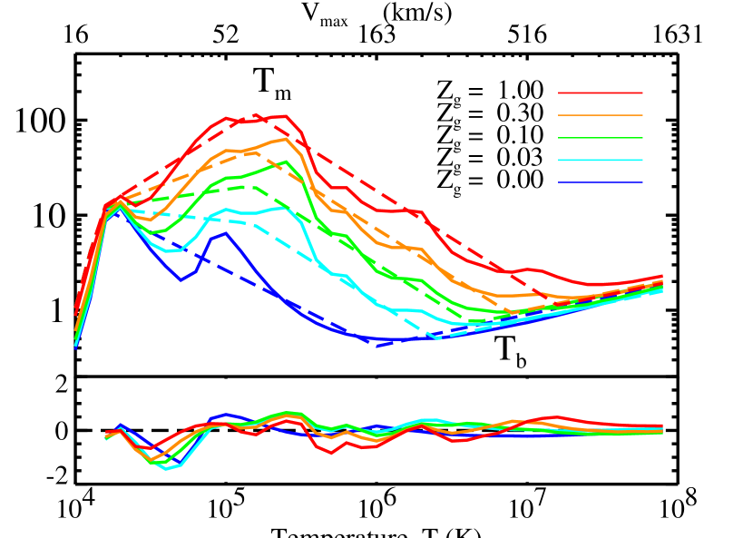
Figure 1: The cooling function for five different metallicities as a function of halo temperature (lower scale) and corresponding halo maximum velocity (upper scale). The five metallicities, from top to bottom, are: $Z_{g}=1.0,0.3,0.1,0.03$ and $0.0$ relative to solar. Also shown are simple power-law fitting functions described in Appendix A for each metallicity (dashed lines). The power laws change slope at two characteristic temperatures, $T_{m}$ and $T_{b}$, corresponding to when metal line and Bremsstrahlung cooling start to dominate, respectively. The fractional difference between the full function and the fit are shown in the bottom panel.

3.1 The Initial Hot Gas Profile

After halo formation, we assume that the hot gas obtains an extended density profile. Motivated by the non-radiative hydrodynamic simulations summarized in Frenk et al. (1999), we assume that a dark halo with an NFW profile and concentration $C_{\rm v}$ will initially have hot gas that traces the DM at large radius, but that develops a thermal core at $\simeq 3R_{\rm s}/4$:

$$\rho_{g}^{i}(R)=\frac{R_{\rm s}^{3}\rho_{0}}{(R+\frac{3}{4}R_{\rm s})(R+R_{\rm s})^{2}},\quad\rho_{0}={{M_{b}}\over{4\pi R_{\rm s}^{3}g(C_{\rm v})}}.$$ (9)

This profile gives a good fit to Fig. 12 in Frenk et al. (1999). The normalization, $\rho_{0}$, is set so that the total initial gas mass within the halo is $M_{b}=f_{b}M_{\rm v}$. The function $g(x)$ describes the radial gas mass profile

$$M_{g}^{i}(R)=M_{b}\frac{g(R/R_{\rm s})}{g(C_{\rm v})},$$ (10)

where

$$g(x)\equiv 9\ln{(1+\frac{4}{3}x)}-8\ln(1+x)-\frac{4x}{1+x}.$$ (11)

Note that the Cole et al. (2000) group adopt a similar starting point for their hot gas profile (a non-singular isothermal configuration). However, it has been common in other semi-analytic models to assume that the hot gas profile mirrors that of the dissipationless dark matter halo profile, $\rho_{g}^{i}(R)=f_{b}\rho_{dm}(R)$. We find that significant differences between this approach (assuming an NFW profile) and the thermal-core assumption arise only for halos of cluster mass and above (where the cores become large).

3.2 The Cooling Density

Once the initial hot gas profile is in place, the time it takes for gas to cool is only dependent on its density and the rate of cooling, parameterized by the cooling function $\Lambda(T)$. Since cooling is triggered by collisional excitation, higher density material generally cools first. Given a time since the halo formed, $t_{f}$, the “cooling density” is the characteristic density above which gas can cool:

$$\rho_{\rm c}={{3\mu_{e}^{2}m_{p}k_{b}T}\over{2\mu_{i}t_{f}\Lambda(T,Z_{g})}}.$$ (12)

Assuming a 30% mass fraction in Helium , the mean mass per particle in ionized gas is $\mu_{i}=0.62$ and the mean mass per electron is $\mu_{e}=1.18$. In what follows we will associate the time $t_{f}$ with the halo formation time, which can be estimated using equation 8.

The cooling function, $\Lambda(T)$, can be calculated as a function of gas temperature, $T$, and metallicity $Z_{g}$ (Sutherland & Dopita, 1993). We plot $\Lambda(T)$ as a function of temperature for several different gas metallicities as solid lines in Figure 1. The top axis shows the halo velocity that corresponds to temperature value shown on the bottom axis. The dashed lines show a series of power-law fitting functions presented in Appendix A.

Usefully, as long as the gas is only mildly enriched, $Z_{g}\lower 2.58334pt\vbox{\hbox{$\buildrel\textstyle>\over{\sim}\ $}}0.1$, then the cooling function in galaxy-size halos (with $T_{m}<T<T_{b}$) is well-described by a simple power-law form

$$\Lambda(T,Z_{g})\simeq 2.6\times 10^{-23}\quad\Lambda_{z}\left[{{T}\over{10^{6}K}}\right]^{-1}\quad{\rm cm}^{3}{\rm erg}\,{\rm s}^{-1}.$$ (13)

The parameter $\Lambda_{z}$ is a constant that varies with the metallicity of the gas. The lower limit on the range of validity corresponds to the temperature where metal line cooling starts to dominate, $T_{m}\simeq 1.5\times 10^{5}$, and the upper limit is set by the temperature when Bremsstrahlung becomes the dominate cooling process $T_{b}\simeq 10^{6}$K $+1.5\times{Z_{g}}^{2/3}10^{7}$K. We will typically concern ourselves with mildly enriched gas with $Z_{g}=0.1$, in which case $\Lambda_{z}=1.0$, and the above expression is valid for halos with maximum velocities in the range $\sim 60-300{\rm km}\ {\rm s}^{-1}$. We comment that our metallicity choice is consistent with metallicity estimates for some HVCs (Tripp et al., 2003; Sembach et al., 2004). For other gas metallicities the values of $\Lambda_{z}$ and the ranges of validity can be found in Table 2.

It will be useful to express the cooling density in terms of the corresponding electron number density $n_{\rm c}=\rho_{\rm c}/(\mu_{e}m_{\rm p})$. Adopting equation (13) for $\Lambda(T)$, we can derive a typical value for $n_{\rm c}$ using equation 12:

$$n_{\rm c}\simeq 6.1\times 10^{-5}{\rm cm}^{-3}\quad T_{{}_{6}}^{2}(\Lambda_{z}t_{{}_{8}})^{-1}.$$ (14)

We have scaled our results by the characteristic temperature and formation time of a $V_{\rm max}=163{\rm km}\ {\rm s}^{-1}$, $M_{\rm v}\simeq 10^{12}M_{\odot}$, Milky-Way type halo:

$$T_{{}_{6}}\equiv\frac{T}{10^{6}\rm{K}},\quad t_{{}_{8}}\equiv\frac{t_{f}}{8\rm{Gyr}}.$$ (15)

Here, $8$ Gyr is the time since a halo of this temperature has grown by roughly a factor of 2 according to equation 8.

We stress that the temperature scaling in equation 14 and all of the analytic expressions that follow are only accurate for galaxy size halos. A more accurate calculation, is shown in Figure 2 for several assumed gas metallicities. We have used the mass-doubling time in equation 8 to set the halo formation time at each temperature. This figure, and all of the figures to follow, rely on the tabulated cooling functions shown in Figure 1.

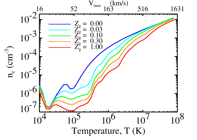
Figure 2: The cooling density as a function of halo temperature for several choices of gas metallicity. The cooling density increases dramatically with halo temperature. Thus massive halos can retain a larger fraction of their baryons in the form of hot gas then low mass halos.

3.3 The cooling radius

White & Frenk (1991) applied the concept of the cooling density as a function of radius in a dark matter halo, and introduced the concept of a cooling radius as a method to track the amount of cold gas available to form stars. This method has been adopted by most subsequent semi-analytic models of galaxy formation and seems to do an adequate job of reproducing the results of hydrodynamic simulations. The cooling radius, $R_{\rm c}$, is defined as the radius where the cooling density matches the initial hot gas density:

$$\rho_{\rm g}^{i}(R_{\rm c})\equiv\rho_{\rm c},$$ (16)

unless $\rho_{\rm c}<\rho_{\rm g}^{i}(R_{\rm v})$, in which case we will define $R_{\rm c}=R_{\rm v}$. For example, if the initial hot gas density follows that of a singular isothermal sphere then the cooling radius is

$$R_{\rm c}^{{}^{\rm SIS}}=\sqrt{{f_{b}V_{\rm max}^{2}}\over{4\pi G\rho_{\rm c}}}\simeq\,217\,{\rm kpc}\quad T_{{}_{6}}^{-1/2}(\Lambda_{z}t_{{}_{8}})^{1/2},$$ (17)

for $\rho_{\rm c}>\rho_{\rm g}^{i}(R_{\rm v})$.

While simple, the isothermal assumption is not a very good approximation for what we expect the initial hot gas profile to look like (Figure 4) and this can lead to large errors in the estimated size of $R_{\rm c}$ (see upper left panel of Figure 3). If instead we use our adopted initial gas profile (equation 9) then the value of $R_{\rm c}$ can be determined by solving a simple cubic equation. We find that an approximate fit to the solution for galaxy-size halos is

$$R_{\rm c}\simeq 157\,{\rm kpc}\,\quad T_{{}_{6}}^{-1/8}(\Lambda_{z}t_{{}_{8}})^{1/3}.$$ (18)

This expression is a good fit for the exact cooling radius solution for halos with $V_{\rm max}=\simeq 120-400{\rm km}\ {\rm s}^{-1}$, as shown by the dotted line in the upper-left panel of Figure 3 (see below). For $V_{\rm max}\lower 2.58334pt\vbox{\hbox{$\buildrel\textstyle<\over{\sim}\ $}}120{\rm km}\ {\rm s}^{-1}$, the virial radius will be the relevant outer radius (long dash line in Fig. 3):

$$R_{\rm v}\simeq 253\,{\rm kpc}\,\quad T_{{}_{6}}^{0.55}.$$ (19)

The above expressions are valid for $z=0$ in our cosmology.

Figure 3 shows the exact solution to equations 12 and 16 for various assumptions for the initial hot gas profile, halo formation time, redshift, and gas metallicity (clockwise from upper left) as a function of halo $V_{\rm max}$. The solid line in each panel shows the derived cooling radius for our fiducial set of assumptions, and the long-dashed line in each panel shows the halo virial radius. As seen in the bottom left panel, gas metallicity is important in setting the cooling radius because metal rich gas can cool more efficiently (and therefore at lower density and larger radius) than metal poor gas (see Fig 2). Note in the upper left panel that there is a large difference between assuming an SIS initial gas profile (short dash) and our NFW-inspired assumption (solid). Not only do NFW halos fall off more quickly in density at large radius, but they have smaller virial radii for a fixed $V_{\rm max}$.

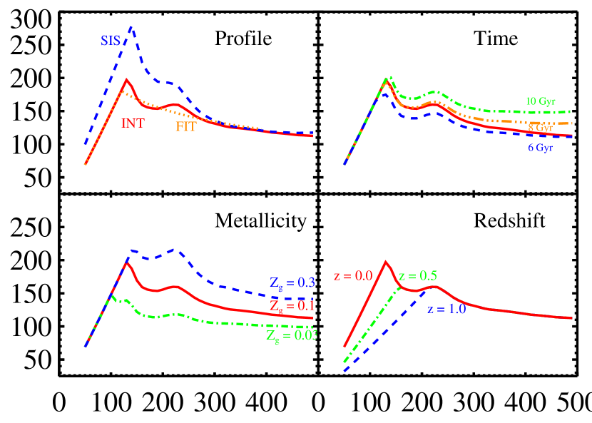
Figure 3: Cooling radius, $R_{\rm c}$, as a function of halo $V_{\rm max}$. In all panels, the solid line is $R_{\rm c}$ calculated with our fiducial choices of initial hot profile (equation 9), metallicity ($Z_{g}=0.1$) and formation time (equation 8) at $z=0$ as a function of halo $V_{\rm max}$ (assuming an NFW halo). Upper Left: Dependence of $R_{\rm c}$ on the initial hot gas profile. The short-dashed line assumes an SIS gas distribution and halo profile. The “INT” label refers to our initial hot gas profile, and the dotted line is our power-law approximation to this result (equation 18). Note that an SIS halo has a larger virial radius at fixed $V_{\rm max}$. Upper Right: Dependence of $R_{\rm c}$ on formation time. Lower Right: Dependence of $R_{\rm c}$ on redshift, for a fixed formation time (changing only the $V_{\rm max}$ to $R_{\rm v}$ relation). Lower Left: Dependence of $R_{\rm c}$ on metallicity.

4 A two-phase model of cooling

In the standard prescription, the evolution of $R_{\rm c}$ with time is used to evaluate the amount of gas available to form stars. All of the gas within the $R_{\rm c}$ sphere cools into the central galaxy (over the halo formation time). The gas outside of this sphere is assumed to stay there, at the virial temperature of the halo, tracing the background dark halo profile. As time goes on, the cooling radius grows, and so does the supply of cold, star-forming gas. In essence, $R_{\rm c}$ is used as a book-keeping tool, since clearly this shell-like structure of hot gas represents an unphysical, hydro-dynamically unstable configuration (at least if $R_{\rm c}<R_{\rm v}$). The physical situation this approximation most closely mirrors is one in which all of the gas within the cooling radius cools and contracts monolithically over the cooling time, with hot gas from the outer regions moving in as a result. The implicit assumption is that the thermal instability inherent in the gas is unimportant in governing the gas infall within the cooling radius.

A different, perhaps more physically-motivated picture arises by considering the two-phase nature of the gas. As mentioned, gas within $R_{\rm c}$ is subject to the thermal instability, and will tend to cool via cloud fragmentation. That is, not all of the gas within $R_{\rm c}$ will cool, but rather a two-phase (warm/hot) medium will develop. Warm ($\sim 10^{4}$K) clouds will form and grow until the background density of hot gas is reduced to roughly $\rho_{\rm c}$. Thus there is always a core of hot gas that extends to the center of the halo and that can provide pressure support for the hot gas outside of $R_{\rm c}$.

4.1 Cloud Formation and the Thermal Instability

Field (1965) first studied the thermal stability of astrophysical gases, which was extended to non-equilibrium systems by Balbus (1986). In the equilibrium case with no heating the instability criteria is

$$\left|{{\partial\ln{\Lambda}}\over{\partial\ln{T}}}\right|_{P}<1.$$ (20)

Using the fitting formula described in Appendix A (equation A), we see that hot gas should be unstable in all galaxy-size systems. Specifically, gas will tend to fragment in halos with temperatures above the metal-line cooling temperature $T_{m}\simeq 1.5\times 10^{5}$K. The range of instability extends below $T_{m}$ if the gas metallicity is less than solar.

The thermal instability leads to the rapid growth of perturbations and to the formation of warm gas fragments within the hot gas background (see §5.1 and also Murray & Lin, 1990). Perturbations can be either in the gas temperature or density and may be seeded by the accretion of substructure into the galaxy’s halo. Most of the perturbing halos will have virial temperatures much below $10^{4}$K and therefore will not gravitationally bind the clouds that form. Of course, some of the most massive subhalos may drive perturbations to become gravitationally bound to them; however, as we will be focusing on a scenario with an order of magnitude more clouds than massive dark matter substructures, we will assume that this is not the case for most of the clouds. For a treatment of warm clouds in dark matter substructure see Gnat & Sternberg (2004) and Sternberg et al. (2002).

The overdense, low-temperature regions that fragment will cool via atomic line cooling until they reach a temperature of $T_{\rm w}=10^{4}$ K and form clouds embedded within the hot, high-pressure background medium. Further cooling of the warm gas into cold ($\sim 300$K) material likely will be prevented because of the presence of the extragalactic ionizing background, at least for the typical cloud densities that we derive below.

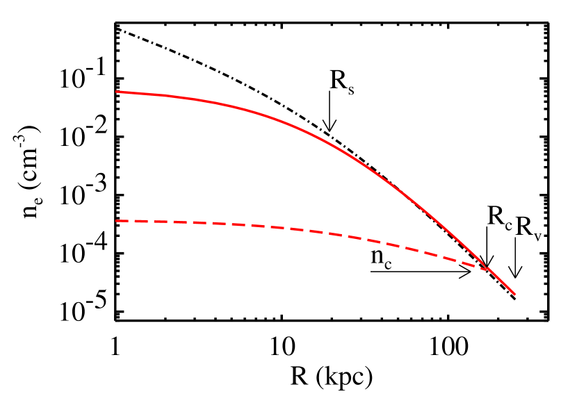
Figure 4: The solid line shows the initial gas profile given by equation 9 for a halo with $T=10^{6}$K ($V_{\rm max}=163{\rm km}\ {\rm s}^{-1}$). For comparison, an NFW profile (dot-dashed line) is shown normalized to the same total mass. The virial radius $R_{\rm v}$, the NFW scale radius $R_{\rm s}$, and the cooling radius $R_{\rm c}$ are also marked. In the standard cooling argument, all gas within the cooling radius contracts to form a central galaxy. In our two-phase model, there is a core of hot gas (dashed line) that extends to the center of the halo providing pressure support for the gas. In our scenario, the mass that cools is the integrated mass difference between the solid line and the dashed line.

4.2 Residual Hot Profile

After the clouds form out of the original hot gas halo, a residual hot gas component will be left. We can work out a model for this distribution by assuming that the gas returns to hydrostatic equilibrium within the gravitational potential of its dark matter halo. If the residual hot gas does not radiate significantly then it will adjust to the pressure change adiabatically. This is roughly what is seen in the cores of the clusters simulated Frenk et al. (1999) using non-radiative codes (note especially the high-resolution result of Bryant’s code). Thus we assume that the gas is adiabatic within $R_{\rm c}$, with $P\propto\rho_{h}^{5/3}$ (as adopted by Mo & Miralda-Escude, 1996). Of course, it would be useful to test this assumption with more detailed multi-phase cooling simulations in the future.

If we normalize by demanding that the hot gas reaches the cooling density at the cooling radius, and assume an NFW gravitational potential (neglecting the contribution of the baryons) then we find that the temperature and density profiles of the residual hot gas halo follow (see Appendix B)

$$\rho_{\rm h}(x) = \rho_{c}\left[1+\frac{3.7}{x}\ln(1+x)-\frac{3.7}{C_{\rm c}}\ln(1+C_{\rm c})\right]^{3/2}$$ (21)

$$T_{\rm h}(x) = T\left[1+\frac{3.7}{x}\ln(1+x)-\frac{3.7}{C_{\rm c}}\ln(1+C_{\rm c})\right],$$

where the radius $R$ is expressed as $x\equiv R/R_{\rm s}$ and $C_{\rm c}\equiv R_{\rm c}/R_{\rm s}$. We have assumed that the hot gas temperature at $R_{\rm c}$ is equal to the halo temperature $T$, defined with respect to $V_{\rm max}$ in equation 5. If $R_{\rm c}<R_{\rm v}$, we assume that the profile outside of $R_{\rm c}$ is isothermal. This solution is plotted for a halo with $V_{\rm max}=163{\rm km}\ {\rm s}^{-1}$ in Figure 4. The presence of a hot gas core implies that at least some fraction of the gas within the cooling radius remains hot.

For simplicity in the calculations that follow, we work under the approximation that the temperature, density, and pressure of the hot gas can be treated as constants as a function of radius within $R_{\rm c}$. As can be seen in Figure 4, this is certainly a reasonable approximation for the density. In Appendix B we show that the volume-averaged temperature, density, and pressure of the hot gas within the cooling radius for expression (21) are given by

$$\bar{T_{h}}=\eta_{T}T,\quad\bar{\rho_{h}}=\eta_{\rm d}\rho_{c},\quad\bar{P_{h}}=\eta_{P}P_{c},$$ (22)

with $\eta_{T}\simeq 1.0,$ $\eta_{\rm d}\simeq 1.35$, and $\eta_{P}\simeq 2.7$. We adopt these values in our treatment below.

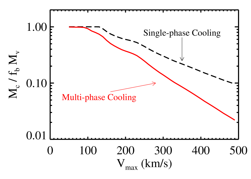
Figure 5: The fraction of baryons in the halo that cool as a function of halo maximum circular velocity in our model (solid line). This fraction quickly falls from $\sim 90\%$ at $100\,{\rm km}\ {\rm s}^{-1}$ to $\sim 2\%$ at $500\,{\rm km}\ {\rm s}^{-1}$. Also shown is the same quantity computed using the standard, single phase cooling scenario (dashed line). The difference arises from the additional hot gas core that develops in the multi-phase treatment.

4.3 Cooling Efficiency

Interestingly, including the simple expectation of a hot gas core changes the cooled-gas fraction in galaxy-size halos appreciably compared to the standard estimate. In the standard model, all of the gas inside of the cooling radius is assumed to cool. For the initial gas profile given in equation 9 this mass is

$$M_{R_{\rm c}}\equiv M_{g}^{i}(<R_{\rm c})=M_{b}\frac{g(C_{\rm c})}{g(C_{\rm v})},$$ (23)

where $M_{b}=f_{b}M_{\rm v}$. In our picture, $M_{R_{\rm c}}$ is divided between cooled gas and the hot gas corona. The total mass in cooled material, $M_{\rm c}$, is always less than $M_{R_{\rm c}}$ because of the presence of a hot core of mass $M_{\rm h}$:

$$M_{\rm c}=M_{R_{\rm c}}-M_{\rm h},\quad M_{\rm h}=\frac{4}{3}\pi\bar{\rho_{\rm h}}R_{\rm c}^{3}.$$ (24)

Here $\bar{\rho_{h}}\propto\rho_{\rm c}$ is the average density of the residual hot gas profile within $R_{\rm c}$.

The difference is illustrated explicitly in Figure 5. Shown is the fraction of baryons that have cooled in the halo for both the single phase (dashed) and multi-phase cooling (solid) as a function of halo $V_{\rm max}$. For galaxy-size halos, the multi-phase treatment reduces the cold gas fraction by $\sim 40\%$ compared to the standard case. This difference will be amplified if some fraction of the the gas that cools persists in the halo as warm clouds (see § 6). The effect of the hot core is more important for high-mass halos because the cooling density increases with temperature (see Fig. 2). For $V_{\rm max}\simeq 500{\rm km}\ {\rm s}^{-1}$ systems, the total amount of cooled gas is reduced by a factor of $\sim 5$ compared to the standard treatment. As discussed in §9, this may have important implications for understanding the bright cutoff in the galaxy luminosity function.

4.4 Cloud Size and Density

For cloud masses of interest, self-gravity will not be important in setting cloud sizes (see §5.6). Instead, pressure-confinement will set a typical cloud pressure and density. The implied density of a cloud is

$${\rho}_{w}=\rho_{\rm c}\frac{\eta_{P}T}{T_{\rm w}},$$ (25)

where $T_{\rm w}$ is the temperature of the warm cloud. We assume that the clouds are roughly constant density, so that a cloud of mass $m_{\rm cl}$ will have a characteristic radius

$$r_{\rm cl}=\left[{{3m_{\rm cl}}\over{4\pi{\rho}_{w}}}\right]^{1/3}\simeq 0.8{\rm kpc}\quad m_{6}^{1/3}T_{{}_{6}}^{-1}(\Lambda_{z}t_{{}_{8}})^{1/3},$$ (26)

where $m_{6}=m_{\rm cl}/10^{6}M_{\odot}$, and we have used $\eta_{P}=2.7$ and $T_{\rm w}=10^{4}K$.

At this stage, the cloud mass is the primary unknown parameter. We have normalized our cloud size using a characteristic mass $m_{\rm cl}=10^{6}M_{\odot}$, and we argue below that this may be an suitable mass for a variety of reasons. Modeling the underlying mechanisms that determine cloud masses is beyond the scope of the current work. We will instead attempt to constrain the allowed parameter space of clouds using both theoretical limits and, later, observational hints. Specifically, in the next section we consider various processes in the halo that will act to destroy clouds, and use these to set limits on viable cloud masses.

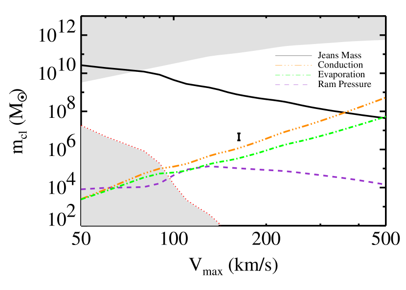
Figure 6: Properties of warm clouds as a function of $V_{\rm max}$. The upper shaded region shows the total mass within $R_{\rm c}$ as a function of the halo’s maximum circular velocity. Clearly the cloud mass must be less than this. The solid line shows the Jeans mass of the cloud. The triple-dot-dashed line shows the minimum mass cloud that can form in the presence of conduction with $f_{s}=0.2$ (see §5.2). Masses above the dot-dashed will survive conductive evaporation over a time $t_{f}$ (again taking $f_{s}=0.2$). For masses below the short-dashed line, ram pressure drag will cause clouds to move more slowly than the halo velocity, making them unlikely candidates for High Velocity Clouds. The shaded region in the lower left shows where clouds will be destroyed by Kelvin-Helmholtz instability by having a cooling time longer than the cloud sound crossing time. The error bar shows the cloud masses of interest for Milky-Way size halos ($V_{\rm max}=163{\rm km}\ {\rm s}^{-1}$) which help explain HVCs, high-ion absorption systems and the Milky-Way galaxy mass within our picture (see §7, §8, and §6.2 respectively).

5 Cloud masses

The physical processes that can act to limit the masses of warm clouds include conduction, evaporation, the Kelvin-Helmholtz instability, and the speed at which clouds can cool. Except for the last case, these processes impose a lower-mass limit on clouds that can survive. If the initial fluctuation distribution is power-law, it is perhaps reasonable to assume that clouds will tend to inhabit the lowest-mass regime allowed (Lin & Murray, 1992). Another interesting mass is the Jeans mass, which does not necessarily affect cloud survival, but may determine the mass scale above which star formation becomes efficient. Similarly, the relative importance of pressure drag on a cloud compared to the gravitational force will vary as a function of mass and this will set a lower limit on mass scales of interest for HVCs.

The discussion that follows is somewhat lengthy, and we provide a summary now, in conjunction with Figure 6, aimed at the reader who wishes to move beyond this section to the results. Figure 6 shows a space of cloud masses $m_{\rm cl}$ versus halo $V_{\rm max}$. In order to guide the eye, we have placed an error bar on the figure to illustrate the cloud masses of interest for Milky-Way size halos ($V_{\rm max}=163{\rm km}\ {\rm s}^{-1}$) which help explain HVCs, high-ion absorption systems and the Milky-Way galaxy mass within our picture (see §7, §8, and §6.2 respectively). The upper shaded region is excluded on physical grounds, as masses above its lower edge exceed the total baryonic mass within the halo’s cooling radius, $M_{R_{\rm c}}$. The shaded region in the lower left corner, below the dotted line, is excluded because clouds in this mass-velocity regime will be destroyed by Kelvin-Helmholtz instabilities (§5.3). The triple-dot-dashed line that runs just below the error bar is the characteristic cloud mass that arises if conduction sets the cloud fragmentation scale in the initial hot gas halo (§5.2). The dot-dashed line shows the minimum cloud mass that could have survived evaporation within the hot gas halo (§5.4). The solid line is the dividing line between Jeans stable (below) and unstable clouds (§5.6). Finally, the dashed line shows the mass below which ram pressure drag will cause clouds to move at speeds below $\sim V_{\rm max}$, and thus be unlikely candidates for HVCs (§5.5). The main conclusion here is that the cloud masses of observational interest are viable based on these considerations.

The analytic expressions that follow were calculated assuming the cooling curve power-law in equation 13, and therefore are valid only for galaxy-size halos ($V_{\rm max}\simeq 60-300{\rm km}\ {\rm s}^{-1}$). The lines in Figure 6 were determined using the $Z_{g}=0.1$ cooling curve shown in Figure 1.

5.1 Cloud Formation: The Ability to Fragment

As a result of the cooling instability discussed in §4.1, the contrast between temperature or density fluctuations in the initial hot halo will begin to grow as cooling proceeds. As slightly cooler regions begin to cool, they get denser and in turn, cool even more quickly, and this can lead to cloud formation. Specifically, if the over-cool region compresses more quickly than the background medium can cool, a separate warm cloud will form within the hot gas background. Burkert & Lin (2000) studied this process in some detail, and showed that warm, dense fragments will emerge in the hot medium as long as the density growth becomes nonlinear before the cooling becomes isochoric. The condition for cloud formation is that the sound-crossing time, $\tau_{\lambda}\simeq\lambda_{i}/c_{\rm h}$, along a perturbation of wavelength $\lambda_{i}$, should be less than the characteristic cooling time for the halo, which by our definition of the cooling density equals $t_{f}$. Here we have introduced $c_{\rm h}=V_{\rm max}/\sqrt{2}$ as the sound speed of the hot gas. Let us write the eventual cloud mass in terms of the initial fluctuation size as $m_{\rm cl}=4\pi(\lambda_{i}/2)^{3}\rho_{c}/3$. The condition $\tau_{\lambda}<t_{f}$ sets an upper limit on the cloud masses that will form

$$m_{\rm cl}\,\lower 2.58334pt\vbox{\hbox{$\buildrel\textstyle<\over{\sim}\ $}}8.4\times 10^{11}M_{\odot}T_{{}_{6}}^{7/3}\Lambda_{z}^{-1}t_{{}_{8}}^{2}.$$ (27)

We conclude that all mass scales of interest should be able to form clouds before isochoric cooling occurs. Indeed, this upper limit generally exceeds the total baryonic mass available within halos.

5.2 Cloud Formation: The Conduction Limit

A more interesting limit arises from considering conduction. If conduction is important in the hot gas halo, this can dampen temperature fluctuations and inhibit the formation of clouds. The length scale below which conduction will be important compared to cooling (or heating) is known as the Field length (McKee & Begelman, 1990; Field, 1965)

$$\lambda_{F}=\left[\frac{T\kappa(T)}{n_{e}^{2}\Lambda(T)}\right]^{1/2},$$ (28)

where $\kappa$ is the conductivity of the gas. One can characterize the conductivity as a fraction $f_{s}<1$ of the classical Spitzer (1962) conductivity:

$$\kappa\equiv f_{s}\kappa_{\rm sp}=f_{s}{{1.84\times 10^{10}T_{{}_{6}}^{5/2}\over\ln\Lambda_{\rm C}}}{\rm erg}\,\rm{cm}^{-1}\,\rm{s}^{-1}\,K^{-1},$$ (29)

where $\ln\Lambda_{\rm C}$ is the Coulomb logarithm, and we adopt $\ln\Lambda_{\rm C}=35$ as an appropriate value for the temperature and density range of interest (Cowie & McKee, 1977). For an unmagnetized plasma, $f_{s}$ is unity and conduction is efficient. The presence of magnetic fields can make $f_{s}$ quite small, with $\sim 0.001$ if the fields are uniform or moderately tangled (Chandran & Cowley, 1998). However Narayan & Medvedev (2001) have shown that $f_{s}\sim 0.1$ in a medium where magnetic fields are chaotic over a wide range of length scales. The results of Zakamska & Narayan (2003) imply that $f_{s}\simeq 0.2$ can help solve the cooling flow problem in clusters (see also Kim & Narayan, 2003). We will adopt $f_{s}=0.2$ as our fiducial value here. With this choice we find that the Field length of a hot gas at the cooling density is

$$\lambda_{F}\simeq 11{\rm kpc}\quad T_{{}_{6}}^{1/4}\Lambda_{z}^{1/2}t_{{}_{8}}f_{0.2}^{1/2}.$$ (30)

Scales smaller than $\lambda_{F}$ will tend to have a uniform temperature, and this implies a characteristic lower-limit on the mass: $m_{cl}^{\rm F}\equiv 4\pi(\lambda_{F}/2)^{3}\rho_{c}/3$. Using typical numbers we find

$$m_{cl}^{\rm F}\simeq 1.2\times 10^{6}M_{\odot}\quad T_{{}_{6}}^{11/4}\Lambda_{z}^{1/2}t_{{}_{8}}^{2}f_{0.2}^{3/2}.$$ (31)

We plot the Field mass as a function of $V_{\rm max}$ for $f_{s}=0.2$ as the triple-dot-dashed line in Figure 6. Note that $m_{cl}^{\rm F}$ as defined above scales as $f_{s}^{3/2}$. If conduction operates at $\sim 20\%$ the Spitzer value, the characteristic mass scale is quite similar to our mass scale of interest.

We point out that if $\lambda_{F}\lower 2.58334pt\vbox{\hbox{$\buildrel\textstyle>\over{\sim}\ $}}R_{\rm c}$, we expect cloud fragmentation to be stabilized completely. When this occurs, conductive heating from outside of $R_{\rm c}$ can play an important role in setting the temperature structure of halos. This occurs when $T\lower 2.58334pt\vbox{\hbox{$\buildrel\textstyle>\over{\sim}\ $}}3.2\times 10^{7}K$ ($V_{\rm max}\lower 2.58334pt\vbox{\hbox{$\buildrel\textstyle>\over{\sim}\ $}}920{\rm km}\ {\rm s}^{-1}$), or in massive cluster-size systems. (Note that the scaling in equation 31 is only valid for $60{\rm km}\ {\rm s}^{-1}\lower 2.58334pt\vbox{\hbox{$\buildrel\textstyle<\over{\sim}\ $}}V_{\rm max}\lower 2.58334pt\vbox{\hbox{$\buildrel\textstyle<\over{\sim}\ $}}300{\rm km}\ {\rm s}^{-1}$ because we have assumed a power-law form for the cooling function in its derivation.)

5.3 Cloud Survival: The Kelvin-Helmholtz Instability

Once clouds form they are subject to shearing stresses across their boundary as they travel through the hot medium. The flow can be subject to perturbations, and this is characterized as the Kelvin-Helmholtz instability (KHI).

The dominate destructive process is the “champagne effect”, which results from the development of a low-pressure, fast flow around the head of the moving cloud (Doroshkevich & Zeldovich, 1981; Murray et al., 1993; Vietri et al., 1997). By Bernoulli’s theorem, the pressure exerted by the fast wind at the head of the cloud is low, so the cloud’s inner pressure can cause its material to be pushed out from the top. Vietri et al. (1997) showed that the champagne effect is stabilized if the cooling time of a cloud is shorter than the sound crossing time of the cloud. That is, if the pressure waves inside the cloud are damped by radiative cooling before they can cross the cloud, then the inner part of the cloud cannot respond to produce the over-spilling. Note that this result holds even for clouds that are in thermal equilibrium with a background field, as assumed here.

Based on the work of Vietri et al. (1997), we would like to compare the cooling time of our clouds to the sound crossing time. This will determine if they are stable against the KHI. The sound crossing time of the cloud is $\tau_{\lambda}^{\rm cl}=r_{\rm cl}/c_{\rm w}$, where $c_{\rm w}\simeq 11.5{\rm km}\ {\rm s}^{-1}$ is the speed of sound in the warm medium. Using equation 26 for the cloud size we obtain

$$\tau_{\lambda}^{\rm cl}\simeq 6.7\times 10^{7}{\rm yrs}\quad m_{6}^{1/3}T_{{}_{6}}^{-1}(\Lambda_{z}t_{{}_{8}})^{1/3}.$$ (32)

We compare this to the the cooling time of a cloud of temperature $T_{\rm w}$ and density ${\rho}_{w}$:

$$\tau_{\rm c}^{\rm cl}=\frac{3\mu_{e}^{2}m_{p}k_{b}T_{\rm w}}{2\mu_{i}{\rho}_{w}\Lambda(T_{\rm w})}\simeq 1.6\times 10^{6}{\rm yrs}\quad T_{{}_{6}}^{-3}\Lambda_{z}t_{{}_{8}},$$ (33)

where we have used $\Lambda(T_{w}=10^{4}K)=4.9\times 10^{-24}{\rm cm}^{3}{\rm erg}\,{\rm s}^{-1}$ (see Figure 1). This allows us to define a characteristic KHI mass, above which clouds will be stable. By setting $\tau_{r_{\rm cl}}(m_{\rm cl})=\tau_{\rm c}$ we obtain

$$m_{\rm cl}^{\rm KHI}\simeq 10.5M_{\odot}\quad T_{{}_{6}}^{-6}(\Lambda_{z}t_{{}_{8}})^{2},$$ (34)

and note that the mass above which clouds are stable is a very strong function of the hot gas temperature. This is seen clearly by the shaded region in the lower left of Figure 6. As the host halo’s temperature goes down, clouds become less dense (see equation 25), their cooling times increase, and they are more susceptible to the KHI. We see that cooling alone stabilizes most cloud masses of interest except in low-temperature halos.

5.4 Cloud Survival: Conductive Evaporation

Clouds may also be evaporated by conduction from the surrounding hot gas. The characteristic evaporation time scale is given by

$$\tau_{\rm evap} = {{25k_{b}m_{\rm cl}}\over{16\pi\mu_{i}m_{p}\kappa(T)r_{\rm cl}}}$$

$$\simeq 16{\rm Gyr}\quad m_{6}^{2/3}T_{{}_{6}}^{-3/2}(\Lambda_{z}t_{{}_{8}})^{-1/3},$$

(Cowie & McKee, 1977) where we have taken $f_{s}=0.2$. If we set this equal to the halo formation time (i.e. if require that clouds forming at $t_{f}$ have not evaporated by today) this gives us a lower bound on the cloud mass of

$$m_{\rm cl}^{\rm Evap} = \sqrt{{3\pi^{2}}\over{{4{\rho}_{w}}}}\left[{{16\mu_{i}m_{p}\kappa(T)t_{f}}\over{25k_{b}}}\right]^{3/2}$$

$$\simeq 3.5\times 10^{5}M_{\odot}\quad T_{{}_{6}}^{9/4}\Lambda_{z}^{1/2}t_{{}_{8}}^{2}.$$

This is shown as the dot-dashed line in Fig. 6. Cloud masses above this line will not evaporate over a time $t_{f}$.

5.5 Cloud Motion: Ambient Drag

As the cloud moves through the hot gas halo at speed $\rm v_{cl}$, it will experience a “ram pressure” drag force that opposes its motion (e.g. Landau & Lifshitz, 1959)

$$F_{\rm ram}=\frac{1}{2}C_{\rm d}\bar{\rho_{h}}\rm v_{cl}^{2}\pi r_{\rm cl}^{2},$$ (37)

where $C_{\rm d}$ is the drag coefficient. Clouds reach terminal velocity, $v_{\rm t}$, when the gravitation force on the cloud is balanced by ram pressure force:

$$v_{\rm t}^{2}=2{{GM(D)m_{\rm cl}}\over{D^{2}\pi r_{\rm cl}^{2}\bar{\rho_{h}}C_{\rm d}}}=V_{\rm max}^{2}\left[\frac{8r_{\rm cl}\rho_{w}}{3DC_{\rm d}\bar{\rho_{h}}}\right].$$ (38)

For simplicity, we have assumed that the host halo is an isothermal sphere, with $D$ the distance from the cloud to the halo center. If we assume that a typical distance is $D\simeq R_{\rm c}$ then we obtain:

$${{v_{\rm t}}\over{V_{\rm max}}}=\sqrt{{8r_{\rm cl}\eta_{P}T}\over{3C_{\rm d}R_{\rm c}\eta_{\rm d}T_{\rm w}}}\simeq 1.6\quad m_{6}^{1/6}T_{{}_{6}}^{1/16}(\Lambda_{z}t_{{}_{8}})^{-1/12},$$ (39)

where we have used $\eta_{\rm d}=1.35$ and $C_{\rm d}=1.0$. Thus if clouds are sufficiently massive they can travel at a typical speed $\rm v_{cl}\simeq V_{\rm max}$ and not experience significant deceleration over a dynamical time. The limiting mass, below which $\rm v_{cl}<V_{\rm max}$ is

$$m_{\rm cl}^{\rm ram}\simeq 5.1\times 10^{4}M_{\odot}\quad T_{{}_{6}}^{-3/8}(\Lambda_{z}t_{{}_{8}})^{1/2}.$$ (40)

This mass scale is plotted as the dashed line in Figure 6. Clouds very much smaller than this are physically viable, but their slow speeds would make them unlikely candidates for “high-velocity” clouds. We return to the effect that ram pressure drag will have on cloud motion in §6.1.

5.6 Cloud Self-Gravity: Jeans Mass

The Jeans mass estimates when a fluid is unstable to self gravity. For a cloud confined by a pressure $P_{h}$ it is given by (Spitzer, 1978)

$$M_{J}={{9c_{\rm w}^{4}}\over{5G^{3/2}P_{h}^{1/2}}}.$$ (41)

Warm clouds with temperature $T_{\rm w}=10^{4}$ K have a sound speed $c_{\rm w}=11.5{\rm km}\ {\rm s}^{-1}$, and the minimum cloud mass that is unstable to self gravity is

$$m_{\rm cl}^{J}\simeq 7.2\times 10^{8}M_{\odot}\quad T_{{}_{6}}^{11/4}(\Lambda_{z}t_{{}_{8}})^{1/2}.$$ (42)

The Jeans mass for a warm cloud as a function of halo maximum circular velocity is plotted as the solid line in Fig. 6.

Our expectation is that clouds will be less massive than the Jeans mass in galaxy-size halos and therefore their self gravity can be ignored. However, it is possible that in high-mass halos that clouds will tend to be more massive. This might happen, e.g., if conduction sets the cloud mass (equation 31 and the triple-dot-dashed line in Fig. 6). In this case, the clouds may be above the Jeans mass, self-gravitating, and perhaps form stars in cluster-size halos. These objects would likely be spheroidal systems, with rather low mass-to-light ratios. Cluster “galaxies” of this type would not contain dark matter.

6 Galaxy Formation via cloud infall

The warm clouds are accelerated towards the center of the halo, but we do not expect that they will settle there immediately. Rather, clouds should have some distribution of energy and angular momentum that will have to be lost before the clouds merge with the central galaxy. For example, clouds may take on an angular momentum distribution similar to that of bulk-averaged regions seen in dark matter halo N-body simulations (Bullock et al., 2001) or of streaming motions in hydrodynamic simulations (van den Bosch et al., 2003). Clouds stripped from merging halos are expected to have a similar distribution (Maller & Dekel, 2002).

For concreteness, we will assume that the clouds take on an energy distribution with a characteristic velocity equal to the halo velocity, $\rm v_{cl}=V_{\rm max}$. Cloud-cloud collisions or ram pressure drag eventually lead to cloud orbital decay. In our picture, it is this cloud infall that sets the gas supply that governs the formation of the central galaxy. In the following subsections, we discuss expected infall times, explore the implied central galaxy mass and residual cloud population, and discuss the disruption of clouds as they approach the galaxy.

6.1 Infall Times

As clouds orbit within the hot gas halo they will experience ram pressure drag (equation 37). The continuous drag will sap energy from the clouds, and this can eventually lead to orbital decay. The timescale for this to occur is given by

$$\tau_{\rm ram}={{2m_{\rm cl}}\over{\pi C_{\rm d}r_{\rm cl}^{2}\bar{\rho_{h}}\rm v_{cl}}}\simeq 2.6{\rm Gyr}\quad m_{6}^{1/3}T_{{}_{6}}^{-1/2}(\Lambda_{z}t_{{}_{8}})^{1/3},$$ (43)

if $\rm v_{cl}=V_{\rm max}$ and $C_{\rm d}=1$. Thus for $10^{6}M_{\odot}$ clouds, only those that cooled out of the hot gas more than $\sim 3$Gyr ago would have begun to sink to the center of the halo via ram pressure effects. If the drag coefficient, $C_{\rm d}$ is less than $1$, then this is a lower limit on the drag decay time. We show below that the mass in clouds that we expect to have fallen in or formed in the halo since that time may be a rather large fraction of the baryonic content of the Galaxy.

Cloud collisions will also be important in triggering cloud infall. We will assume, for simplicity, that after a collision, most of the cloud energy goes into heating the cloud material, and that this is quickly radiated away. The remaining, likely merged, system will have low kinetic energy and will quickly fall in to contribute to the central galaxy. Thus the cloud infall time will scale like the cloud-cloud collision time.

The mean free time between cloud collisions can be written as $\tau_{cc}\simeq(\phi_{\rm cl}\rm v_{cl}\sigma_{\rm cl})^{-1}$, where the cloud cross section is $\sigma_{\rm cl}\simeq\pi r_{\rm cl}^{2}$ and $\phi_{\rm cl}$ is the number density of clouds. Note that $\phi_{\rm cl}$ depends on the total mass of warm clouds $M_{\rm cl}$, and that this will change as clouds collide and merge or if new clouds form. If we assign $\phi_{\rm cl}=3M_{\rm cl}/(m_{\rm cl}4\pi R_{\rm c}^{3})$ we can write the cloud-cloud collision time as

$$\tau_{cc}={{4m_{\rm cl}R_{\rm c}^{3}}\over{3M_{\rm cl}\rm v_{cl}r_{\rm cl}^{2}}}\simeq 2.4{\rm Gyr}\quad\quad m_{6}^{1/3}T_{{}_{6}}^{9/8}(\Lambda_{z}t_{{}_{8}})^{5/6}M_{2.10}^{-1}.$$ (44)

Here we have used $M_{2.10}\equiv M_{\rm cl}/(2\times 10^{10}M_{\odot})$ as the characteristic mass in clouds that we expect to exist in our fiducial halo. We explain this expectation in more detail in §6.2. We stress, however, that $M_{\rm cl}$ should vary as a function of halo mass and cloud mass, so their are additional dependencies in equation 44 that are hidden in this variable.

When the density of clouds is high, $\tau_{cc}$ is small, and clouds will quickly collide and sink to the center. As the total number of clouds drops, the cloud infall rate will begin to drop as well. It is useful to consider the simple scenario where we start with a number density of clouds $\phi_{0}$ in a fixed volume. In this case the number density of clouds as a function of time obeys $d\phi/dt=\phi(t)\tau^{-1}=\phi^{2}(\tau_{0}\phi_{0})^{-1}$, where $\tau_{0}$ is the mean free time initially. The solution is $\phi(t)=\phi_{0}/(1+t/\tau_{0})$, so there will always be a residual cloud population in any halo, if cloud collisions set the infall rate.

We mention that the shortest timescale over which clouds can fall in to the central galaxy is the free-fall time, $\tau_{\rm ff}$. If we estimate the cloud free-fall time from the cooling radius as $\tau_{\rm ff}=R_{\rm c}/V_{\rm max}$ then we obtain

$$\tau_{\rm ff}\simeq 0.94{\rm Gyr}\quad T_{{}_{6}}^{-5/8}(\Lambda_{z}t_{{}_{8}})^{1/3}.$$ (45)

This expression is accurate for halos with maximum circular velocities of $120{\rm km}\ {\rm s}^{-1}\lower 2.58334pt\vbox{\hbox{$\buildrel\textstyle<\over{\sim}\ $}}V_{\rm max}\lower 2.58334pt\vbox{\hbox{$\buildrel\textstyle<\over{\sim}\ $}}400{\rm km}\ {\rm s}^{-1}$ (where $R_{\rm c}<R_{\rm v}$ sets the lower limit and the breakdown in the scaling $\Lambda(T)\propto T^{-1}$ sets the upper limit). For all cases that we consider, the free-fall timescale is shorter than both $\tau_{cc}$ and $\tau_{\rm ram}$.

6.2 Central Galaxy Mass

The total mass within the halo cooling radius, $M_{R_{\rm c}}$, is divided between gas in the hot halo core, $M_{\rm h}$, and gas that has cooled since the halo formation time $M_{\rm c}$ (equation 24). The cooled gas mass is itself shared between warm clouds, $M_{\rm cl}$, and the central galaxy $M_{\rm g}$. The mass budget is then described by

$$M_{R_{\rm c}} = M_{\rm h}+M_{\rm c}$$ (46)

$$M_{\rm c} = M_{\rm cl}+M_{\rm g}.$$

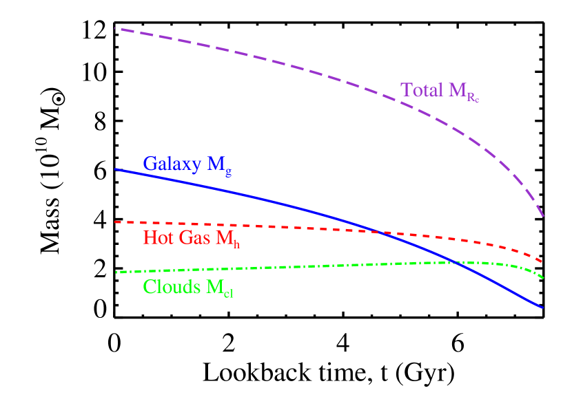
Figure 7: Evolution of each baryonic component as a function of lookback time. The long dashed line shows the the total baryonic mass within the cooling radius, which grows steadily as a function of time. The central galaxy mass (solid line) also grows with time, as clouds continue to fall in. The total mass in the hot gas core (short dashed line) remains roughly constant as the cooling radius grows and cooling density drops. The total mass in clouds (dot-dashed line) remains nearly constant, as cloud formation and infall are balanced.

We assume that cooling proceeds by the formation of clouds and that the infall of clouds leads to galaxy growth. The evolution of the total mass in clouds as a function of time can be modeled as a competition between cold mass accumulation (as the cooling radius grows) and the rate of cloud “destruction” via infall onto the galaxy:

$$\frac{dM_{\rm cl}}{dt} = \frac{dM_{\rm c}}{dt}-\frac{dM_{\rm g}}{dt}$$ (47)

$$\frac{dM_{\rm g}}{dt} = \frac{M_{\rm cl}}{\tau_{\rm in}}.$$

We have associated the cloud infall rate with the rate of galaxy growth, and set this equal to $M_{\rm cl}/\tau_{in}$. Here $\tau_{in}$ is a characteristic cloud infall time, chosen to be the minimum of $\tau_{cc}$ and $\tau_{\rm ram}$. For the fiducial halo and cloud mass discussed in this section, $\tau_{cc}<\tau_{\rm ram}$, and cloud-cloud collisions dominate the infall.

It is straightforward to solve this simple set of equations (46, 47) in order to evaluate the mass in each component. Once we choose a halo $V_{\rm max}$, the evolution of the hot gas core mass, $M_{\rm h}(t)$, is governed entirely by the evolution of the cooling radius and corresponding evolution in the cooling density (equations 14, 18, 24). The evolution of $M_{\rm c}$ with time can similarly be determined by the evolution of $R_{\rm c}(t)$ (equation 18) and $M_{\rm h}(t)$ (as just described). The other components may be tracked via equation 47 once one adopts a cloud mass, $m_{\rm cl}$, and evaluates $\tau_{\rm in}(t)$ using equation 44 or 43.

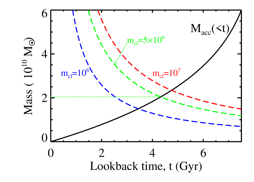
Figure 8: Shown as the solid line is the amount of mass that has cooled as a function of lookback time: $M_{\rm acc}(t)=M_{\rm c}(0)-M_{\rm c}(t)$. The dashed lines show the total mass in clouds that would have a collision time, $\tau_{cc}$, that is equal to the lookback time plotted on the x-axis. We show the result for three cloud masses, $(1,5,10)\times 10^{6}M_{\odot}$. The point where a dashed line intersects the solid line gives the approximate mass in clouds that can survive until $t=0$ (today). For a typical cloud mass $m_{\rm cl}=5\times 10^{6}M_{\odot}$, the expected residual mass in clouds is $M_{\rm cl}\simeq 2\times 10^{10}M_{\odot}$ (as indicated by the dotted line), which is in good agreement with what is found by integrating the set of equations discussed in the text and shown in Fig. 7.

Figure 7 shows the resulting buildup in each mass component as a function of lookback time for our fiducial “Milky Way” halo of $V_{\rm max}=163{\rm km}\ {\rm s}^{-1}$, and a cloud mass of $m_{\rm cl}=5\times 10^{6}M_{\odot}$. The top long-dash line shows the total baryonic mass within the cooling radius, $M_{R_{\rm c}}$, and the lower set of dot-dashed, short-dashed, and solid lines show the galactic mass, hot core mass, and total cloud mass ($M_{\rm g}$, $M_{\rm h}$, and $M_{\rm cl}$) respectively. The most striking result is that the final galaxy mass, $M_{\rm g}\simeq 6\times 10^{10}M_{\odot}$, is roughly half of the mass it would have been had we adopted the standard treatment, and allowed all of the mass within $R_{\rm c}$ to contribute, $M_{R_{\rm c}}\simeq 12\times 10^{10}M_{\odot}$. The mass in clouds peaks rather early at $M_{\rm cl}\simeq 2\times 10^{10}M_{\odot}$, and then remains relatively constant as the cloud infall rate is matched by the rate of accumulation of cooled gas. The mass within the hot core also remains relatively constant as a function of lookback time $M_{\rm h}\simeq 4\times 10^{10}M_{\odot}$. This is because $M_{\rm h}\propto n_{\rm c}R_{\rm c}^{3}$, and growth in $R_{\rm c}$ at late times is canceled out by the decrease in $n_{\rm c}$ (this can be seen via inspection of the time scalings in equations 14 and 18).

The final residual cloud mass expected in this scenario is straightforward to understand without having to solve the differential equations. Given a characteristic cloud infall time $\tau_{\rm in}$, we expect clouds to remain in the halo as long as $\tau_{\rm in}$ is longer than the time since the clouds were formed (or accreted).

Consider a case where $\tau_{\rm in}=\tau_{cc}$ and cloud-cloud collisions dominate infall. The solid line in Figure 8 shows the amount of mass that has cooled since a lookback time $t$. Specifically, $M_{\rm acc}(t)=M_{\rm c}(0)-M_{\rm c}(t)$. We have used the same $V_{\rm max}=163{\rm km}\ {\rm s}^{-1}$ halo discussed in conjunction with Figure 7. The three dashed lines in Figure 8 correspond to cloud-cloud collision times computed using three different cloud masses $m_{\rm cl}=(1$, $5$, and $10)\times 10^{6}M_{\odot}$. In each case we show the amount of mass needed in clouds to get a $\tau_{cc}$ equal to the time on the x-axis. Note that cloud-cloud collision times are short if the total mass in clouds is large. The point where the dashed lines cross the solid line corresponds to the mass in clouds that could have survived until the present day without merging into the galaxy. Thus, for the central line ($m_{\rm cl}=5\times 10^{6}M_{\odot}$) we expect a final mass in clouds of $M_{\rm cl}\simeq 2\times 10^{10}M_{\odot}$ to have survived until the present day. ¿From Figure 7 we see that this is very close to the mass in clouds derived from integrating equations (46 and 47). This simple method allows a quick way to estimate the final central galaxy mass: $M_{\rm g}(0)\simeq M_{\rm c}(0)-M_{\rm acc}(\tau)$.

We have applied this simple treatment in Figure 9 in order to estimate the range of cloud masses that may help explain the baryonic mass of the Milky Way. The shaded band shows the estimated range of Milky Way galaxy masses derived by Dehnen & Binney (1998). The solid line shows the final galaxy mass, $M_{\rm g}$, and the dashed line shows the residual total mass in clouds, $M_{\rm cl}$, as a function of the individual cloud mass, $m_{\rm cl}$. Note that the Milky Way mass is matched well for $m_{\rm cl}\simeq 4\times 10^{6}-10^{8}M_{\odot}$ without including any blow-out feedback. Note however, that even if cloud masses are small ($m_{\rm cl}\lower 2.58334pt\vbox{\hbox{$\buildrel\textstyle<\over{\sim}\ $}}10^{6}M_{\odot}$) and fall in quickly to assemble the Galaxy, explaining the mass of the Milky Way is much easier in this picture because of the substantial hot gas core. The kinks in the lines occur at the cloud mass below which ram pressure dominates cloud infall. Cloud-cloud collisions are more important for massive clouds. The dotted line shows how the mass in clouds would change had we set the cloud drag constant to zero, so that ram pressure was unimportant in cloud evolution.

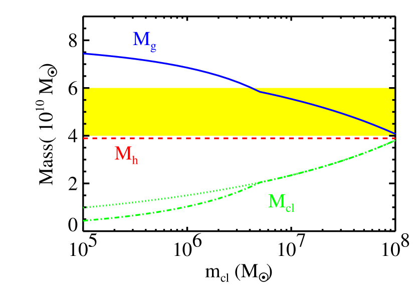
Figure 9: Shown is the mass in the hot gas core (dashed), mass in warm clouds, with and without ram pressure (dot-dashed and dotted) and mass in the galaxy (solid) as a function of the warm cloud mass. The shaded region shows the range of masses for the Milky Way (Dehnen & Binney, 1998). Cloud masses in the range $(4-100)\times 10^{6}M_{\odot}$ allow agreement with estimated Milky Way mass without including any blow-out feedback.

6.3 Tidal Disruption

As clouds approach the central galaxy they will experience strong tidal forces and may be destroyed. If clouds are broken up before impacting the galaxy, this will prevent them from causing too much heating or damaging the disk. Tidally deformed clouds will tend to be quite large, and perhaps can be identified with the large HI complexes that are well known to exist in proximity to the Milky Way (Tripp et al., 2003; Wakker & van Woerden, 1991; Blitz et al., 1999).

Clouds will be disrupted when the tidal force from the host potential overcomes the pressure confinement of the clouds. At a distance $D$ from the host center, assuming that the host potential is roughly isothermal, the tidal force felt across a cloud of radius $r_{\rm cl}\ll D$ is approximated as

$$F_{T}\simeq{{GM_{\rm dm}(D)m_{\rm cl}r_{\rm cl}}\over{D^{3}}}.$$ (48)

This can be compared to the typical pressure force

$$F_{P}\simeq\pi r_{\rm cl}^{2}\eta_{P}\rho_{\rm c}T.$$ (49)

The radius $R_{\rm d}$ where the two forces are equal defines the surface of a sphere of disruption for the clouds. For an SIS density distribution $M(R)=G^{-1}V_{\rm max}^{2}R$, the tidal sphere for destroying clouds can be derived analytically:

$$R_{\rm d}\simeq 13\rm{kpc}\quad m_{6}^{1/3}T_{{}_{6}}^{-1/2}(\Lambda_{z}t_{{}_{8}})^{1/3}.$$ (50)

In the galaxy mass regime ($100{\rm km}\ {\rm s}^{-1}<V_{\rm max}<350{\rm km}\ {\rm s}^{-1}$) the value of $R_{d}$ for a SIS and a NFW halo are very similar. We see that the sphere of disruption is larger than the size of the Milky Way’s disk. It is therefore unlikely that the disk will be heated significantly from impacting clouds. Interestingly, this distance would be consistent with distance limits for many of the large HVC complexes (e.g. van Woerden et al., 1999b, a; Wakker et al., 2001).

7 Residual clouds as HVCs

Seen in 21 cm HI emission, High Velocity Clouds (HVCs) have been studied for more than four decades (Muller et al., 1963). Interpreting the observed properties of HVCs in terms of physical parameters requires knowing the radial distance, $D$, from the Sun. This is the major observational unknown that has fueled the debate over their origin since their discovery.

Models for HVCs range from condensed “Galactic Fountain” gas at $D\simeq 5$kpc (Shapiro & Field, 1976; Bregman, 1980), to large, extra-galactic objects associated with the Local Group $D\simeq 1$Mpc (Verschuur, 1969; Arp, 1985; Blitz et al., 1999; Blitz, 2002; Sternberg et al., 2002; Maloney & Putman, 2003). In our picture, the HVCs are “circumgalactic”, within the cooling radius of the Galaxy, and bear resemblance to the $D\simeq 100$kpc population suggested by Oort (1966).  

We expect that most of the mass in each cloud is in the form of ionized hydrogen at a temperature $T\simeq 10^{4}K$. Clouds of this kind would have a velocity distribution full-width-half-max (FWHM) of $\Delta v\simeq 27{\rm km}\ {\rm s}^{-1}$. The line width distribution of Compact HVCs studied by de Heij et al. (2002) has a median FWHM of $\Delta v=25{\rm km}\ {\rm s}^{-1}$. The agreement with predicted and observed line widths is encouraging.

The recent HIPASS survey cataloged HVCs over the entire southern sky (Putman et al., 2002). They find that the radial velocity distribution of their clouds is narrow when plotted with respect to the Galactic Standard of Rest, with $\sigma_{r}=115{\rm km}\ {\rm s}^{-1}$ (it is $\sigma_{r}=185{\rm km}\ {\rm s}^{-1}$ for the Local Standard of Rest). It peaks near $\sim 0{\rm km}\ {\rm s}^{-1}$. As discussed in the introduction, completely disjoint dynamical models of the Milky Way lead us to choose a fiducial “Milky Way” dark halo with $V_{\rm max}=163{\rm km}\ {\rm s}^{-1}$, and therefore a velocity dispersion very close to the GSR distribution of HVCs: $\sigma_{r}\simeq V_{\rm max}/\sqrt{2}=115{\rm km}\ {\rm s}^{-1}$. Since the residual clouds in our scenario should roughly take on the dark halo’s velocity distribution, we expect them to match the observed HVC distribution quite well.

The HIPASS HVC population has a characteristic peak $HI$ column density of $N_{HI}\simeq 10^{19}{\rm cm^{-2}}$ and a characteristic angular size of $\theta\simeq 0.5$deg² (Putman et al., 2002). The expected hydrogen space density for an individual cloud in our model is

$$n_{H}=\frac{\rho_{w}f_{H}}{m_{p}}\simeq 1.4\times 10^{-2}\rm{cm}^{-2}\quad T_{{}_{6}}^{3}(\Lambda_{z}t_{{}_{8}})^{-1},$$ (51)

where we assume that the mass fraction in Hydrogen is $f_{H}=0.7$. The column density in $HI$ through a cloud can be estimated via $N_{HI}=2r_{\rm cl}n_{H}\epsilon_{HI}$, with $\epsilon_{HI}$ the fraction of neutral hydrogen. With $\epsilon_{HI}=0.1$ (Maloney & Putman, 2003) we obtain

$$N_{HI}\simeq 6.8\times 10^{18}\rm{cm}^{-2}\quad m_{6}^{1/3}T_{{}_{6}}^{2}(\Lambda_{z}t_{{}_{8}})^{-2/3}.$$ (52)

If we demand $N_{HI}=10^{19}\rm{cm}^{-2}$ for our typical cloud in order to match observations, this would imply $m_{\rm cl}\simeq 3\times 10^{6}M_{\odot}$.

The angular size of the cloud is related to the cloud radius by

$$\theta_{\rm cl}\simeq 10^{4}\left[{{r_{\rm cl}}\over{D}}\right]^{2}{\rm deg}^{2}$$ (53)

where $D$ is the distance to the cloud. If we set $D=R_{\rm c}$ (equation 18), then the typical cloud area on the sky will be

$$\theta_{\rm cl}\simeq 0.25\,{\rm deg}^{2}\quad m_{6}^{2/3}T_{{}_{6}}^{-7/4}.$$ (54)

In order to match a typical size of $\theta_{\rm cl}=0.5$deg² we will need $m_{\rm cl}\simeq 3\times 10^{6}M_{\odot}$, which is nicely in line with what we needed to match the column density above. Of course, the angular sizes observed correspond to $HI$ sizes, and one might expect the outer radius in neutral material to be somewhat smaller that the full cloud radius. In the models of Maloney & Putman (2003), $r_{HI}\simeq 0.7r_{\rm cl}$ for constant-density clouds similar to the type we consider here. If we adopt this assumption, then the coefficient in equation 54 would scale to $0.18$ deg², and push our preferred mass to $m_{\rm cl}\simeq 5\times 10^{6}M_{\odot}$.

Finally, there are roughly 2000 HVCs in the HIPASS sample covering the southern sky. If we double this, we can estimate that the full halo should contain $\sim 4000$ such clouds. The number of clouds we expect in the halo is simply $N_{\rm cl}\simeq M_{\rm cl}/m_{\rm cl}$. In the previous section, we assumed cloud masses of $m_{\rm cl}=5\times 10^{6}M_{\odot}$ and computed that the total residual cloud mass in the halo would be $M_{\rm cl}\simeq 2\times 10^{10}M_{\odot}$. This implies $N_{\rm cl}=4000$, consistent with the number expected from the HIPASS count.

It is remarkable that the numbers in all of these cases work out to favor roughly the same cloud mass, $m_{\rm cl}\simeq(3-5)\times 10^{6}M_{\odot}$. This is likely something of a coincidence considering the crudeness of our model. Although we have not focused on it here, the HVCs are observed to have a distribution of sizes and column densities. This might be achieved by allowing a distribution of cloud masses and some more sophisticated treatment of how they might disrupt upon approaching the galaxy. Nonetheless, we take it as a positive sign that our simple model is able to match the rough characteristics of HVCs using a single cloud mass.

8 Quasar Absorption Systems

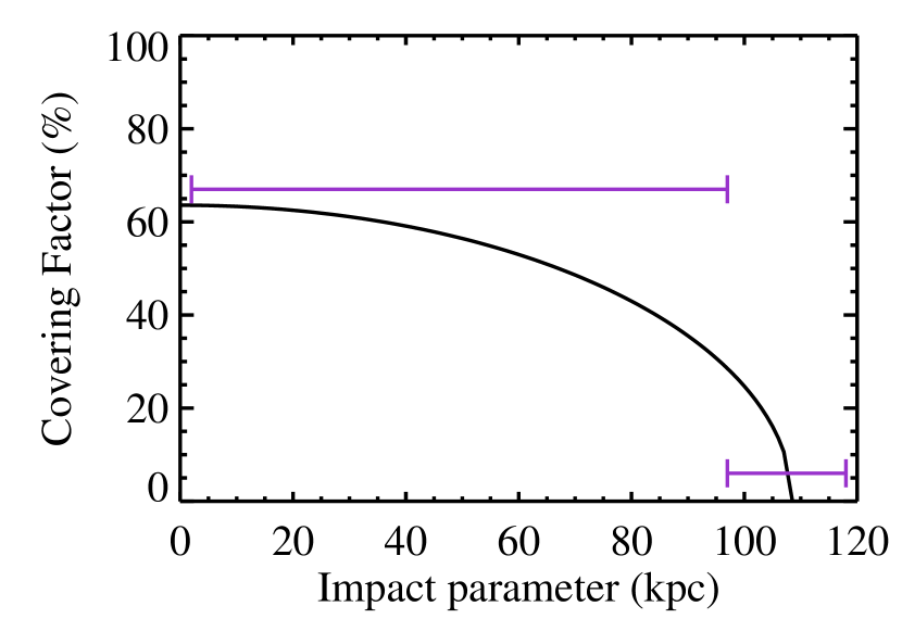
Figure 10: The covering factor to CIV absorbers as a function of impact parameter for our fiducial model galaxy at $z=0.5$ (solid line). The error bars are representative of the results of Chen et al. (2001a). The sharp truncation that is indicated by the data is roughly at $R_{\rm c}$ which is what would be expected in our model. More detailed comparisons are difficult because the data spans a wide range of redshifts and luminosities. However, with more data absorption systems will provide important constraints on the properties of the warm clouds in different mass halos.

It has long been assumed that quasar absorption systems can be identified with the gaseous content of galaxy halos (Bahcall & Spitzer, 1969). High column density systems like Lyman limit and CIV systems are observed to have nearby optical counterparts for $z<1$ (Bergeron & Boisse, 1991; Chen et al., 2001a; Chen et al., 2001b; Steidel et al., 1997; Lanzetta et al., 1995). Theoretically, these systems have been modeled as arising from warm clouds embedded within a hot galaxy halo (Mo & Miralda-Escude, 1996) in a way that is quite similar to what we describe here.

Chen et al. (2001a) find in their sample that when the impact parameter of the quasar is $<97$ kpc, $67\%$ of galaxies show CIV absorption, while when the impact parameter is $>97$ kpc, only $6\%$ of galaxies show CIV absorption systems. We compare this rough expectation to the cloud covering factor as a function of radius calculated using our fiducial parameters for a galaxy at $z=0.5$ (Figure 10). In our model there is also a sharp drop in covering factor that occurs at the cooling radius of the halo. Thus our model is in qualitative agreement with the observations.

To properly model quasar absorption systems one must be able to connect galaxy luminosity and type to a halo’s maximum circular velocity as a function of redshift. Then each observed galaxy’s gaseous halo can be modeled and compared to observations. With a great deal more absorption data it will be possible to constrain the masses and numbers of clouds in a halo as a function of halo mass and redshift. One quantity that would be useful to know is the average relationship between the column density of the absorption system and the total amount of mass along the line of sight. This should be possible combining weak gravitational lensing with a large sample of quasars and absorption systems (Maller et al., 2002), and some progress has been made on this front (Ménard & Péroux, 2003). We discuss how other properties of absorption systems may be useful in constraining the properties of the warm clouds in §10.

9 The Luminosity Function

One of the fundamental goals in galaxy formation modeling is to understand why there are so few galaxies with baryonic masses larger than $\sim 10^{11}M_{\odot}$. The cooling-time arguments (e.g. White & Rees, 1978) were originally devised with the goal of explaining this upper-mass cutoff, but it is now accepted that the cooling radius treatment alone cannot do the job in the context of modern $\Lambda$CDM cosmology (e.g. White & Frenk, 1991; Thoul & Weinberg, 1995; Somerville & Primack, 1999; Benson et al., 2003). The $\Lambda$CDM halo mass function (or velocity function) follows a near power-law distribution over the mass-scale (or velocity scale) of the Milky-Way halo (e.g. Gonzalez et al., 2000). In contrast, the luminosity function drops quickly above the luminosity scale of the Milky Way (e.g. Blanton et al., 2003). The cooling radius treatment reduces the fraction of gas that cools in high-mass halos, but only moderately, and certainly not at the level required to explain the characteristic luminosity of galaxies (see Fig. 12 below).

The issue is highlighted noticeably by the results of Bell et al. (2003) who used data from 2MASS and the SDSS to construct the baryonic mass function of stars+gas in the local universe. They concluded that the number density of galaxies falls off sharply above a cold baryonic mass of $M_{*}\simeq 10^{11}M_{\odot}$ (shaded band in Fig. 12). By integrating their mass function, they found that the total mass in cold baryons in the local universe is only $\sim 10\%$ of the total baryonic mass expected from BBN and the concordance $\Lambda$CDM model. While the original cooling arguments suggested that most of the baryonic mass would end up in stars, it seems now that most of the baryons have ended up in hot gas, or at least in some state that is not associated with central galaxies. As discussed by Benson et al. (2003), explaining the the sharp cutoff at the bright end of the luminosity function is difficult within the standard scenario without resorting to extreme conduction (above the Spitzer value) or hot super-winds with energies beyond expectation.

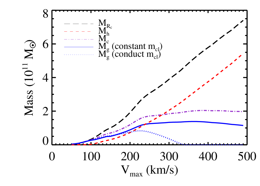
Figure 11: The total baryonic mass within the cooling radius, $M_{R_{\rm c}}$ (long-dashed line) as a function of halo $V_{\rm max}$, assuming a gas metallicity of $Z_{g}=0.1$. Also shown is total mass that we expect to have cooled, $M_{\rm c}$ (dot-dashed line) and the total mass in the hot core (short dashed line). The total cooled mass approaches a constant in high-$V_{\rm max}$ halos because much of the mass within the cooling radius ends up in a pressure-supported hot-gas core. The mass in cooled gas that accumulates into the central galaxy $M_{\rm g}$ is plotted for two different assumptions about the cloud masses. The solid line shows the resultant galaxy mass calculated assuming a constant $m_{\rm cl}=5\times 10^{10}M_{\odot}$ and the dotted line shows the result assuming that the cloud mass is set by conduction (see text).

Figure 11 shows how this problem might be alleviated by allowing a two-phase medium to develop during the cooling process. The dashed line shows the total baryonic mass within the cooling radius, $M_{R_{\rm c}}$, as a function of halo maximum circular velocity. This mass, associated with the central galaxy in the standard treatment, continues to rise rapidly as the halo velocity increases and would naively lead to a population of giant $\sim 8\times 10^{11}M_{\odot}$ galaxies associated with galaxy-group halos with $V_{\rm max}\simeq 500{\rm km}\ {\rm s}^{-1}$. The dot-dashed line, showing the total cooled mass, $M_{\rm c}=M_{R_{\rm c}}-M_{\rm h}$, determined by the two-phase treatment described in §4, is more encouraging. Interestingly, this mass approaches a characteristic value of $M_{\rm c}\simeq 2\times 10^{11}M_{\odot}$ for halos with $V_{\rm max}\lower 2.58334pt\vbox{\hbox{$\buildrel\textstyle>\over{\sim}\ $}}250{\rm km}\ {\rm s}^{-1}$.

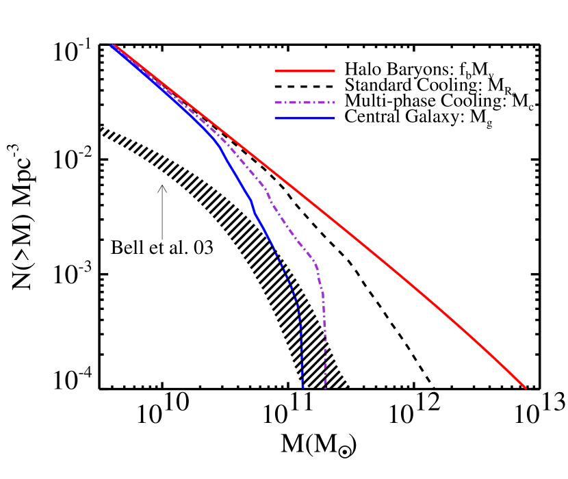
Figure 12: The cumulative baryonic mass function of galaxies reported by Bell et al. (2003) (shaded band) compared to the cumulative mass function of halo baryons (top solid line). The short-dashed line shows the (central) galaxy mass function that arises from assuming all of the mass within each halo’s cooling radius cools onto the central galaxy, $M_{R_{\rm c}}$. The dot-dashed line is the cooled mass ($M_{\rm c}$) function that arises in our picture, which allows for the presence of a hot corona in each halo (see text and Fig. 11). Finally, the lowest solid line shows the central galaxy mass function that results from modeling the survival probability of cooled clouds in the halo, assuming a typical cloud mass of $5\times 10^{6}M_{\odot}$. Only clouds that fall to the center of each halo are assumed to contribute to the central galaxy. As mentioned in the text, no merging has been accounted for in this estimate. Merging will tend to populate the massive tail of the galaxy mass function, likely bringing it even more closely in line with what is observed.

The reason why the total cooled mass approaches a constant in large halos is that the hot halo core, $M_{\rm h}$, grows rapidly with $V_{\rm max}$ because of the corresponding increase in the cooling density (short dashed line). This compensates for the increase in $M_{R_{\rm c}}$, resulting in $M_{\rm c}=M_{R_{\rm c}}-M_{\rm h}\rightarrow$ constant. Once $V_{\rm max}\lower 2.58334pt\vbox{\hbox{$\buildrel\textstyle>\over{\sim}\ $}}250{\rm km}\ {\rm s}^{-1}$, $R_{\rm c}\rightarrow$constant (Fig. 3) and $M_{\rm h}\simeq\rho_{c}R_{\rm c}^{3}\propto\rho_{c}\propto V_{\rm max}$ (see equations 18 and 12 and Fig. 2). In this regime, the total mass inside the cooling radius for our initial hot gas profile also increases proportionally to $V_{\rm max}$, so that $M_{R_{\rm c}}\propto V_{\rm max}$ as well. Therefore, both the total mass within $R_{\rm c}$ and the mass in the hot core increase with $V_{\rm max}$ in the same way (the dashed lines in Fig. 11). The amount of cooled mass remains constant at the value it had when the slopes began to match. Of course for different assumptions about the initial hot gas profile the slopes may not exactly match and the amount of cooled mass may increase (or decrease) slightly instead of remaining constant. However, it still will change much less drastically than the total mass within the cooling radius.

The solid line in Figure 11 shows our expectation for the central galaxy mass as a function of $V_{\rm max}$. This is determined using the methods outlined in §6.2, assuming a constant cloud mass of $m_{\rm cl}=5\times 10^{6}M_{\odot}$. We see that in this case, the total mass in cold gas that ends up in the central galaxy approaches a value $M_{\rm g}\simeq 1.5\times 10^{11}M_{\odot}$ for halos with $V_{\rm max}\lower 2.58334pt\vbox{\hbox{$\buildrel\textstyle>\over{\sim}\ $}}250{\rm km}\ {\rm s}^{-1}$. Of course, this treatment has not included any mergers between halos, so that this maximum galaxy mass really represents the maximum mass galaxy sitting within a relatively “quiescent” halo. An interesting implication is that forming a galaxy more massive than $\sim 1.5\times 10^{11}M_{\odot}$ would require a merger. This may be relevant in explaining why spheroidal galaxies tend to dominate the bright-end of the luminosity function.

Another possibility is that the characteristic cloud mass is not constant, but scales with the halo temperature in some way. The short-dashed line assumes that cloud masses are set by conduction ($m_{\rm cl}\propto T^{11/4}$) as described in §5.2 ( dot-dashed line in Fig. 6). In this case, cloud masses become quite large, $m_{\rm cl}\lower 2.58334pt\vbox{\hbox{$\buildrel\textstyle>\over{\sim}\ $}}10^{8}M_{\odot}$ in $V_{\rm max}\lower 2.58334pt\vbox{\hbox{$\buildrel\textstyle>\over{\sim}\ $}}300{\rm km}\ {\rm s}^{-1}$ halos. The infall time of clouds scales as $\tau_{\rm in}\propto m_{\rm cl}^{1/3}$ (equation 43, 44) and thus becomes quite long at $T$ increases. Clouds tend to remain in the hot gas halo rather than fall in to contribute to the central galaxy in this case. Interestingly, massive clouds of this type will likely be Jeans unstable in high-mass halos (e.g. Fig. 6). In this case, they may form stars and become small galaxies on their own (see our discussion in §10). As in the fixed $m_{\rm cl}$ case, giant CD galaxies could only form via mergers in this picture.

The mass function of galaxies is shown in Figure 12. The shaded band shows the baryonic mass function of galaxies in the Universe determined by Bell et al. (2003). The width of the band indicates their uncertainty (which comes mainly from the IMF). Compare this to the upper solid line, which shows the halo mass function of Sheth & Tormen (1999) scaled by the mass of baryons in each halo ($M_{\rm v}\rightarrow f_{b}M_{\rm v}$). The offset is roughly a factor of $\sim 10$ in normalization, and from this one can immediately see most of the baryons in the universe cannot be in the form of cold, galactic material. The mass function that results from assuming that all of the baryons within each halo’s cooling radius cool onto a galaxy (shown by the short-dashed line) cannot solve the problem. That is, it shows no sharp drop in galaxy counts above $\sim 10^{11}M_{\odot}$. As expected from the above discussion, the “cooled mass” function derived using our multi-phase picture does much better in accounting for this cutoff (dot-dashed line).

The mass function of gas that we expect to actually fall into the central galaxy is shown by the lowest solid line in Figure 12. In this estimate we have assumed that clouds have a typical mass of $5\times 10^{6}M_{\odot}$ (as in the solid line in Fig. 11). The high-mass cutoff compares quite well to the data in this case. We expect galaxies more massive than this cutoff to be produced solely via mergers, and we suggest that mergers will tend to populate the tail of the mass function above $\sim 10^{11}M_{\odot}$, bringing it even more in line with observations. As is clearly seen, our cooling scenario will not help explain the well-known faint-end slope problem (the low number density of galaxies smaller than $\sim 5\times 10^{10}M_{\odot}$). Of course, feedback likely plays a major role in this regime.

It is quite clear from Fig. 11 that the galaxy mass stops increasing because most of the baryons remain in the hot core. The hot gas in higher temperature, more massive halos can be observed with x-ray telescopes. These observations suggest a more complicated picture then we have been describing here; where energy injection from AGN (e.g. Omma et al., 2004) or other sources may be needed to explain the observed x-ray luminosity vrs. temperature relationship (e.g. Mushotzky & Scharf, 1997; Wu et al., 2000). Energy injection into the hot gas may also occur in galaxy mass halos. We suggest that it may not be needed to explain the high mass cutoff in the luminosity function, although undoubtedly heating processes occur to some extent.

10 Implications, Observations, and Future Work

Central to our model is the existence of a hot, low density medium that surrounds galaxies — an idea first proposed by Spitzer (1962). The hot gas density we expect for a Milky-Way type system is $n_{h}={\rho_{h}}/{\mu_{i}m_{p}}\sim 8\times 10^{-5}{\rm cm}^{-3}$ at $\sim 100$kpc. Evidence that such a corona exists has been growing in recent years. For example, gas clouds in the Magellanic Stream are more easily understood if they are confined by a hot gas medium (Stanimirović et al., 2002) as are the shapes of supergiant shells along the outer edge of the LMC (de Boer et al., 1998). Indeed, detection of H-alpha emission at the leading edges of clouds in the Magellanic Stream is best explained by ram-pressure heating from a substantial hot gas halo ($n_{h}\sim 10^{-4}{\rm{cm}}^{-3}$) at $\sim 50$kpc (Weiner & Williams, 1996). Unfortunately, most of the quantitative limits on galactic hot gas densities are model dependent, but the currently limits are at least in line with our predictions: $n_{h}\lower 2.58334pt\vbox{\hbox{$\buildrel\textstyle<\over{\sim}\ $}}(1-10)\times 10^{-5}$ cm^-3. (e.g. Snowden et al., 1997; Benson et al., 2000; Blitz & Robishaw, 2000; Moore & Davis, 1994; Murali, 2000; Tripp et al., 2003). Interestingly, Quilis & Moore (2001) argue that gas densities as low as $\sim 10^{-5}{\rm cm}^{-3}$ cannot produce the head-tail position-velocity gradients observed by Brüns et al. (2000); Brüns et al. (2001) for $\sim 20\%$ of HVCs. Our hot halo core is somewhat denser than this, so the head-tail gradients may be consistent our scenario.

One of the most promising methods for probing the hot gas halo is to observe it in absorption. Indeed, OVI in or around the Milky Way halo has been detected in this manner by FUSE (Savage et al., 2000; Sembach et al., 2003). Higher ionization lines (e.g. OVII and OVIII), can be observed by XMM-Newton and Chandra. Nicastro et al. (2002) reported the first detection of highly ionized oxygen and neon in proximity to the Local Group and similar detections have followed.

There is some debate over exactly where this absorption takes place and how the observed OVI and OVII absorbers are related (e.g. compare Sembach, 2003; Nicastro, 2003). In the context of the corona we predict, measurements to known sources in the Local Group may help avoid confusion. For example, our fiducial model predicts a column density in Hydrogen of $N_{H}=10^{19}{\rm cm^{-2}}$ along a line of sight to the LMC, assuming a distance of 50kpc. With $Z_{g}=0.1$, this gives a total expected column density in oxygen of $5.1\times 10^{14}{\rm cm^{-2}}$. At the temperature and density we expect for the Milky Way corona, most of the oxygen should be in the form of OVII (e.g. Mathur et al., 2003), but observing multiple elements and ionization lines would be useful for constraining the precise ionization state, temperature, and density of the hot medium(s) responsible for any absorption.

A related test will come from searches for metal lines associated with HVCs. Sembach et al. (2003) have argued that high-velocity OVI features observed by FUSE highlight the boundaries between warm clouds of gas and a highly extended, hot, low-density corona around the Galaxy. A related analysis suggests that these systems are associated with HVCs (Tripp et al., 2003). We would expect just this situation in our model. Note that Nicastro et al. (2003) have argued that the high-velocity OVI absorbers are better-described by a Local Group population, but they also allow for the possibility that they trace an extended Galactic corona. This second interpretation is in line with our expectations.

The soft x-ray background provides a less-direct method for probing the hot gas cores of galaxy halos. In our model, the hot-gas cores are expected to be of low density, and to have a rather low x-ray surface brightness, not directly detectable by current x-ray satellites. However, this hot gas will contribute to the soft-x-ray background. Predictions for the contribution to the soft-x-ray background may provide interesting limits on the model.

More detailed comparisons with existing and future HVC data will require more realistic models of clouds in a hot halo. The properties of clouds will need to be modeled in the presence of an ionizing background field and interactions with the hot gas background should be properly taken into account. For example, Weiner et al. (2002) have argued that measurements of H-alpha emission in HVCs can put constraints on their distances as long as H-alpha recombination is caused by photoionizing radiation from the Milky Way. Another possibility is that the H-alpha recombination is due to collisional ionization caused by ram pressure interactions with the hot gas halo. Such a scenario would be consistent with the OVI observations discussed above. Further, the ambient pressure from the hot gas halo is expected to vary as a function of radius from the halo center, and this would lead to varying cloud sizes (and densities) at fixed mass. The spectrum of HVC sizes and column densities might then be used to constrain the nature of the hot gas corona, and even to test the mass spectrum of clouds. Of course, without knowing the distances to individual HVCs, this can only be done in a statistical sense.

Searches for clouds around other galaxies will help establish whether clouds of the type we discuss are as common and numerous as we expect, and might even be used to test how cloud masses and hot core properties vary with halo mass and galaxy luminosity. Pisano et al. (2004) recently performed a search for HI clouds around three nearby galaxy groups and found that if a population of HI clouds exists around galaxies like the Milky Way, they must be clustered within 160 kpc and have HI masses $\lower 2.58334pt\vbox{\hbox{$\buildrel\textstyle<\over{\sim}\ $}}4\times 10^{5}M_{\odot}$. The clouds we expect are consistent with these limits, but should be detectable if the detection limits are relaxed only slightly. Thilker et al. (2004) have discovered a population of $\sim 50$ HI clouds around M31, with HI masses of $\sim 10^{6}M_{\odot}$. Our model would suggest that these are likely the most massive of the many thousands of clouds that should surround M31. We predict that deeper surveys with better angular resolution will find these clouds.

Quasar absorption systems provide another important avenue for determining the properties of warm clouds. While cloud populations of this type cannot be studied in detail, the study of absorption systems can probe wide range of halo types. A cross-correlation between absorbers and galaxies may yield useful information on cloud sizes, densities, and covering factors. In the future, a cross-correlation survey, similar to that of Chen et al. (2001a), but utilizing a large optical survey, would yield tight constraints on the distribution and scaling of cloud masses.

Another advantage of absorption systems is that they probe the gaseous halos of galaxies at early stages of formation, $z\sim 3$. Multi-phase cooling may be a crucial ingredient in understanding the properties of these systems. Maller et al. (2003) pointed out that a large fraction of the halo gas must be in form of warm clouds in order to explain the observed kinematics of the high-ion component in damped Lyman alpha systems (Wolfe & Prochaska, 2000). Including the multi-phase medium self-consistently will be important for precise comparisons with this data. Indeed, damped systems themselves show complex kinematics (Prochaska & Wolfe, 1997, 1998) that cannot be explained in CDM cosmologies without the presence of a large amount of gaseous substructure (Haehnelt et al., 1998; McDonald & Miralda-Escudé, 1999; Maller et al., 2001). Warm clouds may make an important contribution to this substructure, possibly after they are disrupted by tidal forces.

If pressure-supported clouds exist in the halos of most galaxies, this could be important for interpreting the flux ratios of multiply-imaged quasars (Metcalf & Madau, 2001; Dalal & Kochanek, 2002; Moustakas & Metcalf, 2003). The flux ratio anomalies have been used to argue the existence of the low-mass dark matter halos predicted by $\Lambda$CDM N-body simulations (Moore et al., 1999; Klypin et al., 1999). However, there are some indications that the fraction of mass in low-mass $\sim 10^{7}M_{\odot}$ substructures is even higher than predicted (Zentner & Bullock, 2003; Moustakas & Metcalf, 2003). The warm clouds we have described here will also cause fluctuations in the gravitational potential, and may be important. Indeed, the mass fraction in clouds is expected to be at the few percent level, and this is roughly the same as the dark matter substructure population. Fortunately, the warm clouds may also be detected by absorption in the quasar spectra so it may be possible to disentangle the two signals. Also, since the clouds are expected to be roughly constant density, they may not provide as strong a signal as the more concentrated dark matter clumps.

Multi-phase cooling might also help resolve the long-standing problem of forming disk galaxies without angular momentum loss in cosmological simulations (e.g Navarro & Steinmetz, 2000). Specifically, if cooled gas remains in warm clouds instead of settling into the galaxy, then those clouds can retain and gain angular momentum during mergers. When the clouds eventually fall in, they will produce large disks (Maller & Dekel, 2002). This scenario would be especially helpful if angular momentum in dark matter halos is predominately acquired in mergers (Maller et al., 2002; Vitvitska et al., 2002). Interestingly, Robertson et al. (2004) showed that by allowing a cold/warm medium to exist within cooled, star-forming material, they could improve the likelihood of disk formation in cosmological simulations. Specifically, the disk is more stable to its own self gravity, and less likely to fragment and loose angular momentum after it forms. Of course, this effect will only help if the material that forms the disk initially retains a large amount of angular momentum. It is in the retention of halo angular momentum that the warm/hot cloud picture becomes important. Therefore, a full multi-phase approach, with an allowance of both cold/warm and warm/hot phases, could lead to more success in this direction. However, as we mention in §11, there are significant computational challenges to overcome.

Finally, as seen in Fig. 6, the Jeans mass for a cloud decreases as a function of halo temperature, making it more likely that a cloud will collapse under its own gravity in high-temperature halos. This possibility will be more likely if the typical cloud mass increases in high-temperature halos. This is what is expected, for example, if conduction sets the characteristic cloud mass as discussed in §5.2. If a cloud’s mass exceeds the Jeans mass then it will likely fragment to form stars. It is perhaps to be expected then that there should exist a population of low-mass galaxies, born of fragmented gas in clusters, with no associated dark matter. Dwarf galaxies of this type would likely be younger than other low-mass spheroids, and have relatively low mass to light ratios by comparison.

11 Conclusions

In this paper we have taken a step towards modeling the complex realities of astrophysical hydrodynamics using a simple analytic treatment that allows the development of a two-phase warm/hot medium during gas cooling. Appealing to standard cooling instability arguments, we showed that if cooling proceeds by the formation of warm clouds embedded within a low-density hot gas background then this can explain the characteristic upper limit in the observed baryonic masses of galaxies, $\sim 10^{11}M_{\odot}$ (§9). In the standard treatment, all of the mass within the cooling radius of each halo cools onto the central galaxy, while our approach allows the survival of a hot gas core with a density close to the cooling density in each the halo. The fraction of mass that remains in the hot core component is large in high-mass halos because the cooling density is high, and this gives rise to an upper-mass limit in cooled material in these systems.

When applied to Milky-Way size halos, the standard single-phase treatment over-predicts the Milky Way mass by more than a factor of two, while our multi-phase treatment helps explain the Milky Way galaxy mass naturally, without the need for excessive feedback (§6). Because of the thermal instability, we argue that galaxy formation should proceed via the infall of warm, pressure-supported clouds. Further, if the typical cloud mass is $m_{\rm cl}\simeq 5\times 10^{6}M_{\odot}$, the residual cloud population is significant, and we identify these pressure-supported fragments with the observed High Velocity Cloud population of the Milky Way (§7). The typical Galacto-centric distance to HVCs in our picture is set by the cooling radius, $\sim 100$kpc. The same cloud mass helps explain the baryonic mass of the Milky Way, can account for high-ion absorption systems in distant galaxies (§8), and allows clouds to survive destructive processes in the halo (§5).

Including the multi-phase treatment presented here in standard semi-analytic models should be straightforward. Currently this type of modeling tracks two phases of gas: the mass contained in hot halo gas, and the mass in the “cold” central galaxy. To include the multi-phase medium, one must simply add the hot core from equation 24 to the gas in the hot phase, and include an additional accounting for warm cloud material. As sketched in equation 46, gas first cools into warm clouds and warm clouds become deposited in the central galaxy on an infall timescale. Once clouds fall in, the typical recipes for star formation may be applied, although it is likely that less feedback will be needed.

Comparison with cosmological hydrodynamic simulations may be somewhat more difficult. At present, these simulations do not resolve the multi-phase structure of halo gas, and this may lead them to predict infall rates of cooled gas that are similar to those expected from simple cooling radius arguments. In order to test these expectations, simulations would need to resolve typical cloud masses of $\sim 10^{6}M_{\odot}$ as well as properly follow cloud fragmentation in the diffuse gas halo. Yepes et al. (1997) and later Springel & Hernquist (2003) have in fact included a sub-grid model for multi-phase gas in their SPH codes, but this applies only to the star-forming, cold/warm medium. This approach seems to alleviate many of the problems faced by similar codes in the past (e.g. Robertson et al., 2004), but not the “over-cooling” problem discussed here. If the computational challenges can be overcome, hydrodynamic simulations with full multi-phase cooling may yield even more encouraging results.

In conclusion, multi-phase cooling is expected on theoretical grounds and can alleviate many of the problems that arise in the standard, single-phase procedure. The fact that warm clouds of the type predicted seem to be observed only further enforces the relevance of adopting this approach in models of galaxy formation. If we are correct, then the High-Velocity Clouds of the Milky Way are tracers of the fundamental fuel supply that governs galaxy formation in the Universe. Set in this context, the study of hot gas, HVCs, and their counterparts in external galaxies will have significant impact on how we understand galaxies and their assembly.

Appendix A A. The cooling function

$Z_{g}$	$T_{b}(10^{6}K)$	$V_{\rm max}(T_{b})$	$\alpha$	$\Lambda_{z}$
0.0	1.0	205	-0.80	0.19
0.03	2.4	307	-0.17	0.45
0.1	4.2	394	0.23	1.0
0.3	7.7	518	0.60	2.0
1.0	16.	722	1.00	4.4

Table 2: Properties of the cooling function for several different choices of hot gas metallicity, $Z_{g}$, as parameterized by the fitting function in equation A. The temperature $T_{b}$ is the temperature above which Bremsstrahlung radiation begins to dominate cooling, and $V_{\rm max}(T_{b})$ is the corresponding halo maximum circular velocity. The parameter $\alpha$ represents the fitted slope to the cooling function in the regime: $T_{r}<T<T_{m}$, where $T_{r}=1.5\times 10^{4}$K and $T_{m}\simeq 1.5\times 10^{5}$K for $Z_{g}>0$ and formally $T_{m}=T_{b}$ for $Z_{g}=0$. Finally, $\Lambda_{z}$ is the value of the cooling function in units of $2.6\times 10^{-23}{\rm cm}^{3}{\rm erg}\,{\rm s}^{-1}$ as defined in equation 13.

Astrophysical plasmas with temperatures greater than $10^{4}K$ primarily cool by radiative processes. The cooling function $\Lambda(T)$ can be calculated (e.g. Sutherland & Dopita, 1993) as a function of the gas metallicity $Z_{g}$. It is useful to introduce the dimensionless cooling function $\Lambda_{23}(T)$:

$$\Lambda(T)\equiv 10^{-23}{\rm cm}^{3}{\rm erg}\,{\rm s}^{-1}\Lambda_{23}(T)$$ (55)

Figure 1 shows $\Lambda(T,Z_{g})$ plotted as a function of temperature for five example metallicities. Note that for galaxy-sized halos ($V_{\rm max}\simeq 100-200{\rm km}\ {\rm s}^{-1}$) and mildly-enriched gas, the dimensionless cooling function takes values of order unity.

We can approximate the cooling function by a series of power-law fitting functions that captures the important scalings. For zero metallicity gas there are two important temperature regimes: $T>T_{b}$, when the dominant cooling process is Bremsstrahlung radiation, and $T_{b}>T>T_{r}=1.5\times 10^{4}$K, where the dominant cooling process is the recombination of hydrogen. For enriched gas, there is a third important temperature scale, $T_{m}$, where metal line cooling becomes important. The Bremsstrahlung region becomes important at higher temperatures for more metal rich gas, and we find that to good approximation $T_{b}=10^{6}+1.5\times 10^{7}{Z_{g}}^{2/3}$K. We also adopt $T_{m}=1.5\times 10^{5}$K.

The cooling curve is then given by,

$$\Lambda_{23}^{f}(T) = \quad 12\quad\left({{T}\over{T_{r}}}\right)^{\alpha}\hskip 28.45274ptT_{r}<T\leq T_{m}$$

$$\Lambda_{23}^{f}(T) = \Lambda_{23}^{f}(T_{m})\left({{T}\over{T_{b}}}\right)^{-1}\hskip 28.45274ptT_{m}<T\leq T_{b}$$

$$\Lambda_{23}^{f}(T) = \Lambda_{23}^{f}(T_{b})\left({{T}\over{T_{b}}}\right)^{1/3}\hskip 28.45274ptT>T_{b},$$ (56)

where $\alpha=1-\frac{1}{3}\ln{Z_{g}}$ ($Z_{g}\neq 0$), and we have added the superscript $f$ to indicate that this is a fit to the true cooling function. In the case of zero metallicity gas $\alpha=-0.8$ and the middle expression is not used (that is $T_{m}=T_{b}$). Values of $\alpha$ and $T_{b}$ for some example metallicities can be found in Table 2. This approximation is at worst good to within a factor of $3$ and is much better than that for most metallicities and temperatures.

Appendix B B. Hydrostatic Equilibrium Solutions

Here we derive the hydrostatic equilibrium solutions for gas profiles, assuming that the gravitational potential of the system is dominated by an NFW background halo. The hydrostatic force balance equation is

$$\frac{dP}{dR}=\frac{-V_{c}^{2}(R)\rho(R)}{R},$$ (57)

where $R$ is the distance from the center of the spherically-symmetric halo. The density follows that given by equation 6, and the implied rotation curve follows

$$V_{c}^{2}(R)=\frac{GM(R)}{R}=9.26c_{g}^{2}\frac{R_{s}f(R/R_{s})}{R},$$ (58)

where $f(x)\equiv\ln(1+x)-x/(1+x)$, and we adopt $c_{g}=V_{\rm max}/\sqrt{2}$ as the sound speed written in terms of the maximum circular velocity.

If we assume $P=K_{\gamma}\rho^{\gamma}$ then $K_{\gamma}=c_{g}^{2}\rho_{c}^{1-\gamma}$ and the solution to the hydrostatic equation for $\gamma\neq 1$ is

$$\rho_{g}(x)=\rho_{c}\left[1+\frac{9.26(\gamma-1)}{\gamma}\left(\frac{\ln(1+x)}{x}-\frac{\ln(1+C_{\rm c})}{C_{\rm c}}\right)\right]^{\frac{1}{\gamma-1}}.$$ (59)

For $\gamma=1$ the solution is

$$\rho_{g}(x)=\rho_{c}\exp\left[\frac{9.26}{x}\ln(1+x)-\frac{9.26}{C_{\rm c}}\ln(1+C_{\rm c})\right],$$ (60)

where $C_{\rm c}\equiv R_{\rm c}/R_{s}$. In writing this solution, we have required that the hot gas density at the cooling radius, $R_{\rm c}$, is equal to the cooling density, $\rho_{c}$. For the adiabatic assumption adopted in the paper, $\gamma=5/3$ and the solution for pressure, density, and temperature becomes

$$P_{g}(x) = P_{c}\left[1+\frac{3.7}{x}\ln(1+x)-\frac{3.7}{C_{\rm c}}\ln(1+C_{\rm c})\right]^{5/2},$$ (61)

$$\rho_{g}(x) = \rho_{c}\left[1+\frac{3.7}{x}\ln(1+x)-\frac{3.7}{C_{\rm c}}\ln(1+C_{\rm c})\right]^{3/2},$$

$$T_{g}(x) = T\left[1+\frac{3.7}{x}\ln(1+x)-\frac{3.7}{C_{\rm c}}\ln(1+C_{\rm c})\right].$$

For our adopted adiabatic profile, the pressure, temperature, and density increase slowly towards the center of the halo, reaching core values as $x\rightarrow 0$: $T_{0}=\alpha T$, $\rho_{0}=\alpha^{3/2}\rho_{c}$, and $P_{0}=\alpha^{5/2}P_{c}$ with $\alpha=4.7-3.7C_{\rm c}^{-1}\ln(1+C_{\rm c})$. For the typical range $C_{\rm c}=2-20$ we find a rather modest range of values $\alpha\simeq 2.7-4.1$. It is worth pointing out that while the central density is higher than what we have defined as the “cooling density” (set at $T=T_{c}$), it does not imply that the system is drastically unstable to cooling. Indeed, the central hot gas is likely to have reached its state of density and pressure more recently than the non-radiating gas at large radii. Moreover, for $T_{m}<T<T_{b}$, the local cooling time will scale as $\tau_{\rm cool}\propto T/\rho\Lambda(T)\propto T^{2}/\rho\propto\alpha^{1/2}$, and thus the central gas will cool more slowly than the outer halo gas.

Most of the gas, by volume, is quite close to the state at $R_{c}$. The total mass in the form of hot gas takes the form

$$M_{\rm h}=\frac{4\pi}{3}r_{c}^{3}\rho_{c}\eta_{\rm d}(C_{\rm c})$$ (62)

where the function $\eta_{\rm d}$ is determined by numerical integration to be well fitted by

$$\eta_{\rm d}(c)\simeq 1.42c^{0.3}\left[1+(c/1.65)^{1.7}\right]^{-0.24},$$ (63)

which is good to $<1\%$ for $c=1-20$, and is a rather weak function of $C_{\rm c}$: $\eta_{\rm d}\simeq 1.45-1.25$ for $C_{\rm c}=1-20$. Clearly the average gas density within $r_{c}$ will be $\bar{\rho_{h}}=\eta_{\rm d}\rho_{c}$. In the main part of the paper we work under the approximation that $\eta_{\rm d}$ is a constant and adopt a typical value of $\eta_{\rm d}=1.35$.

Similarly, we can estimate the volume-averaged pressure of the gas within $R_{\rm c}$:

$$\bar{P_{\rm h}}=\frac{4\pi\int_{0}^{R_{\rm c}}P(r)R^{2}dR}{4\pi R_{\rm c}^{3}/3}=P_{c}\eta_{P}(C_{\rm c}),$$ (64)

where the function $\eta_{P}$ is found to be well-fitted by

$$\eta_{P}\simeq 2.5c^{0.33}\left[1+(c/3.9)^{2.9}\right]^{-0.24},$$ (65)

and spans the range $\eta_{P}\simeq 2.1-3.3$ (for $C_{\rm c}=1-20$). As with the gas density, in the main part of the paper we work under the approximation that the hot gas pressure can be well-represented by a constant, with $\bar{P_{\rm h}}=\eta_{P}P_{c}$, and adopt the typical value $\eta_{P}\simeq 2.7$. The temperature profile is relatively flat, and we adopt $\bar{T_{\rm h}}=T$ throughout the paper.

References

- Arp (1985) Arp H., 1985, AJ, 90, 1012
- Bahcall & Spitzer (1969) Bahcall J. N., Spitzer L. J., 1969, ApJL, 156, L63
- Balbus (1986) Balbus S. A., 1986, ApJL, 303, L79
- Bell et al. (2003) Bell E. F., McIntosh D. H., Katz N., Weinberg M. D., 2003, ApJS, 149, 289
- Benson et al. (2003) Benson A. J., Bower R. G., Frenk C. S., Lacey C. G., Baugh C. M., Cole S., 2003, ApJ, 599, 38
- Benson et al. (2000) Benson A. J., Bower R. G., Frenk C. S., White S. D. M., 2000, MNRAS, 314, 557
- Bergeron & Boisse (1991) Bergeron J., Boisse P., 1991, A&A, 243, 344
- Binney (1977) Binney J., 1977, ApJ, 215, 483
- Birnboim & Dekel (2003) Birnboim Y., Dekel A., 2003, MNRAS, 345, 349
- Blanton et al. (2003) Blanton M. R., et al., 2003, ApJ, 592, 819
- Blitz (2002) Blitz L., 2002, in ASP Conf. Ser. 254: Extragalactic Gas at Low Redshift, p. 215
- Blitz & Robishaw (2000) Blitz L., Robishaw T., 2000, ApJ, 541, 675
- Blitz et al. (1999) Blitz L., Spergel D. N., Teuben P. J., Hartmann D., Burton W. B., 1999, ApJ, 514, 818
- Blumenthal et al. (1984) Blumenthal G. R., Faber S. M., Primack J. R., Rees M. J., 1984, Nature, 311, 517
- Brüns et al. (2000) Brüns C., Kerp J., Kalberla P. M. W., Mebold U., 2000, A&A, 357, 120
- Brüns et al. (2001) Brüns C., Kerp J., Pagels A., 2001, A&A, 370, L26
- Bregman (1980) Bregman J. N., 1980, ApJ, 236, 577
- Bryan & Norman (1998) Bryan G. L., Norman M. L., 1998, ApJ, 495, 80
- Bullock et al. (2001) Bullock J. S., Dekel A., Kolatt T. S., Kravtsov A. V., Klypin A. A., Porciani C., Primack J. R., 2001, ApJ, 555, 240
- Bullock et al. (2001) Bullock J. S., Kolatt T. S., Sigad Y., Somerville R. S., Kravtsov A. V., Klypin A. A., Primack J. R., Dekel A., 2001, MNRAS, 321, 559
- Burkert & Lin (2000) Burkert A., Lin D. N. C., 2000, ApJ, 537, 270
- Chandran & Cowley (1998) Chandran B. D. G., Cowley S. C., 1998, Physical Review Letters, 80, 3077
- Chandrasekhar (1961) Chandrasekhar S., 1961, Hydrodynamic and hydromagnetic stability. International Series of Monographs on Physics, Oxford: Clarendon
- Chen et al. (2001a) Chen H., Lanzetta K. M., Webb J. K., 2001a, ApJ, 556, 158
- Chen et al. (2001b) Chen H., Lanzetta K. M., Webb J. K., Barcons X., 2001b, ApJ, 559, 654
- Cole et al. (2000) Cole S., Lacey C. G., Baugh C. M., Frenk C. S., 2000, MNRAS, 319, 168
- Cowie & McKee (1977) Cowie L. L., McKee C. F., 1977, ApJ, 211, 135
- Dalal & Kochanek (2002) Dalal N., Kochanek C. S., 2002, ApJ, 572, 25
- de Boer et al. (1998) de Boer K. S., Braun J. M., Vallenari A., Mebold U., 1998, A&A, 329, L49
- de Heij et al. (2002) de Heij V., Braun R., Burton W. B., 2002, A&A, 392, 417
- Dehnen & Binney (1998) Dehnen W., Binney J., 1998, MNRAS, 294, 429
- Doroshkevich & Zeldovich (1981) Doroshkevich A. G., Zeldovich I. B., 1981, Zhurnal Eksperimental noi i Teoreticheskoi Fiziki, 80, 801
- Fall & Rees (1985) Fall S. M., Rees M. J., 1985, ApJ, 298, 18
- Field (1965) Field G. B., 1965, ApJ, 142, 531
- Frenk et al. (1999) Frenk C. S., et al., 1999, ApJ, 525, 554
- Gnat & Sternberg (2004) Gnat O., Sternberg A., 2004, ApJ, 608, 229
- Gonzalez et al. (2000) Gonzalez A. H., Williams K. A., Bullock J. S., Kolatt T. S., Primack J. R., 2000, ApJ, 528, 145
- Gunn & Gott (1972) Gunn J. E., Gott J. R. I., 1972, ApJ, 176, 1
- Haehnelt et al. (1998) Haehnelt M. G., Steinmetz M., Rauch M., 1998, ApJ, 495, 647
- Hatton et al. (2003) Hatton S., Devriendt J. E. G., Ninin S., Bouchet F. R., Guiderdoni B., Vibert D., 2003, MNRAS, 343, 75
- Helly et al. (2003) Helly J. C., Cole S., Frenk C. S., Baugh C. M., Benson A., Lacey C., Pearce F. R., 2003, MNRAS, 338, 913
- Helmi et al. (2003) Helmi A., White S. D. M., Springel V., 2003, MNRAS, 339, 834
- Hernquist & Springel (2003) Hernquist L., Springel V., 2003, MNRAS, 341, 1253
- Katz (1992) Katz N., 1992, ApJ, 391, 502
- Keres et al. (2004) Keres D., Katz N., Davé R., Weinberg D. H., astro-ph/0407095
- Kim & Narayan (2003) Kim W., Narayan R., 2003, ApJL, 596, L139
- Klypin et al. (2001) Klypin A., Kravtsov A. V., Bullock J. S., Primack J. R., 2001, ApJ, 554, 903
- Klypin et al. (1999) Klypin A., Kravtsov A. V., Valenzuela O., Prada F., 1999, ApJ, 522, 82
- Klypin et al. (2002) Klypin A., Zhao H., Somerville R. S., 2002, ApJ, 573, 597
- Lacey & Cole (1993) Lacey C., Cole S., 1993, MNRAS, 262, 627
- Landau & Lifshitz (1959) Landau L. D., Lifshitz E. M., 1959, Fluid Mechanics. Pergamaon, New York
- Lanzetta et al. (1995) Lanzetta K. M., Bowen D. V., Tytler D., Webb J. K., 1995, ApJ, 442, 538
- Lin & Murray (1992) Lin D. N. C., Murray S. D., 1992, ApJ, 394, 523
- Lin & Murray (2000) Lin D. N. C., Murray S. D., 2000, ApJ, 540, 170
- Ménard & Péroux (2003) Ménard B., Péroux C., 2003, A&A, 410, 33
- Malagoli et al. (1996) Malagoli A., Bodo G., Rosner R., 1996, ApJ, 456, 708
- Maller & Dekel (2002) Maller A. H., Dekel A., 2002, MNRAS, 335, 487
- Maller et al. (2002) Maller A. H., Dekel A., Somerville R., 2002, MNRAS, 329, 423
- Maller et al. (2002) Maller A. H., Kolatt T. S., Bartelmann M., Blumenthal G. R., 2002, ApJ, 569, 72
- Maller et al. (2001) Maller A. H., Prochaska J. X., Somerville R. S., Primack J. R., 2001, MNRAS, 326, 1475
- Maller et al. (2003) Maller A. H., Prochaska J. X., Somerville R. S., Primack J. R., 2003, MNRAS, 343, 268
- Maloney & Putman (2003) Maloney P. R., Putman M. E., 2003, ApJ, 589, 270
- Mathur et al. (2003) Mathur S., Weinberg D. H., Chen X., 2003, ApJ, 582, 82
- McDonald & Miralda-Escudé (1999) McDonald P., Miralda-Escudé J., 1999, ApJ, 519, 486
- McKee & Begelman (1990) McKee C. F., Begelman M. C., 1990, ApJ, 358, 392
- Metcalf & Madau (2001) Metcalf R. B., Madau P., 2001, ApJ, 563, 9
- Miura (1984) Miura A., 1984, J. Gerophys. Res., 89, 801
- Mo & Miralda-Escude (1996) Mo H. J., Miralda-Escude J., 1996, ApJ, 469, 589
- Moore & Davis (1994) Moore B., Davis M., 1994, MNRAS, 270, 209
- Moore et al. (1999) Moore B., Ghigna S., Governato F., Lake G., Quinn T., Stadel J., Tozzi P., 1999, ApJL, 524, L19
- Moustakas & Metcalf (2003) Moustakas L. A., Metcalf R. B., 2003, MNRAS, 339, 607
- Muller et al. (1963) Muller C. A., Oort J. H., Raimond E., 1963, CR Acad. Sci. Paris, 257, 1661
- Murali (2000) Murali C., 2000, ApJL, 529, L81
- Murray & Lin (1990) Murray S. D., Lin D. N. C., 1990, ApJ, 363, 50
- Murray & Lin (1992) Murray S. D., Lin D. N. C., 1992, ApJ, 400, 265
- Murray & Lin (2004) Murray S. D., Lin D. N. C., 2004, astro-ph/0407411
- Murray et al. (1993) Murray S. D., White S. D. M., Blondin J. M., Lin D. N. C., 1993, ApJ, 407, 588
- Mushotzky & Scharf (1997) Mushotzky R. F., Scharf C. A., 1997, ApJL, 482, L13
- Nagashima & Yoshii (2004) Nagashima M., Yoshii Y., 2004, astro-ph/0404485
- Narayan & Medvedev (2001) Narayan R., Medvedev M. V., 2001, ApJL, 562, L129
- Navarro et al. (1995) Navarro J. F., Frenk C. S., White S. D. M., 1995, MNRAS, 275, 56
- Navarro & Steinmetz (2000) Navarro J. F., Steinmetz M., 2000, ApJ, 538, 477
- Nicastro (2003) Nicastro F., 2003, astro-ph/0311162
- Nicastro et al. (2002) Nicastro F., Zezas A., Drake J., Elvis M., Fiore F., Fruscione A., Marengo M., Mathur S., Bianchi S., 2002, ApJ, 573, 157
- Nicastro et al. (2003) Nicastro F., Zezas A., Elvis M., Mathur S., Fiore F., Cecchi-Pestellini C., Burke D., Drake J., Casella P., 2003, Nature, 421, 719
- Omma et al. (2004) Omma H., Binney J., Bryan G., Slyz A., 2004, MNRAS, 348, 1105
- Oort (1966) Oort J. H., 1966, Bull. Astron. Inst. Netherlands, 18, 421
- Pisano et al. (2004) Pisano D. J., Barnes D., Gibson B., Staveley-Smith L., Freeman K., Kilborn V., 2004, astro-ph/0406278
- Primack (2002) Primack J. R., 2002, in Cline D., ed., Proceedings of 5th International UCLA Symposium on Sources and Detection of Dark Matter, Nucl. Phys. B
- Prochaska & Wolfe (1997) Prochaska J. X., Wolfe A. M., 1997, ApJ, 487, 73
- Prochaska & Wolfe (1998) Prochaska J. X., Wolfe A. M., 1998, ApJ, 507, 113
- Putman et al. (2002) Putman M. E., et al., 2002, AJ, 123, 873
- Quilis & Moore (2001) Quilis V., Moore B., 2001, ApJL, 555, L95
- Rees & Ostriker (1977) Rees M. J., Ostriker J. P., 1977, MNRAS, 179, 541
- Robertson et al. (2004) Robertson B., Yoshida N., Springel V., Hernquist L., 2004, ApJ, 606, 32
- Savage et al. (2000) Savage B. D., et al., 2000, ApJL, 538, L27
- Sembach (2003) Sembach K. R., 2003, astro-ph/0311089
- Sembach et al. (2004) Sembach K. R., et al., 2004, ApJS, 150, 387
- Sembach et al. (2003) Sembach K. R., Wakker B. P., Savage B. D., Richter P., Meade M., Shull J. M., Jenkins E. B., Sonneborn G., Moos H. W., 2003, ApJS, 146, 165
- Shapiro & Field (1976) Shapiro P. R., Field G. B., 1976, ApJ, 205, 762
- Sheth & Tormen (1999) Sheth R. K., Tormen G., 1999, MNRAS, 308, 119
- Silk (1977) Silk J., 1977, ApJ, 211, 638
- Snowden et al. (1997) Snowden S. L., et al., 1997, ApJ, 485, 125
- Somerville & Primack (1999) Somerville R. S., Primack J. R., 1999, MNRAS, 310, 1087
- Somerville et al. (2001) Somerville R. S., Primack J. R., Faber S. M., 2001, MNRAS, 320, 504
- Spergel et al. (2003) Spergel D. N., et al., 2003, ApJS, 148, 175
- Spitzer (1962) Spitzer L., 1962, Physics of Fully Ionized Gases. Physics of Fully Ionized Gases, New York: Interscience
- Spitzer (1978) Spitzer L., 1978, Physical processes in the interstellar medium. New York: Wiley-Interscience
- Springel & Hernquist (2003) Springel V., Hernquist L., 2003, MNRAS, 339, 289
- Springel et al. (2001) Springel V., White S. D. M., Tormen G., Kauffmann G., 2001, MNRAS, 328, 726
- Stanimirović et al. (2002) Stanimirović S., Dickey J. M., Krčo M., Brooks A. M., 2002, ApJ, 576, 773
- Steidel et al. (1997) Steidel C. C., Dickinson M., Meyer D. M., Adelberger K. L., Sembach K. R., 1997, ApJ, 480, 568
- Sternberg et al. (2002) Sternberg A., McKee C. F., Wolfire M. G., 2002, ApJS, 143, 419
- Sutherland & Dopita (1993) Sutherland R. S., Dopita M. A., 1993, ApJS, 88, 253
- Tasitsiomi et al. (2003) Tasitsiomi A., Kravtsov A. V., Gottloeber S., Klypin A. A., 2003, astro-ph/0311062
- Thilker et al. (2004) Thilker D. A., Braun R., Walterbos R. A. M., Corbelli E., Lockman F. J., Murphy E., Maddalena R., 2004, ApJL, 601, L39
- Thoul & Weinberg (1995) Thoul A. A., Weinberg D. H., 1995, ApJ, 442, 480
- Tripp et al. (2003) Tripp T. M., et al., 2003, AJ, 125, 3122
- van den Bosch et al. (2003) van den Bosch F. C., Abel T., Hernquist L., 2003, MNRAS, 346, 177
- van Woerden et al. (1999a) van Woerden H., Schwarz U. J., Peletier R. F., Wakker B. P., Kalberla P. M. W., 1999a, Nature, 400, 138
- van Woerden et al. (1999b) van Woerden H., Schwarz U. J., Peletier R. F., Wakker B. P., Kalberla P. M. W., 1999b, in IAU Symp. 186: Galaxy Interactions at Low and High Redshift, p. 58
- Verschuur (1969) Verschuur G. L., 1969, ApJ, 156, 771
- Vietri et al. (1997) Vietri M., Ferrara A., Miniati F., 1997, ApJ, 483, 262
- Vitvitska et al. (2002) Vitvitska M., Klypin A. A., Kravtsov A. V., Wechsler R. H., Primack J. R., Bullock J. S., 2002, ApJ, 581, 799
- Wakker et al. (2001) Wakker B. P., Kalberla P. M. W., van Woerden H., de Boer K. S., Putman M. E., 2001, ApJS, 136, 537
- Wakker & van Woerden (1991) Wakker B. P., van Woerden H., 1991, A&A, 250, 509
- Wechsler et al. (2002) Wechsler R. H., Bullock J. S., Primack J. R., Kravtsov A. V., Dekel A., 2002, ApJ, 568, 52
- Weiner et al. (2002) Weiner B. J., Vogel S. N., Williams T. B., 2002, in ASP Conf. Ser. 254: Extragalactic Gas at Low Redshift ,p. 256
- Weiner & Williams (1996) Weiner B. J., Williams T. B., 1996, AJ, 111, 1156
- White & Frenk (1991) White S. D. M., Frenk C. S., 1991, ApJ, 379, 52
- White & Rees (1978) White S. D. M., Rees M. J., 1978, MNRAS, 183, 341
- Wolfe & Prochaska (2000) Wolfe A. M., Prochaska J. X., 2000, ApJ, 545, 591
- Wu et al. (2000) Wu K. K. S., Fabian A. C., Nulsen P. E. J., 2000, MNRAS, 318, 889
- Yepes et al. (1997) Yepes G., Kates R., Khokhlov A., Klypin A., 1997, MNRAS, 284, 235
- Yoshida et al. (2002) Yoshida N., Stoehr F., Springel V., White S. D. M., 2002, MNRAS, 335, 762
- Zakamska & Narayan (2003) Zakamska N. L., Narayan R., 2003, ApJ, 582, 162
- Zentner & Bullock (2003) Zentner A. R., Bullock J. S., 2003, ApJ, 598, 49