[Feedback]Feedback Processes at Cosmic DawnFerrara, A. & Salvaterra, R.
SISSA/ISAS, Via Beirut 4, 34014 Trieste, Italy

The word “feedback” is by far one of the most used ones in modern cosmology where it is applied to a vast range of situations and astrophysical objects. However, for the same reason, its meaning in the context is often unclear or fuzzy. Hence a review on feedback should start from setting the definition of feedback on a solid basis. We have found quite useful to this aim to go back to the Oxford Dictionary from where we take the following definition:

Fee’dback n. 1. (Electr.) Return of fraction of output signal from one stage of circuit, amplifier, etc. to input of same or preceding stage (positive, negative, tending to increase, decrease the amplification, etc). 2. (Biol., Psych., etc) Modification or control of a process or system by its results or effects, esp. by difference between the desired and actual results.

In spite of the broad description, we find this definition quite appropriate in many ways. First, the definition outlines the fact that the concept of feedback invokes a back reaction of a process on itself or on the causes that have produced it. Secondly, the character of feedback can be either negative or positive. Finally, and most importantly, the idea of feedback is intimately linked to the possibility that a system can become self-regulated. Although some types of feedback processes are disruptive, the most important ones in astrophysics are probably those that are able to drive the systems towards a steady state of some sort. To exemplify, think of a galaxy which is witnessing a burst of star formation. The occurrence of the first supernovae will evacuate/heat the gas thus suppressing the star formation activity. Such feedback is then acting back on the energy source (star formation); it is of a negative type, and it could regulate the star formation activity in such a way that only a sustainable amount of stars is formed (regulation). However, feedback can fail to produce such regulation either in small galaxies where the gas can be ejected by the first SNe or in cases when the star formation timescale is too short compared to the feedback one. As we will see there are at least three types of feedback, and even the stellar feedback described in the example above is part of a larger class of feedback phenomena related to the energy deposition of massive stars. We then start by briefly describing the key physical ingredients of feedback processes in cosmology.

1 Shock Waves

A shock represents a “hydrodynamic surprise”, in the sense that such a wave travels faster than signals in the fluid, which are bound to propagate at the gas sound speed, $c_{s}$. It is common to define the shock speed, $v_{s}$, in terms of $c_{s}$ by introducing the shock Mach number, $M$:

$$v_{s}=Mc_{s}=M(\gamma P/\rho)^{1/2},$$ (1)

where $P$ and $\rho$ are the gas pressure and density, respectively. The change of the fluid velocity $v$ is governed by the momentum equation

$$\rho\frac{\partial v}{\partial t}+\rho v\cdot\nabla v=-\nabla P-\frac{1}{8\pi}\nabla B^{2}+\frac{1}{4\pi}B\cdot\nabla B,$$ (2)

where $B$ is the magnetic field. The density is determined by the continuity equation

$$\frac{\partial\rho}{\partial t}+v\cdot\nabla\rho=-\rho\nabla v.$$ (3)

1.1 Hydrodynamics of Shock Waves

The large-scale properties of a shock in a perfect gas, with $B=0$ are fully described by the three ratios $v_{2}/v_{1}$ $\rho_{2}/\rho_{1}$ and $P_{2}/P_{1}$, determined in terms of the conditions ahead of the shock (i.e. $v_{1}$, $\rho_{1}$ and $P_{1}$) by the Rankine-Hugoniot jump conditions resulting from matter, momentum and energy conservation:

$$\rho_{1}v_{1}=\rho_{2}v_{2},$$ (4)

$$P_{1}+\rho_{1}v_{1}^{2}=P_{2}+\rho_{2}v_{2}^{2},$$ (5)

$$v_{2}(\frac{1}{2}\rho_{2}v_{2}^{2}+U_{2})-v_{1}(\frac{1}{2}\rho_{1}v_{1}^{2}+U_{1})=v_{1}P_{1}-v_{2}P_{2},$$ (6)

where $U$ is the internal energy density of the fluid. If the fluid behaves as a perfect gas on each side of the front we have $U=P/(\gamma-1)$.

In the adiabatic limit it is sufficient to consider the mass and momentum equations only. By solving such system we obtain:

$$\frac{v_{2}}{v_{1}}=\frac{\rho_{1}}{\rho_{2}}=\frac{\gamma-1}{\gamma+1}+\frac{2}{\gamma+1}\frac{1}{M^{2}},$$ (7)

where the Mach number is defined as $M^{2}=v_{1}^{2}/c_{1}^{2}$ and $c_{1}$ is the sound velocity in the unperturbed medium ahead of the shock. For strong shocks, i.e. $M\gg 1$ and $\gamma=5/3$, $\rho_{2}/\rho_{1}=4$ and

$$T_{2}=\frac{3\mu}{16k}v_{s}^{2},$$ (8)

where $v_{s}=v_{1}-v_{2}$

In the isothermal limit, i.e. when the cooling time of the postshock gas becomes extremely short and the initial temperature is promptly re-established,

$$\frac{\rho_{2}}{\rho_{1}}=\frac{v_{1}^{2}}{c_{s}^{2}}=M^{2},$$ (9)

where $c_{s}$ is the sound velocity on both sides of the shock. While in the adiabatic case the compression factor is limited to four, in an isothermal shock much larger compressions are possible due to the softer equation of state characterizing the fluid.

1.2 Hydromagnetic Shock Waves

Assuming $B$ is parallel to the shock front (so that $B\cdot\nabla B=0$), eq. (5) can be replaced by

$$P_{1}+\rho_{1}v_{1}^{2}+\left(\frac{B_{1}^{2}}{8\pi}\right)=P_{2}+\rho_{2}v_{2}^{2}+\left(\frac{B_{2}^{2}}{8\pi}\right).$$ (10)

Magnetic flux conservation requires $B_{1}/\rho_{1}=B_{2}/\rho_{2}$, so that in the adiabatic limit the magnetic pressure $B^{2}/8\pi$ increases by only a factor 16.

In the isothermal limit the compression depends only linearly on the Alfvénic Mach number $M_{a}$

$$\frac{\rho_{2}}{\rho_{1}}=\sqrt{2}\frac{v_{1}}{v_{a,1}}=M_{a},$$ (11)

where $v_{a}=B/\sqrt{4\pi\rho_{1}}$ is the Alfvén velocity. Hence, some of the shock kinetic energy is stored in the magnetic field lines rather than being used to compress the gas as in the field-free case; in other words a magnetized gas is less compressible than an unmagnetized one.

1.2.1 Structure of Radiative Shocks

The structure of a shock can be divided into four regions (McKee & Draine 1991). The radiative precursor is the region upstream of the shock in which radiation emitted by the shock acts as a precursor of the shock arrival. The shock front is the region in which the relative kinetic energy difference of the shocked and unshocked gas is dissipated. If the dissipation is due to collisions among the atoms or molecules of the gas, the shock is collisional. On the other hand, if the density is sufficiently low that collisions are unimportant and the dissipation is due to the collective interactions of the particles with the turbulent electromagnetic fields, the shock is collisionless. Next comes the radiative zone, in which collisional processes cause the gas to radiate. The gas cools and the density increases. Finally, if the shock lasts long enough, a thermalization region is produced, in which radiation from the radiative zone is absorbed and re-radiated.

1.3 Supernova Explosions

In the explosion of a supernova three different stages in the expansion may be distinguished. In the initial phase the interstellar material has little effect because of its low moment of inertia; the velocity of expansion of the supernova envelope will then remain nearly constant with time. This phase terminates when the mass of the swept up gas is about equal to the initial mass $M_{e}$ expelled by the supernova, i.e. $(4\pi/3)r_{s}^{3}\rho_{1}=M_{e}$, where $\rho_{1}$ is the density of the gas in front of the shock and $r_{s}$ is the radius of the shock front. For $M_{e}=0.25\;M_{\odot}$ and $\rho_{1}=2\times 10^{-24}$ g/cm³, $r_{s}\simeq 1$ pc, which will occurs about 60 yr after the explosion. During the second phase (Sedov-Taylor phase) the mass behind the shock is determined primarily by the amount of interstellar gas swept up, but the energy of this gas will remain constant. When radiative cooling becomes important (radiative phase), the temperature of the gas will fall to a relatively low value. The motion of the shock is supported by the momentum of the outward moving gas and the shock may be regarded as isothermal. The velocity of the shell can be computed from the condition of momentum conservation (snowplow model). This phase continues until $v_{s}=\max\{v_{t},c_{s}\}$, where $v_{t}$ is the turbulent velocity of the gas, when the shell loses its identity due to gas random motions.

1.3.1 Blastwave Evolution

To describe the evolution of a blastwave, the so-called thin shell approximation is frequently used. In this approximation, one assumes that most of the mass of the material swept up during the expansion is collected in a thin shell. We start by applying (we neglect the ambient medium density and shell self-gravity) the virial theorem to the shell:

$$\frac{1}{2}\frac{d^{2}I}{dt^{2}}=2E=2(E_{k}+E_{t}),$$ (12)

where $I$ is the moment of inertia, and $E_{k}$ ($E_{t}$) is the kinetic (thermal) energy of the shell. Let us introduce the structure parameter $K$ in the following form:

$$K=\frac{1}{MRv_{2}}\int_{0}^{R}dm\,rv,$$ (13)

where $M$ is the ejected mass, $R$ the shell radius. Substituting in equation (12) with $v=v_{2}(r/R)$, we obtain

$$K\frac{d}{dt}(Mrv_{s})=2E(v_{s}/v_{2}).$$ (14)

To recover the Sedov-Taylor adiabatic phase we integrate up to $R$ and assume $\rho(R)=\rho_{0}R^{-m}$, $E=const.$, $K=(6-2m)/(7-2m)$

$$R(t)=\left[\frac{(5-m)E}{\pi\rho_{0}K}\right]^{1/(5-m)}t^{2/(5-m)}.$$ (15)

The previous expression can be obtained also via a dimensional approach. In fact, in the adiabatic phase the energy is conserved and hence

$$E\propto Mv_{s}^{2}\propto\rho_{0}R^{5-m}t^{-2},$$ (16)

so that

$$R^{5-m}\propto\frac{E}{\rho_{0}}t^{2};$$ (17)

the fraction of the total energy transformed in kinetic form is

$$E_{k}=\frac{1}{2}KM\left(\frac{3}{4}v_{s}^{2}\right)=\frac{3E}{2(5-m)}.$$ (18)

We note that in the limit of a homogeneous ambient medium ($m=0$) we recover the standard Sedov-Taylor evolution $R\propto t^{2/5}$, with 30% of the explosion energy in kinetic form.

A similar reasoning can be followed to recover the radiative phase behavior. In this phase $v_{2}=v_{s}$, i.e. the shock wave is almost isothermal and $K=1$, i.e. the shell is thin. Under these assumptions the energy is lost at a rate

$$\dot{E}=-4\pi R^{2}\left(\frac{1}{2}\rho_{0}v_{s}^{2}\right).$$ (19)

There are two possible solutions of equation (12) in this case: (a) the pressure-driven snowplow in which

$$R(t)\propto t^{2/(7-m)},$$ (20)

or the momentum-conserving solution

$$R(t)\propto t^{1/(4-m)}.$$ (21)

In both cases, the expansion proceeds at a lower rate with respect to the adiabatic phase.

In order to study the evolution of an explosion in a more realistic way it is necessary to resort to numerical simulations as the one shown in Figure 1. From there the inner structure of the remnant is clearly visible: indeed most of the mass is concentrated in a thin shell (located at about 80 pc after 0.5 Myr from the explosion); a reverse shock is also seen which is proceeding towards the center and thermalizing the ejecta up to temperatures of the order of $10^{7}$ K. In between the two shocks is the contact discontinuity between the ejecta and the ambient medium, through which the pressure remains approximately constant.

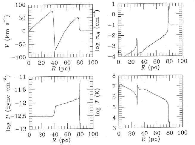
Figure 1: The structure of spherical supernova remnant calculated using a high-resolution numerical hydrodynamical code. The remnant age is $t=5\times 10^{5}$ yr. This Figure is taken from Cioffi, McKee & Bertschiger (1988)

2 Photoionization

The ionization balance equation around a source is given by

$$4\pi R^{2}n\frac{dR}{dt}+\frac{4}{3}\pi R^{3}n^{2}\alpha=4\pi S_{i}(0),$$ (22)

where $S_{i}(0)$ is the ionizing photon rate from the source, $n$ is the neutral gas density and $\alpha$ is the recombination coefficient. The solution of the ionization balance equation is

$$R(t)=R_{S}[1-\exp(-2n\alpha t/3)]^{1/3}.$$ (23)

As time goes to infinity the radius tends to the Stromgren radius

$$R_{S}=\left(\frac{3S_{i}(0)}{\alpha n^{2}}\right)^{1/3}.$$ (24)

The above equations implies that $R_{S}$ is reached in

$$t_{S}=\frac{3}{2}n\alpha\simeq 2\times 10^{5}n\mbox{ yr},$$ (25)

and the typical ionization front (I-front) velocity is $v_{I}\propto S_{i}(0)/R^{2}n$.

Depending on the value of $v_{I}$ we can distinguish three types of I-fronts, where $c_{i}$ ($c_{n}$) is the sound speed in the ionized (neutral) gas:

1. R(arefied)-TYPE: $v_{I}>(c_{i},c_{n})$

2. Strong D(ense)-TYPE: $c_{n}<v_{I}<c_{i}$

3. Weak D(ense)-TYPE: $v_{I}<(c_{i},c_{n})$

In the case of R-TYPE I-front there is no hydrodynamical reaction to the passage of the ionizing front, since the its motion is supersonic relative to the gas behind as well as ahead of the front. In the case of D-TYPE fronts the dynamical timescale becomes short enough for the gas to react to photoionization and a shock will form and precede the ionizing front thus increasing the ambient gas density.

2.0.1 Photoionization Equilibrium

It is convenient to divide the ionizing flux into two parts, a ‘stellar’ part $S(\nu)$, resulting directly from the input radiation from the star, and a ‘diffuse’ part $S_{d}(\nu)$, resulting from the emission of the ionized gas, that in a pure H gas is due to recombinations into 1² S state.

$$S_{t}(\nu)=S(\nu)+S_{d}(\nu).$$ (26)

Both the recombination radiation and photoionization cross section ($\sigma\propto\nu^{3}$) are peaked at the threshold, $\nu_{L}$. We can identify two approximate cases (Osterbrok 1989):

1. MENZEL CASE A: optically thin nebula, i.e. $\tau(\nu=\nu_{L})=n_{H}\sigma(\nu_{L})R<1$, and the diffuse photons can escape;

2. MENZEL CASE B: optically thick nebula, i.e. diffuse photons are absorbed very close to the point at which they are generated (‘on-the-spot’ approximation).

Menzel case B is usually a good approximation for many astrophysical purposes because the diffuse radiation-field photons have $\nu\simeq\nu_{L}$, and therefore a short mean free path before absorption. Under the hypothesis of the on-the-spot approximation, the recombination coefficient is given by

$$\alpha_{eff}=\alpha-\alpha_{1S},$$ (27)

resulting roughly in a 60% decrease. The physical meaning is that in optically thick nebulae, the ionizations caused by stellar radiation-field photons are balanced by recombinations to excited levels of H, while recombinations to the ground level generate ionizing photons that are absorbed elsewhere in the nebula but have no net effect on the overall ionization balance.

3 Thermal Instability

A final crucial ingredient to understand feedback and self-regulation is represented by the thermal instability. Let us rewrite the usual mass, momentum and energy equations in a slightly different form (Balbus 1995):

$$\frac{d\ln\rho}{dt}+\rho\nabla\cdot v=0,$$ (28)

$$\rho\frac{dv}{dt}=-\nabla P,$$ (29)

$$\frac{3}{2}P\frac{d\ln P}{dt}\rho^{-5/3}=-\rho L(\rho,T),$$ (30)

where $L$ is the net cooling function (i.e. heating-cooling) and is taken to be a function of density and temperature; in the equilibrium state $v=L=0$. We perturb the equilibrium by introducing small disturbance. We write such perturbations as $\delta q\propto\mbox{e}^{(kr+nt)}$; $nt$ is then the growth rate of the instability. The linearized system yields the dispersion relation

$$n^{3}+\frac{2}{3}T\Theta_{T,\rho}n^{2}+k^{2}c_{s}^{2}n+\frac{2}{5}k^{2}c_{s}^{2}T\Theta_{T,\rho}=0,$$ (31)

where $\Theta\equiv(\rho/P)L$ and $\Theta_{A,B}\equiv(\partial\Theta/\partial A)_{B}$.

For large $k$ (small wavelengths) the instability occurs isobarically, that is pressure is kept approximately constant as the density increases following the process of condensation and cooling. In this case such equations has three solutions:

$$n_{1}=-\frac{2}{5}T\Theta_{T,P},$$ (32)

$$n_{2,3}=\pm ikc_{s}-\frac{2}{15}T\Theta_{T,S}.$$ (33)

It is straightforward to recognize that $n_{2,3}$ are the modified sound wave modes, whereas $n_{1}$ corresponds to the condensation mode. Note also that the sign of the temperature derivative of the cooling function determines whether or not a mode is unstable (instability occurs if $\Theta_{T,P}<0$).

In the opposite (isochoric) limit characterized by small $k$ (large wavelengths), the condensation mode has the following expression:

$$n_{1}=-\frac{2}{3}T\Theta_{T,\rho},$$ (34)

Although formally a solution of the dispersion equation, the thermal instability cannot physically occur under isochoric conditions. The reason is that on such large scales there is not enough time to establish pressure equilibrium as the cooling time is much shorter than the sound crossing time over a wavelength. Thus the density remains approximately constant while the gas cools, and pressure equilibrium is likely to be restored promptly and rather dramatically by a propagating shock front.

To better understand the nature of the thermal instability let us plot the curve of the equilibrium solution $L=0$ in the $P-T$ plane for a hypothetical cooling function (Figure 2). Above the curve, heating dominates over cooling; below $L=0$, the gas is cooled. Between $P_{min}$ and $P_{max}$ a constant pressure line will intersect the curve in three points (A, B, and C); A and B are thermally stable. This is readily understood since a small isobaric increase (decrease) in temperature at either of these points takes the system into the cooling (heating) region of the $P-T$ plane from where it is immediately driven back to equilibrium position. On the other hand, a small increase (decrease) in the temperature in the unstable point B takes one into the heating (cooling) region, with the result that the system is driven yet further from its equilibrium. This leads to the coexistence of two (or more) thermodynamic phases and provides the main argument to interpret the multiphase medium commonly observed in galaxies and in cosmic gas. We will see later on how this concept is closely linked with the self-regulation connected to feedback processes.

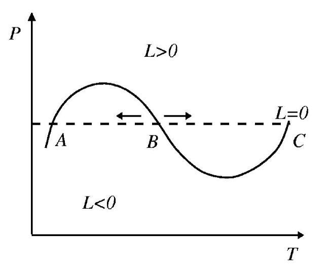
Figure 2: Equilibrium solution curve $L=0$ in the $P-T$ plane for a hypothetical cooling function. See text.

4 The Need for Feedback in Cosmology

One of the main aims of physical cosmology is to understand in detail galaxy formation starting from the initial density fluctuation field with a given spectrum (typically a CDM one). Such ab initio computations require a tremendous amount of physical processes to be included before it becomes possible to compare their predictions with experimental data. In particular, it is crucial to model the interstellar medium of galaxies, which is know to be turbulent, have a multi-phase thermal structure, can undergo gravitational instability and form stars. To account for all this complexity, in addition one should treat correctly all relevant cooling processes, radiative and shock heating (let alone magnetic fields!). This has proven to be essentially impossible even with present day best supercomputers. Hence one has to resort to heuristic models where simplistic prescriptions for some of these processes must be adopted. Of course such an approach suffers from the fact that a large number of free parameters remains which cannot be fixed from first principles. These are essentially contained in each of the ingredients used to model galaxy formation, that is, the evolution of dark halos, cooling and star formation, chemical enrichment, stellar populations. Fortunately, there is a large variety of data against which the models can be tested: these data range from the fraction of cooled baryons to cosmic star formation histories, the luminous content of halos, luminosity functions and faint galaxy counts. The feedback processes enter the game as part of such iterative try-and-learn process to which we are bound by our ignorance in dealing with complex systems as the galaxies. Still, we are far from a full understanding of galaxies in the framework of structure formation models. The hope is that feedback can help us to solve some “chronic” problems found in cosmological simulations adopting the CDM paradigm. Their (partial) list includes:

1. Overcooling: the predicted cosmic fraction of cooled baryons is larger than observed. Moreover models predict too many faint, low mass galaxies;

2. Disk Angular Momentum: the angular momentum loss is too high and galactic disk scale lengths are too small;

3. Halo Density Profiles: profiles are centrally too concentrated;

4. Dark Satellites: too many satellites predicted around our Galaxy.

4.1 The Overcooling Problem

Among the various CDM problems, historically the overcooling has been the most prominent and yet unsolved one. In its original formulation it has been first spelled out by White & Frenk (1991). Let us assume that, as a halo forms, the gas initially relaxes to an isothermal distribution which exactly parallels that of the dark matter. The virial theorem then relates the gas temperature $T_{vir}$ to the circular velocity of the halo $V_{c}$,

$$kT_{vir}=\frac{1}{2}\mu m_{p}V_{c}^{2}\mbox{ or }T_{vir}=36V^{2}_{c,km/s}\mbox{K},$$ (35)

where $\mu m_{p}$ is the mean molecular weight of the gas. At each radius in this distribution we can then define a cooling time as the ratio of the specific energy content to the cooling rate,

$$t_{cool}(r)=\frac{3\rho_{g}(r)/2\mu m_{p}}{n_{e}^{2}(r)\Lambda(T)},$$ (36)

where $\rho_{g}(r)$ is the gas density profile and $n_{e}(r)$ is the electron density. $\Lambda(T)$ is the cooling function. The cooling radius is defined as the point where the cooling time is equal to the age of the universe, i.e. $t_{cool}(r_{cool})=t_{Hubble}=H(z)^{-1}$.

Considering the virialized part of the halo to be the region encompassing a mean overdensity is 200, its radius and mass are defined by

$$r_{vir}=0.1H_{0}^{-1}(1+z)^{3/2}V_{c},$$ (37)

$$M_{vir}=0.1(GH_{0})^{-1}(1+z)^{3/2}V_{c}^{3}.$$ (38)

Let us distinguish two limiting cases. When $r_{cool}\gg r_{vir}$ (accretion limited case), cooling is so rapid that the infalling gas never comes to hydrostatic equilibrium. The supply of cold gas for star formation is then limited by the infall rate rather than by cooling. The accretion rate is obtained by differentiating equation (38) with respect to time and multiplying by the fraction of the mass of the universe that remains in gaseous form:

$$\dot{M}_{acc}=f_{g}\Omega_{g}\frac{d}{dt}0.1(GH_{0})^{-1}(1+z)^{3/2}V_{c}^{3}=0.15f_{g}\Omega_{g}G^{-1}V_{c}^{3}.$$ (39)

Note that, except for a weak time dependence of the fraction of the initial baryon density which remains in gaseous form, $f_{g}$, this infall rate does not depend on redshift.

In the opposite limit, $r_{cool}\ll r_{vir}$ (quasi-static case), the accretion shock radiates only weakly, a quasi-static atmosphere forms, and the supply of cold gas for star formation is regulated by radiative losses near $r_{cool}$. A simple expression for the inflow rate is

$$\dot{M}_{qst}=4\pi\rho_{g}(r_{cool})r_{cool}^{2}\frac{d}{dt}r_{cool}.$$ (40)

The gas supply rates predicted by equations (39) and (40) are illustrated in Figure 3. In any particular halo, the rate at which cold gas becomes available for star formation is the minimum between $\dot{M}_{acc}$ and $\dot{M}_{qst}$.

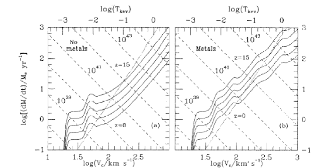
Figure 3: Gas infall rate and cooling rates in dark matter halos as a function of circular velocity and redshift. The infall rate (dotted line) is essentially independent of redshift; the cooling rates (solid lines) are given for redshift $z=0,1,3,7$ and 15 (from bottom to top). Dashed lines give present-day X-ray luminosities in erg s^-1 produced by gas cooling at the given rate in each halo. The predicted temperature of this emission is given on the upper abscissa. (a) A cooling function for gas of zero metallicity is assumed. (b) A cooling function for metal enriched gas. This Figure is taken from White & Frenk (1991).

According to the models of Thomas et al. (1986), the bolometric X-ray luminosity of the region within the cooling radius of a galactic cooling flow is

$$L_{X}=2.5\dot{M}_{cool}V_{c}^{2}.$$

The predictions of this formula are superposed on Figure 3 (dashed lines). For large circular velocities the mass cooling rates correspond to quite substantial X-ray luminosities.

Integrating the gas supply rates $\dot{M}_{cool}$ over redshift and halo mass distribution, we find that for $\Omega_{b}=0.04$ most of the gas is used before the present time. This is unacceptable, since the density contributed by the observed stars in galaxies is less than 1% of the critical density. So, the star formation results to be too rapid without a regulating process, i.e. feedback.

To solve this puzzle, Larson (1974) proposed that the energy input from young stars and supernovae could quench star formation in small protogalaxies before more than a small gas fraction has been converted into stars.

Stellar energy input would counteract radiative losses in the cooling gas and tend to reduce the supply of gas for further star formation. We can imagine that the star formation process is self-regulating in the sense that the star formation rate $\dot{M}_{\star}$ takes the value required for heating to balance dissipation in the material which does not form stars. This produces the following prescription for the star formation rate:

$$\dot{M}_{\star}(V_{c},z) = \epsilon(V_{c})\mbox{min}(\dot{M}_{acc},\dot{M}_{qst}),$$ (41)

$$\epsilon(V_{c}) = [1+\epsilon_{0}(V_{0}/V_{c})^{2}]^{-1}.$$ (42)

For large $V_{c}$ the available gas turns into stars with high efficiency because the energy input is not sufficient to prevent cooling and fragmentation; for smaller objects the star formation efficiency $\epsilon$ is proportional to $V_{c}^{2}$. The assumption of self regulation at small $V_{c}$ seems plausible because the time interval between star formation and energy injection is much shorter than either the sound crossing time or the cooling time in the gaseous halos. However, other possibilities can be envisaged. For example, Dekel & Silk (1986) suggested that supernovae not only would suppress cooling in the halo gas but would actually expel it altogether. The conditions leading to such an event are discussed next.

4.2 Dwarf Galaxies: a Feedback Lab

The observation of dwarf galaxies has shown well-defined correlations between their measured properties, and in particular

1. Luminosity-Radius $L\propto R^{r}$ with $r=4$

2. Luminosity-Metallicity $L\propto Z^{z}$ with $z=5/2$

3. Luminosity-Velocity dispersion $L\propto V^{v}$ with $v=4$

A simple model can relate the observed scaling parameters $r$, $z$, and $v$ to each other (Dekel & Silk 1986). Consider a uniform cloud of initial mass $M_{i}=M_{g}+M_{\star}$ ($M_{g}$ is the mass of gas driven out of the system, and $M_{\star}$ is the mass in stars) in a sphere of radius $R_{i}$ which undergoes star formation. The metallicity for a constant yield in the instantaneous recycling approximation is given by $Z=y\ln(1+M_{\star}/M_{g})$ where $y$ are the yields.

Let us impose simple scaling relations: $M_{i}\propto M$ (gas mass proportional to the dark matter mass), $R\simeq R_{i}$ , and $V\simeq V_{i}$ (gas loss has no dynamical effect). From the observed scaling relation we have $L\propto R^{r}\propto V^{v}$. Now we should write the analogous relations for structure and velocity that hold before the removal, i.e. $M_{i}\propto R^{ri}$ and $M_{i}\propto V^{vi}$.

Consider now the case in which the gas is embedded in a dark halo, and assume that when it forms stars the mass in gas is proportional to the dark matter inside $R_{i}$, $M_{i}\propto M$. If the halo is dominant, the gas loss would have no dynamical effect on the stellar system that is left behind, so $R\simeq R_{i}$ and $V\simeq V_{i}$. The relations for structure and velocity that hold before the removal give

$$L\propto R^{r}\propto V^{v},\;\;M\propto R^{ri},\;\;V^{2}\propto M/R,$$ (43)

so that we obtain

$$v=2r/(ri-1).$$ (44)

In the limit $M_{\star}\ll M_{g}$ and $L\propto M_{\star}$, from the metallicity relation we have

$$Z\propto\frac{M_{\star}}{M_{g}}\propto\frac{L}{M}\propto L^{1/z},$$ (45)

so that

$$r/ri=(z-1)/z.$$ (46)

The final equation comes from the energy condition. For thermal energy, in the limit of substantial gas loss, $M_{g}\simeq M_{i}$, we have $L\propto MV^{2}$, and so

$$v=2z.$$ (47)

For a CDM spectrum $P(k)=Ck^{n_{s}}$, we obtain $r_{i}=6/(5+n_{s})$ and introducing $z=2r/(r-1)$ and $n_{s}=12/(r+1)-5$. For $r=4$ we find $n_{s}=-2.6$ consistent with the CDM and the scaling relations are

$$L\propto R^{4}\propto Z^{2.7}\propto V^{5.3}.$$ (48)

Let us now investigate the critical conditions, in terms of gas density $n$ and virial velocity $V$, for a global supernova-driven gas removal from a galaxy while it is forming stars. Here, spherical symmetry and the presence of a central point source are assumed. The basic requirement for gas removal is that the energy that has been pumped into the gas is enough to expel it from the protogalaxy. The energy input in turn depends on the supernova rate, on the efficiency of energy transfer into the gas, and on the time it takes for the SNRs to overlap and hence affect a substantial fraction of the gas. The first is determined by the rate of star formation, the second by the evolution of the individual SNRs, and the third by both. When all these are expressed as a function of $n$ and $V$, the critical condition for removal takes the form

$$E(n,V)\geq\frac{1}{2}M_{g}V^{2}.$$ (49)

This relation defines a locus in the $n-V$ diagram shown in Figure 5 within which substantial gas loss is possible. In Figure 5, the cooling curve, above which the cooling time is less than the free-fall time, confines the region where the gas can contract and form stars. The almost vertical line $V_{crit}$ divides the permissible region for galaxy formation in two; a protogalaxy with $V>V_{crit}$ would not expel a large fraction of its original gas but rather turn most of its original gas into stars to form a ‘normal’ galaxy. A protogalaxy with $V<V_{crit}$ can produce a supernova-driven wind out of the first burst of star formation, which would drive a substantial fraction of the protogalactic gas out, leaving a diffuse dwarf.

The short-dashed curve marked “1$\sigma$” corresponds to density perturbations $\delta M/M$ at their equilibrium configuration after a dissipationless collapse from a CDM spectrum, normalized to $\delta M/M$ at a comoving radius $8h^{-1}$ Mpc. The density $n$ is calculated for a uniformly distributed gas in the CDM halos, with a gas-to-total mass ratio $\chi=0.1$. The corresponding parallel short-dashed curve corresponds to the protogalactic gas clouds, after a contraction by a factor $\chi^{-1}=10$ inside isothermal halos, to densities such that star formation is possible. The vertical dashed arrow marks the largest galaxy that can form out of a typical 1$\sigma$ peak in the initial distribution of density fluctuations. The vast majority of such protogalaxies, when they form stars, have $V<V_{crit}$, so they would turn into dwarfs. The locus where “normal” galaxies are expected to be found is the shaded area. It is evident that most of them must originate form 2$\sigma$ and 3$\sigma$ peaks in the CDM perturbations.

So, the theory hence predicts two distinct types of galaxies which occupy two distinct loci in the $n-V$ diagram: the “normal” galaxies are confined to the region of larger virial velocities and higher densities, and they tend to be massive; while the diffuse dwarfs are typically of smaller velocities and lower densities, and their mass in star is less than $5\times 10^{9}\;M_{\odot}$.

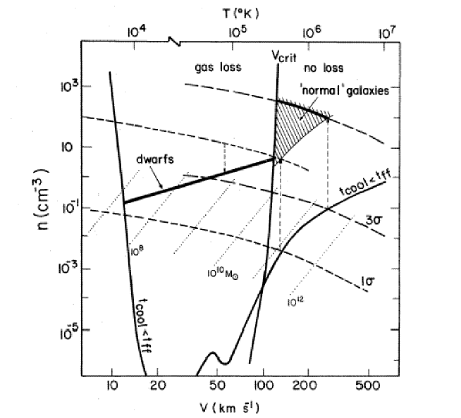
Figure 4: Gas number density vs. virial velocity (or viral temperature), the formation of dwarf vs. ‘normal’ galaxies in CDM halos, and the origin of biased galaxy formation. This Figure is taken from Dekel & Silk (1986).

This simple model, in spite of its enlightening power, has clear limitations. The most severe is that is assumes a spherical geometry and a single supernova explosion. These assumptions have been released by a subsequent study based on a large set of numerical simulations (Mac-Low & Ferrara 1999). These authors modelled the effects of repeated supernova explosions from starbursts in dwarf galaxies on the interstellar medium of these galaxies, taking into account the gravitational potential of their dominant dark matter halos. They explored supernova rates from one every 30,000 yr to one every 3 Myr, equivalent to steady mechanical luminosities of $L=0.1-10\times 10^{38}$ ergs s^-1, occurring in dwarf galaxies with gas masses $M_{g}=10^{6}-10^{9}M_{\odot}$. Surprisingly, Mac-Low & Ferrara (1999) found that the mass ejection efficiency is very low for galaxies with mass $M_{g}\geq 10^{7}M_{\odot}$. Only galaxies with $M_{g}\mathrel{\hbox to0.0pt{\lower 3.0pt\hbox{$\sim$}\hss}\raise 2.0pt\hbox{$<$}}10^{6}M_{\odot}$ have their interstellar gas blown away, and then virtually independently of $L$ (see Table 1). On the other hand, metals from the supernova ejecta are accelerated to velocities larger than the escape speed from the galaxy far more easily than the gas. They found that for $L_{38}=1$, only about 30% of the metals are retained by a $10^{9}M_{\odot}$ galaxy, and virtually none by smaller galaxies (see Table 2).

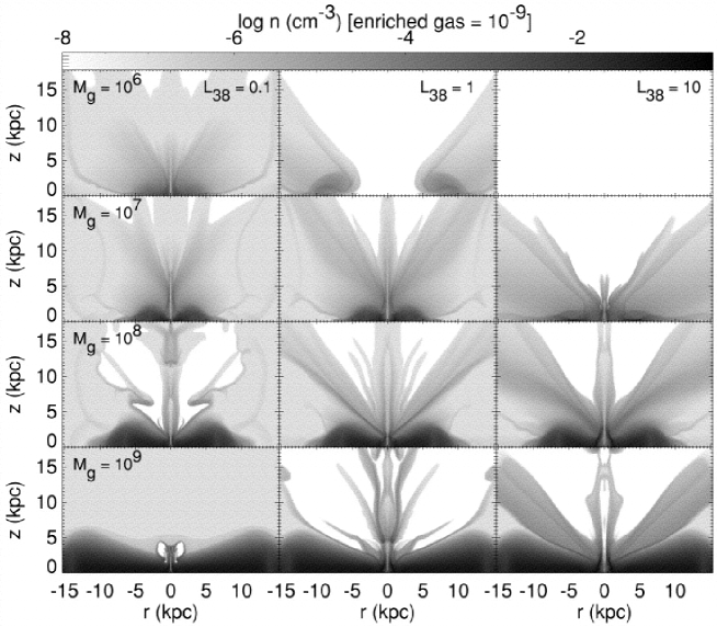
Figure 5: Distribution of metal-enriched stellar outflow material and SN ejecta from the starburst energy source at time 200 Myr. Note that in most cases, no enriched gas remains in the disks of the galaxies. This Figure is taken from Mac-Low & Ferrara (1999).

Visible Mass	Mechanical Luminosity [$10^{38}$ erg s-1]
[$M_{\odot}$]	0.1	1.0	10
$10^{6}$	0.18	1.0	1.0
$10^{7}$	$3.5\times 10^{-3}$	$8.4\times 10^{-3}$	$4.8\times 10^{-2}$
$10^{8}$	$1.1\times 10^{-4}$	$3.4\times 10^{-4}$	$1.3\times 10^{-3}$
$10^{9}$	$0.0$	$7.6\times 10^{-6}$	$1.9\times 10^{-5}$

Table 1: Mass ejection efficiency

Visible Mass	Mechanical Luminosity [$10^{38}$ erg s-1]
[$M_{\odot}$]	0.1	1.0	10
$10^{6}$	1.0	$1.0$	1.0
$10^{7}$	1.0	$1.0$	1.0
$10^{8}$	0.8	$1.0$	1.0
$10^{9}$	0.0	$0.69$	0.97

Table 2: Metal ejection efficiency

4.3 Blowout, Blowaway and Galactic Fountains

The results of the MacLow & Ferrara study served to clearly classify the various events induced by starburst in galaxies. We can distinguish between blowout and blowaway processes, depending on the fraction of the parent galaxy mass involved in the mass loss phenomena. Whereas in the blowout process the fraction of mass involved is the one contained in cavities created by the supernova or superbubble explosions, the blowaway is much more destructive, resulting in the complete expulsion of the gas content of the galaxy. The two processes lie in different regions of the $(1+\phi)-M_{g,7}$ plane shown in figure 6, where $\phi=M_{h}/M_{g}$ is the dark-to-visible mass ratio and $M_{g,7}=M_{g}/10^{7}\;M_{\odot}$ (Ferrara & Tolstoy 2000). Galaxies with gas mass content larger than $10^{9}\;M_{\odot}$ do not suffer mass losses, due to their large gravitational well. Of course, this does not rule out the possible presence of outflows with velocities below the escape velocity (fountain) in which material is temporarily stored in the halo and then returns to the main body of the galaxy. For galaxies with gas mass lower than this value, outflows cannot be prevented. If the mass is reduced further, and for $\phi\mathrel{\hbox to0.0pt{\lower 3.0pt\hbox{$\sim$}\hss}\raise 2.0pt\hbox{$<$}}20$, a blowavay, and therefore a complete stripping of the galactic gas, should occur. To exemplify, the expected value of $\phi$ as function of $M_{g}$ empirically derived by Persic et al. (1996) is also plotted, which should give an idea of a likely location of the various galaxies in the $(1+\phi)-M_{g,7}$ plane.

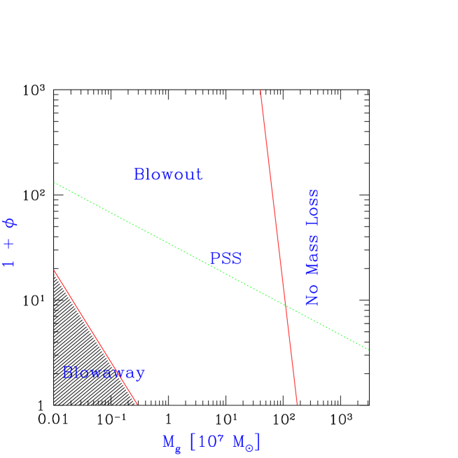
Figure 6: Regions in the $(1+\phi)-M_{g,7}$ plane in which different dynamical phenomena may occur. Also shown is the locus point describing the Persic et al. (PSS) relation (dotted line). This Figure is taken from Ferrara & Tolstoy (2000).

4.3.1 Blowout

The evolution of a point explosion in an exponentially stratified medium can be obtained from dimensional analysis. Suppose that the gas density distribution is horizontally homogeneous and that $\rho(z)=\rho_{0}\exp(-z/H)$. The velocity of the shock wave is $v\sim(P/\rho)^{1/2}$, where the pressure $P$ is roughly equal to $E/z^{3}$, and $E$ is the total energy if the explosion. Then it follows that

$$v(z)\simeq E^{1/2}\rho_{0}^{-1/2}\exp(z/2H)z^{-3/2}.$$ (50)

This curve has a minimum at $z=3H$ and this value defines the height at which the shock wave, initially decelerating, is accelerated to infinity and a blowout takes place. Therefore, $3H$ can be used as the fiducial height where the velocity $v_{b}=v(3H)$ is evaluated.

There are three different possible fates for SN-shocked gas, depending on the value of $v_{b}$. If $v_{b}<c_{s,eff}$, where $c_{s}$ is the sound speed in the ISM, then the explosion will be confined in the disk and no mass-loss will occur; for $c_{s,eff}<v_{b}<v_{e}$ ($v_{e}$ is the escape velocity) the supershell will breakout of the disk into the halo, but the flow will remain bound to the galaxy; finally, $v_{e}<v_{b}$ will lead to a true mass-loss from the galaxy.

4.3.2 Blowaway

The requirement for blowaway is that the momentum of the shell is larger than the momentum necessary to accelerate the gas outside the shell at velocity larger than the escape velocity, $M_{s}v_{c}\leq M_{0}v_{e}$. Defining the disk axis ratio as $\epsilon=R/H\geq 1$, the blowaway condition can be rewritten as

$$\frac{v_{b}}{v_{e}}\geq(\epsilon-a)^{2}a^{-2}\mbox{e}^{3/2},$$ (51)

where $a=2/3$. The above equation is graphically displayed in Figure 7. Flatter galaxies (large $\epsilon$ values) preferentially undergo blowout, whereas rounder ones are more likely to be blown-away; as $v_{b}/v_{e}$ is increased the critical value of $\epsilon$ increases accordingly. Unless the galaxy is perfectly spherical, blowaway is always preceded by blowout; between the two events the aspect of the galaxy may look extremely perturbed, with one or more huge cavities left after blowout.

Figure 7: Conditions for blowaway, blowout and confinement as a function of the major-to-minor axis ratio $\epsilon$ of dwarf galaxies; $\epsilon=1$ corresponds to spherical bodies. This Figure is taken from Ferrara & Tolstoy (2000).

4.4 Further Model Improvements

All models discussed so far make the so-called SEX BOMB assumption, i.e. a Spherically EXpanding blastwave. This is a good assumption as long as a single burst regions exists whose size is small compared to the size of the system and it is located at the center of the galaxy. This however is a rather idealized situation.

A more detailed study about the possibility of mass loss due to distributed SN explosions at high redshift has been carried on by Mori, Ferrara & Madau (2002). These authors presented results from three–dimensional numerical simulations of the dynamics of SN–driven bubbles as they propagate through and escape the grasp of subgalactic halos with masses $M=10^{8}\,h^{-1}\,M_{\odot}$ at redshift $z=9$. Halos in this mass range are characterized by very short dynamical timescales (and even shorter gas cooling times) and may therefore form stars in a rapid but intense burst before SN ‘feedback’ quenches further star formation. This hydrodynamic simulations use a nested grid method to follow the evolution of explosive multi–SN events operating on the characteristic timescale of a few $\times 10^{7}\,$yr, the lifetime of massive stars. The results confirm that, if the star formation efficiency of subgalactic halos is $\approx 10\%$, a significant fraction of the halo gas will be lifted out of the potential well (‘blow–away’), shock the intergalactic medium, and pollute it with metal–enriched material, a scenario recently advocated by Madau, Ferrara, & Rees (2001). Depending on the stellar distribution, Mori et al. (2002) found that less than 30% of the available SN energy gets converted into kinetic energy of the blown away material, the remainder being radiated away.

However, it appears that realistic models lead to the conclusion that mechanical feedback is less efficient than expected from SEX BOMB simple schemes. The reason is that off–nuclear SN explosions drive inward–propagating shocks that tend to collect and pile up cold gas in the central regions of the host halo. Low–mass galaxies at early epochs then may survive multiple SN events and continue forming stars.

Figure 8 and 9 show the fraction of the initial halo baryonic mass contained inside (1, 0.5, 0.1) of the virial radius $r_{vir}$ as a function of time for two different runs: an extended stellar distribution (case 1) and a more concentrated one (case 2). The differences are striking: in case 1, the amount of gas at the center is constantly increasing, finally collecting inside 0.1$r_{vir}$ about 30% of the total initial mass. On the contrary, in case 2, the central regions remain practically devoided of gas until 60 Myr, when the accretion process starts. The final result is a small core containing a fraction of only 5% of the initial mass. In the former case, 50% of the halo mass is ejected together with the shell, whereas in case 2 this fraction is $\sim 85$%, i.e., the blow-away is nearly complete.

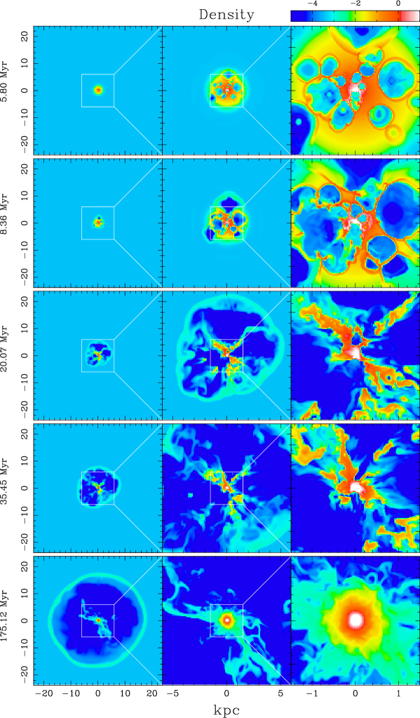
Figure 8: Snapshots of the logarithmic number density of the gas at five different elapsed times. The three panels in each row show the spatial density distribution in the $x-y$ plane on the nested grids. The density range is $-5\leq\log(n/\mbox{cm}^{-3})\leq 1$. This Figure is taken from Mori et al. (2002)

Figure 9: The evolution of the gas mass inside the gravitational potential well of the CDM halo for an extended stellar distribution (case 1) as a function of time. Curves correspond to the gas mass inside the virial radius $r_{\rm vir}$ (solid line), $0.5r_{\rm vir}$ (dashed line), and $0.1r_{\rm vir}$ (dotted line). This Figure is taken from Mori et al. (2002).

Figure 10: The same of Figure 9 but for a more concentrated stellar distribution (case 2). This Figure is taken from Mori et al. (2002).

As a first conclusion, it seems that quenching star formation in galaxies by ejecting large fraction of their gas seems very difficult and hence unviable as a feedback scheme (although this might be possible in very small galaxies). Heavy elements can instead escape much more easily as they are carried away by the mass-unloaded, hot, SN-shocked gas; energy is carried away efficiently as well. This conclusion raises the issue if star formation must be rather governed by more gentle and self-regulating processes, i.e. a ‘true’ feedback.

5 The Gentle Feedback

In numerical simulations an astonishingly large number of attempts to implement feedback scheme have been tried. In spite of this wealth, essentially all of them can be classified in one of the two following categories: (i) ‘Thermal’ feedback schemes in which the energy released by a supernova is assumed to simply heat the ISM. The dynamics of the gas is only slightly affected: this is because the dense gas in star-forming region is able to radiate away this heat input very quickly. Moreover it would imply a huge amount of hot gas, that is hardly seen in local universe. (ii) ‘Kinetic’ feedback schemes, in which the explosion energy is assigned to fluid parcels as pure kinetic energy. This algorithm performs slightly better and it is probably more physical. It would be impossible to review in detail here even only a few of these schemes. We have thus chosen to describe a minimum feedback model that tries to catch the most important feature that is missing in the previous ones, that is the multiphase structure and the matter exchange among gas phases characterizing real galaxies.

5.1 Feedback as ISM Sterilization

Dynamical models of the interstellar medium (ISM) describe this complex system in terms of a dense, cold neutral component (CNM) co-spatial with a warm neutral intercloud medium (WNM) by which it is pressure confined. Such a multiphase medium offers an efficient self-regulatory mechanism for star formation. Schematically, as more stars are formed, the extra heating caused by the enhancement of their UV field tends to transfer mass from the CNM into the WNM, where the conditions are highly unfavorable to star formation, i.e. a sterile phase. This acts to decrease the star formation rate and slowly brings back gas from the WNM reservoir in the cold phase where stars can start to form again. Under most conditions this cycle is stable and tends to regulate the amount of gas turned in stars quite effectively. In this scenario starburst can be only produced either by external triggers (mergings and interactions with other galaxies) and/or during the very first phase of galaxy formation, when the gentle feedback has not yet had the time to control the system. The physical basis of the gentle feedback is the thermal instability already discussed early on. Field (1965) discussed the criteria for stability of gas in thermal equilibrium (i.e. $L(n,T)=n\Gamma(n,T)-n^{2}\Lambda(n,T)=0$, see also sect. 3). In a plot of the thermal pressure $P/k$ versus the hydrogen density $n$, the region of thermal stability occur for $d(\log P)/d(\log n)>0$. Thus, Figure 11 shows that a stable two-phase medium, can be maintained in pressure equilibrium for $P_{min}<P<P_{max}$. For pressure less than $P_{min}$ only the warm phase is possible, while at pressures greater than $P_{max}$ only the cold phase is possible (Wolfire et al. 1995). Moreover, in Figure 11 it is shown, that when the metallicity of the gas $Z$, assumed to be equal to the dust-to-gas ratio $D/G$, is decreased, the pressure range in which a multiphase medium can exist becomes wider; in addition, the mean equilibrium pressure and density of the cold gas increase (Ricotti et al. 1997).

The first advantage of such feedback scenario is that there is no need for gas loss as required by canonical feedback schemes: typically, the loss rate necessary to regulate the star formation activity is difficult to sustain for galaxies with mass of the order of the Milky Way for interestingly long periods. In addition, the production of large amounts of hot, X-ray emitting gas is expected. Such gas is rarely seen in/around observed galaxies.

An additional advantage of these models is the self-regulatory behavior of the process, that we have seen to be typical of feedback. In fact, there is no need of infall or outflow of gas from the galaxy (close box). As cold gas is available, the galaxy has a star formation burst, leading to the increase of the metallicity and of the dust content. Moreover, extra heating is provided by the SN explosions and from UV background, so that some gas mass is transferred from the CNM to the WIM. The star formation is quenched since the gas is in the warm, sterile phase, and the heating drops down. After a cooling time, the gas becomes again available for star formation.

The disadvantage of these models is that they are physically complex, since the involve the interplay between dynamics and thermodynamics. Hence, a number of physical processes await inclusion in current cosmological simulations.

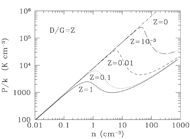
Figure 11: Thermal pressure $P/k$ vs. hydrogen density $n$; the curves refer to different values of the dust-to-gas ratio, $D/G$, and metallicity $Z$, with $D/G=Z$. The gas is thermally stable for $(d\log P/d\log n)>0$ (i.e. positive slope of the curves). Unless $Z=0$, a stable two-phase medium is supported. This Figure is taken from Ricotti et al. (1997).

5.2 A Porosity-regulated Feedback

A similar feedback scheme has been recently proposed by Silk (2003). In such a feedback prescription, the filling factor of the hot, SN-shocked gas plays a central role. The filling factor $f_{hot}$ of hot gas can be expressed in terms of the porosity $Q$ as

$$f_{hot}=1-\mbox{e}^{-Q},$$ (52)

where $Q$ is regulated by the pressure confinement of the supernova bubbles. As $f_{hot}\rightarrow 1$, the star formation rate reaches a saturation level and for $f=1$ a ‘buoyant’ wind is produced with outflow rate approximately equal to the star formation rate.

This feedback has the advantage to be based on the physical treatment of the supernova explosion, that current numerical simulations fail to follow in detail due to the lack of resolution. Moreover the expression of the porosity $Q$ is identical for all the masses: the outflow rate is of the order of the star formation rate. Only the star formation efficiency depends on potential well depth ($\epsilon_{cr}\propto V_{c}^{2.7}$). The wind efficiency depends only weakly on $V_{c}$. In summary, outflows can occur even for massive galaxies since star formation efficiency is larger in these systems.

However, there are some problems. The porosity-driven feedback is not a true multiphase model and has to be generalized to include the time evolution of $Q$, metallicity, UV background, etc. Moreover, it again implies a large amount of hot gas that is not detected in galaxies.

5.3 Advanced Multiphase/Feedback Schemes

The main problem affecting numerical simulations of feedback processes is that, owing to the limited numerical resolution, there is a large disparity between the minimum simulation timescale and the true physical timescale associated with supernova feedback (Thacker & Couchman 2001). Physically, following a supernova event, the gas cooling time very rapidly increases to $O(10^{7})$ yr over the time it takes the shock front to propagate. Thus, it is the timescale - $t_{\dot{E}}$ - for the cooling time to increase markedly that is of critical importance. In the SPH simulations, ‘stars’ form and ‘supernova feedback’ occurs in gas cores that are typically less than $h_{min}/5$ in diameter ($h_{min}$ being the effective spatial resolution). Any rearrangement of the particles in such a small region leads to a density estimate varying by at most $\sim 7$%. Since the cooling time in the model is dependent on the local SPH density, any energy deposited into a feedback region only reduces the local cooling rate by increasing the temperature; the SPH density cannot respond on a timescale that in real supernova events would very rapidly increase the cooling time. A successful feedback algorithm in an SPH model must thus overcome the fact that $\rho_{SPH}$ does not change on the same timescale as $t_{\dot{E}}$ and consequently that cooling times for dense gas cores remain short.

Standard implementations of SPH overestimate the density for particles that fall near the boundary of a higher density phase (Pearce et al. 1999). The usual assumption of small density gradients across the smoothing kernel breaks down in this regime, and nearby clusters of high density particles cause an upward bias in the standard SPH estimate:

$$<\rho_{i}>=\sum_{j}^{N}m_{j}W_{ij},$$ (53)

where $N$ is the number of neighbors $j$ of particle $i$ and $W_{ij}$ is a symmetric smoothing kernel. In order to avoid this bias, which leads to artificially high cooling rates and to spatial exclusion effects, the neighbor search and the density evaluation of equation (53) has to be modified in a way which leaves the numerical scheme as simple as possible. It is important to recognize that the local density is the gas property responsible for phase segregation (since it determines the local cooling rate). An appropriate density estimator for a particle of any given phase should use only local material which is also part of that same phase.

Marri & White (2003) proposed a new feedback scheme that takes into account these considerations. This works as follows. As a supernova explodes, the energy is distributed in a fraction $\epsilon_{c}$ ($\epsilon_{w}$) to the cold (warm) gas. The fundamental hypothesis is that at large scale (of kpc order, say) the net effect of all the complex microscopic processes is well described by an energy input shared by the macroscopic phases in given proportions. Values for $\epsilon_{c}$ and $\epsilon_{w}$ could be fixed from a complete theory of the ISM, describing all the relevant processes, or through numerical simulations. Feedback to the hot phase is implemented by adding thermal energy to the ten nearest hot neighbors. Feedback to the cold phase is instead accumulated in a reservoir within the star-forming particle itself. This continues until the accumulated energy is sufficient to heat the gas component of the particle above $T\sim 50T_{\star}\sim 10^{6}$ K. This is far enough above $T_{\star}$ for the promoted particle to be considered ‘hot’ in its subsequent evolution. At the same time any ‘hidden’ stellar content is dumped to the cold neighbors.

A simple test of these new scheme (the initial condition are the rotating, centrally concentrated sphere described in Navarro & White (1993) which consists of 90% by mass in dark matter) shows that hot particle do survive near the central disk in the multiphase SPH case. They have an almost spherically symmetric distribution with density peaked at the center (Figure 12). The cold disk rotates within this ambient hot medium. In contrast, in the standard SPH model hot particle are excluded from the vicinity of the disk so that the hot phase actually has a density minimum at the center of the galaxy. This is seen most clearly in the gas density profile of Figure 13. Such behavior is clearly unphysical.

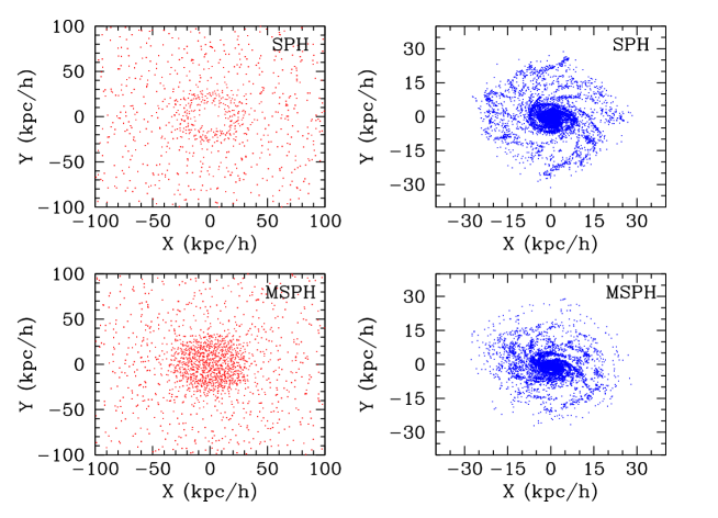
Figure 12: Face-on projections at $t\sim 1.2$ Gyr of 8000 gas particle, cooling only simulations of a collapsing, rotating sphere. The standard SPH simulation is in the upper row with the MSPH simulation below it. The left-hand plots show “hot” particles ($T>10^{5}$K) while the right hand ones show “cold” particles ($T<10^{5}$K and $n_{H}>0.1$ cm^-3). This Figure is taken from Marri & White (2003).

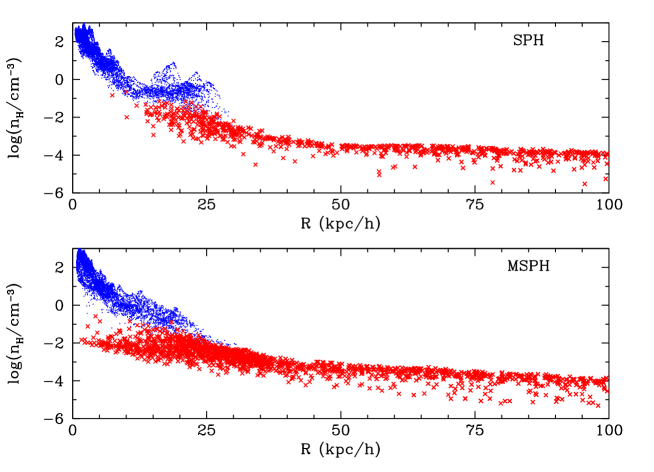
Figure 13: Particle densities as a function of galactocentric distance after $\sim 1.2$ Gyr of evolution in two 8000 gas particle, cooling only simulations of the collapse of a rotating sphere. The upper plot is for an SPH model and the lower for an MSPH model. Gas particles with $T>10^{5}$K are plotted with crosses. This Figure is taken from Marri & White (2003).

6 Feedbacks in the Early Universe

At $z=1000$ the Universe has cooled down to 3000 K and the hydrogen becomes neutral (recombination). Then, at $z\mathrel{\hbox to0.0pt{\lower 3.0pt\hbox{$\sim$}\hss}\raise 2.0pt\hbox{$<$}}20$ the first stars (Population or Pop III stars) form and these gradually photo-ionize the hydrogen in the IGM (reionization). These epoch, witnessing the return of light in the universe after the Big Bang, is usually dubbed as the Cosmic Dawn. At $z<6$, galaxies form most of their stars and grow by merging. Finally at $z<1$, the massive clusters are assembled.

We can distinguish three main feedback types that are fundamentally shaping the universe at cosmic dawn:

1. Stellar Feedback: the process of star formation produces the conditions (destruction of cold gas) such that astration (or even galaxy formation) comes to a halt or is temporarily blocked;

2. Chemical Feedback: massive stars by polluting the ambient gas with heavies, shift the prevailing formation mode toward low mass stars (self-killing population)

3. Radiative Feedback: the process of star formation erases the conditions (molecular formation) necessary to form stars via UV radiation and ionizing photons. Such radiative input heats and ionizes the gas decreasing its ability to produce sources (stars) to further sustain reionization.

In the following we will describe in detail the three feedback types.

6.1 Stellar Feedback

6.1.1 Oxygen in the Low Density IGM

One of the most obvious signatures of stellar feedback is the metal enrichment of the intergalactic medium. If powerful winds are driven by supernova explosions, one would expect to see widespread traces of heavy elements away from their production sites, i.e. galaxies. Schaye et al. (2000) have reported the detection of OVI in the low-density IGM at high redshift. They perform a pixel-by-pixel search for OVI absorption in eight high quality quasar spectra spanning the redshift range $z=2.0-4.5$. At $2\mathrel{\hbox to0.0pt{\lower 3.0pt\hbox{$\sim$}\hss}\raise 2.0pt\hbox{$<$}}z\mathrel{\hbox to0.0pt{\lower 3.0pt\hbox{$\sim$}\hss}\raise 2.0pt\hbox{$<$}}3$ they detect OVI in the form of a positive correlation between the HI Ly$\alpha$ optical depth and the optical depth in the corresponding OVI pixel, down to $\tau_{\rm HI}\sim 0.1$ (underdense regions), that means that metals are far from galaxies (Figure 14). Moreover, the observed narrow widths of metal absorption lines (CIV, SiIV) lines lines imply low temperatures $T_{\rm IGM}\sim{\rm few}\times 10^{4}$ K.

A natural hypothesis would be that the Ly$\alpha$ forest has been enriched by metals ejected by Lyman Break Galaxies at moderate redshift. The density of these objects is $n_{\rm LBG}=0.013$ $h^{3}$ Mpc³. A filling factor of $\sim 1$% is obtained for a shock radius $R_{s}=140$ $h^{-1}$ kpc, that corresponds at $z=3$ ($h=0.5$) to a shock velocity $v_{s}=600$ km s^-1. In this case, we expect a post shock gas temperature larger than $2\times 10^{6}$ K, that is around hundred times what we observed. So the metal pollution must have occurred earlier than redshift 3, resulting in a more uniform distribution and thus enriching vast regions of the intergalactic space. This allows the Ly$\alpha$ forest to be hydrodynamically ‘cold’ at low redshift, as intergalactic baryons have enough time to relax again under the influence of dark matter gravity only (Scannapieco, Ferrara & Madau 2002).

In Figure 15 is shown the thermal history of the IGM as a function of redshift as computed by Madau, Ferrara & Rees (2001). The gas is allowed to interact with the CMB through Compton cooling and either with a time-dependent quasar-ionizing background as computed by Haardt & Madau (1996) or with a time-dependent metagalactic flux of intensity $10^{-22}\,{\rm\,erg\,cm^{-2}\,s^{-1}\,Hz^{-1}\,sr^{-1}}$ at 1 Ryd and power–law spectrum with energy slope $\alpha=1$. The temperature of the medium at $z=9$ has been either computed self-consistently from photoheating or fixed to be in the range $10^{4.6}-10^{5}$ K, as expected in SN-driven bubbles with significant filling factors. The various curves show that the temperature of the IGM at $z=3-4$ will retain little memory of an early era of pregalactic outflows.

The large increase of the IGM temperature at high redshift connected with such an era of pregalactic outflows, causes a larger Jeans mass, thereby preventing gas from accreting efficiently into small dark matter halos (Benson & Madau 2003). For typical preheating energies, the IGM is driven to temperatures just below the virial temperature of halos hosting $L_{\star}$ galaxies. Thus we may expect preheating to have a strong effect on the galaxy luminosity function at $z=0$. Moderate preheating scenarios, with $T_{\rm IGM}\mathrel{\hbox to0.0pt{\lower 3.0pt\hbox{$\sim$}\hss}\raise 2.0pt\hbox{$>$}}10^{5}$ K at $z\sim 10$, are able to flatten the faint-end slope of the luminosity function, producing excellent agreement with observations, without the need for any local strong feedback within galaxies (Figure 16).

Figure 14: IGM Ly$\alpha$-OVI optical depth correlation from the pixel analysis of the spectra of 8 QSOs. Vertical error bars are $1\sigma$ errors, horizontal error bars are smaller than the symbols and are not shown. For $z\mathrel{\hbox to0.0pt{\lower 3.0pt\hbox{$\sim$}\hss}\raise 2.0pt\hbox{$<$}}3$ $\tau_{\rm OVI,app}$ and $\tau_{\rm HI}$ are clearly correlated, down to optical depths as low as $\tau_{\rm HI}\sim 10^{-1}$. A correlation between $\tau_{\rm OVI,app}$ and $\tau_{\rm HI}$ implies that OVI absorption has been detected in the Ly$\alpha$ forest (Schaye et al. 2000).

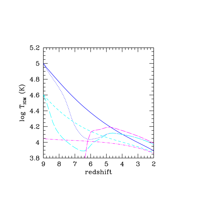
Figure 15: Thermal history of intergalactic gas at the mean density in an Einstein–de Sitter universe with $\Omega_{b}h^{2}=0.019$ and $h=0.5$. Short dash–dotted line: temperature evolution when the only heating source is a constant ultraviolet (CUV) background of intensity $10^{-22}\,{\rm\,erg\,cm^{-2}\,s^{-1}\,Hz^{-1}\,sr^{-1}}$ at 1 Ryd and power–law spectrum with energy slope $\alpha=1$. Long dash–dotted line: same for the time–dependent quasar ionizing background as computed by Haardt & Madau (1996; HM). Short dashed line: heating due to a CUV background but with an initial temperature of $4\times 10^{4}\,$K at $z=9$ as expected from an early era of pregalactic outflows. Long dashed line: same but for a HM background. Solid line: heating due to a CUV background but with an initial temperature of $10^{5}\,$K at $z=9$. Dotted line: same but for a HM background. This Figure is taken from Madau, Ferrara & Rees (2001)

Figure 16: B-band luminosity functions of galaxies at $z=0$, as predicted by the semi-analytic model of Benson et al. (2002). The observational determination of Norberg et al. (2002) is shown as circles. This Figure is taken from Benson & Madau (2003).

6.1.2 Gas Stripping from Neighbor Galaxy Shocks

The formation of a galaxy can be inhibited also by the outflows from neighboring dwarfs as the result of two different mechanisms (Scannapieco et al. 2000). In the “mechanical evaporation” scenario, the gas associated with an overdense region is heated by a shock above its virial temperature. The thermal pressure of the gas then overcomes the dark matter potential and the gas expands out of the halo, preventing galaxy formation. In this case, the cooling time of the collapsing cloud must be shorter than its sound crossing time, otherwise the gas will cool before it expands out of the gravitational well and will continue to collapse.

Alternatively, the gas may be stripped from a collapsing perturbation by a shock from a nearby source. In this case, the momentum of the shock is sufficient to carry with it the gas associated with the neighbor, thus emptying the halo of its baryons and preventing a galaxy from forming.

In principle, outflows can suppress the formation of nearby galaxies both by shock heating/evaporation and by stripping of the baryonic matter from collapsing dark matter halos; in practice, the short cooling times for most dwarf-scale collapsing objects suggest that the baryonic stripping scenario is almost always dominant (Figure 17). This mechanism has the largest impact in forming dwarfs in the $\mathrel{\hbox to0.0pt{\lower 3.0pt\hbox{$\sim$}\hss}\raise 2.0pt\hbox{$<$}}10^{9}M_{\odot}$ range which is sufficiently large to resist photoevaporation by UV radiation, but too small to avoid being swept up by nearby dwarf outflows.

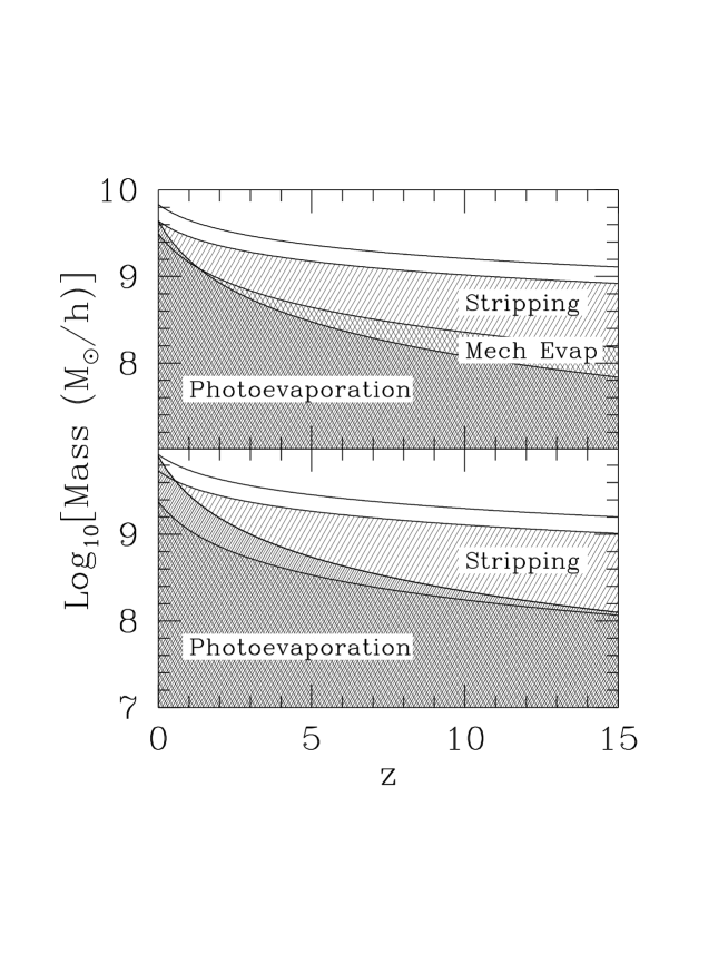
Figure 17: Relevant mass scales for suppression of dwarf galaxy formation. The upper lines are the masses below which halos will be heated beyond their virial temperatures, although cooling prevents mechanical evaporation from occurring for halos with masses above the cross hatched regions. The second highest set of lines, bounding the lightly shaded regions, show the masses below which baryonic stripping is effective. Finally the heavily shaded regions show objects that are susceptible to photoevaporation. The upper panel is a flat CDM model and the lower panel is a flat $\Lambda$CDM model with $\Omega_{0}=0.3$. In all cases $(\epsilon Nh)=5000\Omega_{0}^{-1}$, the overdensity $\delta=\rho/\rho_{0}=2.0$, $\Omega_{b}=0.05$, $h=.65$. Note that photoevaporation affects a larger mass range than mechanical evaporation in the $\Lambda$CDM cosmology. This Figure is taken from Scannapieco et al. (2000)

6.2 Chemical Feedback

Recent studies (Bromm, Coppi & Larson 1999, 2002; Abel, Bryan & Norman 2000; Schneder et al. 2002; Omukai & Inutsuka 2002; Omukai & Palla 2003) have shown that in absence of heavy elements the formation of stars with masses 100 times that of the Sun would have been strongly favored, and that low-mass stars could not have formed before a minimum level of metal enrichment had been reached.

Bromm et al. (2001) have studied the effect of the metallicity on the evolution of the gas in a collapsing dark matter mini-halo, simulating an isolated 3$\sigma$ peak of mass $2\times 10^{6}\;M_{\odot}$ that collapse at $z\sim 30$, using smoothed particle hydrodynamics. The gas has a supposed level of pre-enrichment of either $Z=10^{-4}\;Z_{\odot}$ of $10^{-3}\;Z_{\odot}$. The H₂ is assumed to be radiatively destroyed by the presence of a soft UV background. Moreover Bromm et al. (2001) do not consider the presence of molecules or dust.

The evolution proceeds very differently for the two cases. The gas in the lower metallicity case fails to undergo continued collapse and fragmentation, remaining in the post-virialization, pressure-supported state in a roughly spherical configuration. The final result is likely to be the formation of a single very massive ($\sim 10^{3}-10^{4}\;M_{\odot}$) object (Figure 18). On the other hand (Figure 19), the gas in the higher metallicity case can cool efficiently and collapse into a disk-like configuration. The disk material is gravitational unstable and fragments into a large number of high density clumps, that are the seeds of low mass stars. So, they conclude that there exists a critical metallicity $Z_{crit}$ at which the transition from the formation of high mass objects to a low-mass star formation mode, as we observe at present, occurs. In the following we refer to Pop III stars in the mass range 100-600 $M_{\odot}$ forming out of the collapse of $Z<Z_{crit}$ gas clouds.

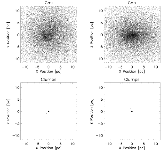
Figure 18: Simulation of a collapsing dark matter halo with mean metallicity of $Z=10^{-4}\;Z_{\odot}$. Morphology at $z=22.7$. Top row: the remaining gas in the diffuse phase. Bottom row: distribution of clumps. Dot sizes are proportional to the mass of the clumps. Left panels: face-on view. Right panels: edge-on view. The box size is 30 pc. It can be seen that no fragmentation occurs. This Figure is taken from Bromm et al. (2001).

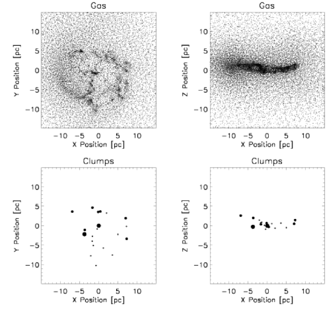
Figure 19: Simulation of a collapsing dark matter halo with mean metallicity of $Z=10^{-3}\;Z_{\odot}$. Morphology at $z=28$. The convention of Figure 18 is adopted for the row and columns. It can be seen that the gas has undergone vigorous fragmentation. This Figure is taken from Bromm et al. (2001)

More recently, Schneider et al. (2002) have investigated the problem more in detail including the cooling due to H₂, molecular, and dust, using the model of Omukai (2001). The gas within the dark matter halo is given an initial temperature of 100 K, and the subsequent thermal and chemical evolution of the gravitationally collapsing cloud is followed numerically until a central protostellar core forms. The results for different metallicities are summarized in Figure 20, showing the temperature and adiabatic index evolution as a function of the hydrogen number density of protostellar clouds for different metallicity ($Z=0,10^{-6},10^{-4},10^{-2},1\;Z_{\odot}$). The necessary conditions to stop fragmentation and start gravitational contraction within each clump are that cooling becomes inefficient, and the Jeans mass of the fragments does not decrease any further, thus favoring fragmentation into sub-clumps. This condition depends somewhat on the geometry of the fragments, and translates into $\gamma>4/3$ ($\gamma>1$) for spherical (filamentary) clumps, where $\gamma$ is the adiabatic index defined as $T\propto n^{\gamma-1}$.

For a metal-free gas, the only efficient coolant is molecular hydrogen. Cooling due to molecular line emission becomes inefficient at densities above $n>10^{3}\,\mbox{cm}^{-3}$, and fragmentation stops when the minimum fragment mass is of order $10^{3}-10^{4}\;M_{\odot}$. Clouds with mean metallicity $Z=10^{-6}\;Z_{\odot}$ follow the same evolution as that of the gas with primordial composition in the $(n,T)$ plane. For metallicities larger than $10^{-4}\;Z_{\odot}$ the fragmentation proceeds further until the density is $\sim 10^{13}$ cm^-3 and the corresponding Jeans mass is of the order $10^{-2}\;M_{\odot}$. Schneider et al. (2002) concluded that the critical metallicity locates in the range $10^{-6}-10^{-4}\;Z_{\odot}$.

According to the scenario proposed above, the first stars that form out of gas of primordial composition tend to be very massive, with masses $\sim 10^{2}-10^{3}\;M_{\odot}$. It is only when metals change the composition of the gas that further fragmentation occurs, producing stars with significantly lower masses. A series of numerical studies (Heger & Woosley 2001; Fryer et al. 2001; Umeda & Nomoto 2002) have investigated the nucleosynthesis and final state of metal-free massive stars. Heger & Woosley (2001) delineate three mass ranges characterized by distinct evolutionary paths:

1. $M_{\star}\mathrel{\hbox to0.0pt{\lower 3.0pt\hbox{$\sim$}\hss}\raise 2.0pt\hbox{$>$}}260\;M_{\odot}$. – The nuclear energy released from the collapse of stars in this mass range is insufficient to reverse the implosion. The final result is a very massive black hole (VMBH) locking up all heavy elements produced.

2. $140\;M_{\odot}\mathrel{\hbox to0.0pt{\lower 3.0pt\hbox{$\sim$}\hss}\raise 2.0pt\hbox{$<$}}M_{\star}\mathrel{\hbox to0.0pt{\lower 3.0pt\hbox{$\sim$}\hss}\raise 2.0pt\hbox{$<$}}260\;M_{\odot}$. – The mass regime of the pair-unstable supernovae (SN_γγ). Precollapse winds and pulsations result in little mass loss; the star implodes to a maximum temperature that depends on its mass and then explodes, leaving no remnant. The explosion expels metals into the surrounding ambient ISM.

3. $30\;M_{\odot}\mathrel{\hbox to0.0pt{\lower 3.0pt\hbox{$\sim$}\hss}\raise 2.0pt\hbox{$<$}}M_{\star}\mathrel{\hbox to0.0pt{\lower 3.0pt\hbox{$\sim$}\hss}\raise 2.0pt\hbox{$<$}}140\;M_{\odot}$. – Black hole formation is the most likely outcome, because either a successful outgoing shock fails to occur or the shock is so weak that the fallback converts the neutron star remnant into a black hole (Fryer 1999)

Stars that form in the mass ranges 1 and 3 above fail to eject most of their heavy elements. If the first stars have masses in excess of 260 $M_{\odot}$, they invariably end their lives as VMBHs and do not release any of their synthesized heavy elements. However, as long as the gas remains metal free, the subsequent generations of stars will continue to be top-heavy. This ‘star formation conundrum’ can be solved only if a fraction $f_{\gamma\gamma}$ of the first generation of massive stars are in the SN_γγ range and enrich the gas with heavy elements up to a mean metallicity of $Z\geq 10^{-5\pm 1}\;Z_{\odot}$.

Schneider et al. (2002) computed the transition redshift $z_{f}$ at which the mean metallicity is $10^{-4}\;Z_{\odot}$ for various values of $f_{\gamma\gamma}$. The results are plotted in Figure 21 along with the corresponding critical density $\Omega_{VMBH}$ contributed by the VMBHs formed. In order to set some limits on $f_{\gamma\gamma}$, we have to compare the predicted critical density of VMBH remnants to present observational data. This depends on the assumptions about the fate of these VMBHs at late times.

Under the hypothesis that all VMBHs have, during the course of galaxy mergers, been used to build up the supermassive black holes (SMBHs) detected today so that $\Omega_{VMBH}=\Omega_{SMBH}$, from the top panel of Figure 21 we can derive $f_{\gamma\gamma}\simeq 0.06$ and $z_{f}\simeq 18.5$.

Figure 20: Top: Evolution of the temperature as a function of the hydrogen number density of protostellar clouds with the same initial gas temperature but varying the metallicities $Z=(0,10^{-6},10^{-4},10^{-2},1)\;Z_{\odot}$ ($Z$ increasing from top to bottom curves). The dashed lines correspond to the constant Jeans mass for spherical clumps; open circles indicates the points where fragmentation stops; filled circles mark the formation of hydrostatic cores. Bottom: The adiabatic index $\gamma$ as a function of the hydrogen number density for the curves shown in the top panel. Dotted (dashed) lines correspond to $\gamma=1$ ($\gamma=4/3$); open and filled circles as above. This Figure is taken from Schneider et al. (2002).

At the other extreme, wherein the assembled SMBHs in galactic centers have formed primarily via accretion and are unrelated to VMBHs, two possibilities can be distinguish: (1) VMBHs would still be in the process of spiraling into the center of galaxies because of dynamical friction but are unlikely to have reached the center within a Hubble time because of the long dynamical friction timescale (Madau & Rees 2001), or, (2) VMBHs contribute the entire baryonic dark matter in galactic halos. In case (1) some fraction of these VMBHs might appear as off-center accreting sources that show up in hard X-ray wave band. In fact, ROSAT and Chandra have detected such objects. Using the contribution to $\Omega$ from X-ray-bright, off-center ROSAT sources as a limit for the density of VMBHs, from the lower dashed line in the bottom panel of Figure 21 $f_{\gamma\gamma}$ has to be nearly unity and $z_{f}\mathrel{\hbox to0.0pt{\lower 3.0pt\hbox{$\sim$}\hss}\raise 2.0pt\hbox{$>$}}22.1$. In case (2), assuming that the baryonic dark matter in galaxy halos is entirely contributed by VMBH (upper dashed line in the bottom panel of Figure 21), $f_{\gamma\gamma}\simeq 3.15\times 10^{-5}$ and $z_{f}\mathrel{\hbox to0.0pt{\lower 3.0pt\hbox{$\sim$}\hss}\raise 2.0pt\hbox{$>$}}5.4$. Therefore the case in which SMBHs are unrelated to VMBHs, only weak limits for $f_{\gamma\gamma}$ and $z_{f}$ can be obtained. Although the actual data do not allow us at present to strongly constrain these two quantities, they provide interesting bounds on the proposed scenario.

We have seen that there exists a critical metallicity $Z_{cr}=10^{5\pm 1}\;Z_{\odot}$ (Schneider et al. 2002; 2003) at which we expect the transition between a top-heavy and a normal Salpeter-like IMF. One point that might have important observational consequences is the fact that cosmic metal enrichment has proceeded very inhomogeneously (Scannapieco, Ferrara & Madau 2002; Furlanetto & Loeb 2003; Marri et al. 2003), with regions close to star formation sites rapidly becoming metal-polluted and overshooting $Z_{cr}$, and others remaining essentially metal-free. Thus, the two modes of star formation, Pop III and normal, must have been active at the same time and possibly down to relatively low redshifts, opening up the possibility of detecting Pop III stars.

Scannapieco, Schneider & Ferrara (2003) have studied using an analytic model of inhomogeneous structure formation, the evolution of Pop III objects as a function of the star formation efficiency, IMF, and efficiency of outflow generation. They parametrized the chemical feedback through a single quantity, $E_{g}$, which represents the kinetic energy input per unit gas mass of outflows from Pop III galaxies. This quantity is related to the number of exploding Pop III stars and therefore encodes the dependence on the assumed IMF. For all values of the feedback parameter, $E_{g}$, Scannapieco et al. (2003) found that, while the peak of Pop III star formation occurs at $z\sim 10$, such stars continue to contribute appreciably to the star formation rate density at much lower redshift, even though the mean IGM metallicity has moved well past the critical transition metallicity. This finding has

Figure 21: Top-heavy to normal IMF transition redshift, $z_{f}$, as a function of SN_γγ progenitor mass fraction and the mass density contributed by VMBHs, $\Omega_{VMBH}$. Top: The computed critical density of VMBH remnants is compared to the observed values for SMBHs (upper dashed line). Bottom: The computed critical density of VMBH remnants is compared to the contribution to $\Omega$ from the X-ray-bright, off-center ROSAT sources (lower dashed line) and to the abundance predicted assuming that the baryonic dark matter in galaxy halos is entirely contributed by VMBHs (upper dashed line). The observations on $\Omega_{VMBH}$ constrain the value of $f_{\gamma\gamma}$. For a given $f_{\gamma\gamma}$, the corresponding value for the transition redshift can be inferred by the $z_{f}$ curve. This Figure is taken from Schneider et al. (2002).

important implications for the development of efficient strategies for the detection of Pop III stars in primeval galaxies. At any given redshift, a fraction of the observed objects have a metal content that is low enough to allow the preferential formation of Pop III stars. As metal-free stars are powerful Ly$\alpha$ emitters (Tumlinson, Giroux & Shull 2001; Schaerer 2003), it is natural to use this indicator as a first step in any search for primordial objects. Scannapieco et al. (2003) derived the probability that a given high-redshift Ly$\alpha$ detection is due to a cluster of Pop III stars. In Figure 22 the isocontours in the Ly$\alpha$ luminosity-redshift plane are shown, indicating this probability for various feedback efficiencies $E_{g}^{III}$. We see that Pop III objects populate a well-defined region, whose extent is governed by the feedback strength. Above the typical flux threshold, Ly$\alpha$ emitters are potentially detectable at all redshifts beyond 5. Furthermore, the fraction of Pop III objects increases with redshift, independently of $E_{g}^{III}$. For the fiducial case, $E_{g}^{III}=10^{-3}$, the fraction is only a few percent at $z=4$ but increases to approximately 15% by $z=6$. So, the Ly$\alpha$ emission from already observed high-$z$ sources can indeed be due to Pop III objects, if such stars were biased toward high masses. Hence collecting large data samples to increase the statistical leverage may be crucial for detecting the elusive first stars.

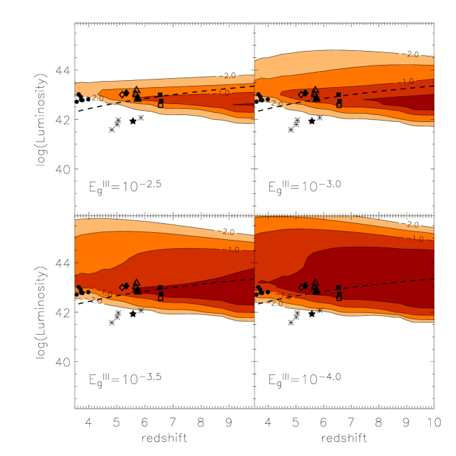
Figure 22: Fraction of PopIII objects as a function of Ly$\alpha$ luminosity and redshift. Isocontours of fractions $\geq 10^{-2},10^{-1.5},10^{-1}$ and $10^{0.5}$ are shown. Burst-mode star formation with a $f_{\star}^{II}=f_{\star}^{III}=0.1$ is assumed for all objects. In the PopIII case, a lower cutoff mass of $50M_{\odot}$ is assumed. Each panel is labeled by the assumed $E_{g}^{III}$ value. For reference, the dashed line gives the luminosity corresponding to an observed flux of $1.5\times 10^{-17}$ ergs cm^-2 s^-1, and the various points correspond to observed galaxies. The filled diamond is from Dey et al. (1998), the filled triangle is from Hu et al. (1999), the filled star is from Ellis et al. (2001), the open diamond is from Dawson et al. (2002), the open square is from Hu et al. (2002), the asterisks are from Lehnert & Bremer (2003), the open triangles are from Rhoads et al. (2003), the filled circles are from Fujita et al. (2003), and the filled squares are from Kodaira et al. (2003). The curves have been extended slightly past $z=4$ for comparison with the Fujita et al. (2003) data-set. This Figure is taken from Scannapieco, Schneider & Ferrara (2003).

6.3 Radiative Feedback and Reionization

Before metals are produced, the primary molecule which acquires sufficient abundance to affect the thermal state of the pristine cosmic gas is molecular hydrogen, H₂. The main reaction able to produce molecular hydrogen are (Abel et al. 1997)

$$\rm H\ \ \ \ +\ \ e^{-}\ \rightarrow \ \ {\rm H^{-}}\ \ +\ \ h\nu,$$ (54)

$$\rm H^{-}\ \ +\ \ H\ \ \rightarrow \ \ \rm H_{2}\ \ \ +\ \ e^{-},$$ (55)

and

$$\rm H^{+}\ \ +\ \ H\ \ \rightarrow \ \ {\rm H_{2}^{+}}\ \ +\ \ h\nu,$$ (56)

$$\rm H_{2}^{+}\ \ +\ \ H\ \ \rightarrow \ \ \rm H_{2}\ \ +\ \ H^{+},$$ (57)

In objects with baryonic masses $\mathrel{\hbox to0.0pt{\lower 3.0pt\hbox{$\sim$}\hss}\raise 2.0pt\hbox{$>$}}3\times 10^{4}\;M_{\odot}$, gravity dominates and results in the bottom-up hierarchy of structure formation characteristic of CDM cosmologies; at lower masses, gas pressure delays the collapse. The first objects to collapse are those at the mass scale that separates these two regimes. Such objects have a virial temperature of several hundred degrees and can fragment into stars only through molecular cooling (Tegmark et al. 1997). In other words, there are two independent minimum mass thresholds for star formation: the Jeans mass (related to accretion) and the cooling mass. For the very first objects, the cooling threshold is somewhat higher and sets a lower limit on the halo mass of $\sim 5\times 10^{4}\;M_{\odot}$ at $z\sim 20$.

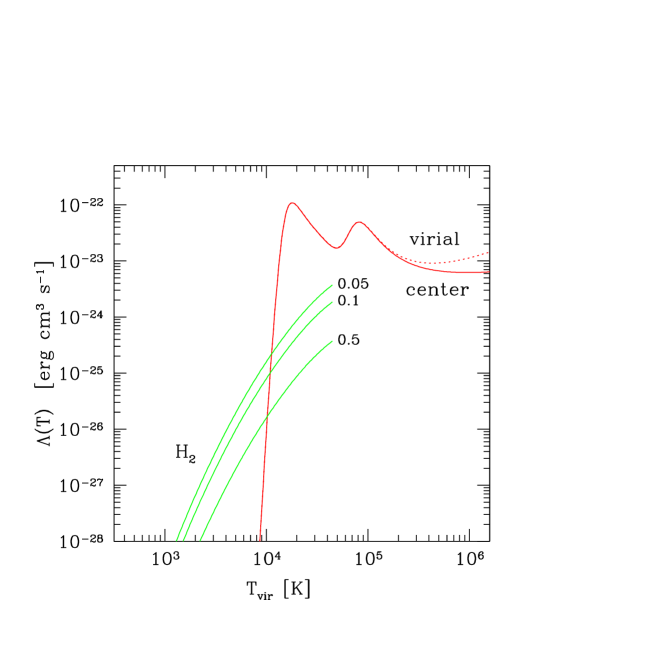
Figure 23: Equilibrium cooling curve at the center (solid lines) and virial radius (dashed line) of an isothermal halo at $z=9$, as a function of virial temperature $T_{vir}$, and in the absence of a photoionizing background (i.e. prior to the reionization epoch). The halo has an assumed baryonic mass fraction of $\Omega_{b}=0.019h^{-2}$. The gas density dependence of the cooling function at high temperatures is due to Compton cooling off comic microwave background photons. The labeled curves extending to low temperatures show the contribution due to H₂ for three assumed values of the metagalactic flux in the Lyman-Werner bands, $4\pi J_{\rm LW}$ (in units of $10^{-21}\,{\rm\,erg\,cm^{-2}\,s^{-1}\,Hz^{-1}}$). This Figure is taken from Madau, Ferrara & Rees (2001).

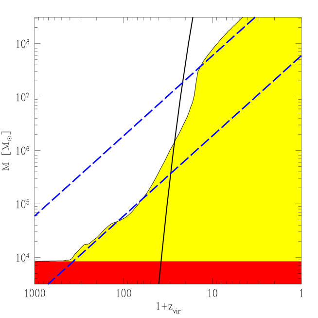
Figure 24: The minimum mass needed to collapse. The function $M_{c}(z_{vir})$ is plotted as a function on virialization redshift for standard CDM ($\Omega=1$, $\Omega_{b}=0.06$, $h=0.5$). Only lumps whose parameters $(z_{vir},M)$ lie above the shaded area can collapse and form luminous objects. The dashed straight lines corresponding to $T_{vir}=10^{4}$ K and $T_{vir}=10^{3}$ K are shown for comparison (dashed). The dark-shaded region is that in which no radiative cooling mechanism whatsoever could help collapse, since $T_{vir}$ would be lower than the CMB temperature. The solid line corresponds to $3-\sigma$ peaks in standard CDM, normalized to $\sigma_{8}=0.7$, so such objects with baryonic mass $\Omega_{b}\times 2\times 10^{6}\;M_{\odot}\sim 10^{5}\;M_{\odot}$ can form at $z=30$. This figure is taken from Tegmark et al. (1997).

As the first stars form, their photons in the energy range 11.26-13.6 eV are able to penetrate the gas and photodissociate H₂ molecules both in the IGM and in the nearest collapsing structures, if they can propagate that far from their source. Thus, the existence of an UV background below the Lyman limit due to Pop III objects, capable of dissociating the H₂, could deeply influence subsequent small structure formation.

Ciardi, Ferrara & Abel (2000) have shown that the UV flux from these objects results in a soft (Lyman – Werner band) UV background (SUVB), $J_{LW}$, whose intensity (and hence radiative feedback efficiency) depends on redshift. At high redshift the radiative feedback can be induced also by the direct dissociating flux from a nearby object. In practice, two different situations can occur: i) the collapsing object is outside the dissociated spheres produced by pre-existing objects: then its formation could be affected only by the SUVB ($J_{LW,b}$), as by construction the direct flux ($J_{LW,d}$) can only dissociate molecular hydrogen inside this region on time scales shorter than the Hubble time; ii) the collapsing object is located inside the dissociation sphere of a previously collapsed object: the actual dissociating flux in this case is essentially given by $J_{LW,max}=(J_{LW,b}+J_{LW,d})$. It is thus assumed that, given a forming Pop III, if the incident dissociating flux ($J_{LW,b}$ in the former case, $J_{LW,max}$ in the latter) is higher than the minimum flux required for negative feedback ($J_{s}$), the collapse of the object is halted. This implies the existence of a population of ”dark objects” which were not able to produce stars and, hence, light.

To assess the minimum flux required at each redshift to drive the radiative feedback Ciardi et al. (2000) have performed non-equilibrium multifrequency radiative transfer calculations for a stellar spectrum (assuming a metallicity $Z=10^{-4}$) impinging onto a homogeneous gas layer, and studied the evolution of the following nine species: H, H^-, H⁺, He, He⁺, He⁺⁺, H₂, H${}_{2}^{+}$ and free electrons for a free fall time. We can then define the minimum total mass required for an object to self-shield from an external flux of intensity $J_{s,0}$ at the Lyman limit, as $M_{sh}=(4/3)\,\pi\langle\rho_{h}\rangle R_{sh}^{3}$, where $\langle\rho_{h}\rangle$ is the mean dark matter density of the halo in which the gas collapses; $R_{sh}$ is the shielding radius beyond which molecular hydrogen is not photodissociated and allowing the collapse to take place on a free-fall time scale.

Values of $M_{sh}$ for different values of $J_{s,0}$ have been obtained at various redshifts (see Figure 25). Protogalaxies with masses above $M_{H}$ for which cooling is predominantly contributed by Ly$\alpha$ line are not affected by the radiative feedback studied here. The collapse of very small objects with mass $<M_{crit}$ is on the other hand not possible since the cooling time is longer than the Hubble time. Thus radiative feedback is important in the mass range $10^{6}-10^{8}M_{\odot}$, depending on redshift. In order for the negative feedback to be effective, fluxes of the order of $10^{-24}-10^{-23}$erg s^-1 cm^-2 Hz^-1 sr^-1 are required. These fluxes are typically produced by a Pop III with baryonic mass $10^{5}M_{b,5}M_{\odot}$ at distances closer than $\simeq 21-7\times M_{b,5}^{1/2}$ kpc for the two above flux values, respectively, while the SUVB can reach an intensity in the above range only after $z\approx 15$. This suggests that at high $z$ negative feedback is driven primarily by the direct irradiation from neighbor objects in regions of intense clustering, while only for $z\leq 15$ the SUVB becomes dominant.

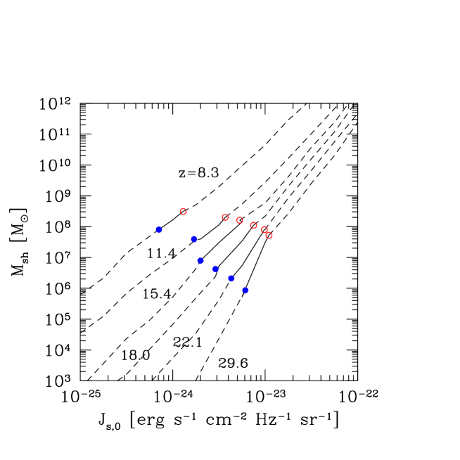
Figure 25: Minimum total mass for self-shielding from an external incident flux with intensity $J_{s,0}$ at the Lyman limit. The curves are for different redshift: from the top to the bottom $z=$8.3, 11.4, 15.4, 18.0, 22.1, 29.6. Circles show the value of $M_{H}$ (open) and $M_{crit}$ (filled). Radiative feedback works only in the solid portions of the curves. This Figure is taken from Ciardi et al. (2000)

Figure 26 illustrates all possible evolutionary tracks and final fates of primordial objects, together with the mass scales determined by the various physical processes and feedbacks. There are four critical mass scales in the problem: (i) $M_{crit}$, the minimum mass for an object to be able to cool in a Hubble time; (ii) $M_{H}$, the critical mass for which hydrogen Ly$\alpha$ line cooling is dominant; (iii) $M_{sh}$, the characteristic mass above which the object is self-shielded, and (iv) $M_{by}$ the characteristic mass for stellar feedback, below which blowaway can not be avoided. Starting from a virialized dark matter halo, condition (i) produces the first branching, and objects failing to satisfy it will not collapse and form only a negligible amount of stars. In the following, we will refer to these objects as dark objects. Protogalaxies with masses in the range $M_{crit}<M<M_{H}$ are then subject to the effect of radiative feedback, which could either impede the collapse of those of them with mass $M<M_{sh}$, thus contributing to the class of dark objects, or allow the collapse of the remaining ones ($M>M_{sh}$) to join those with $M>M_{H}$ in the class of luminous objects. This is the class of objects that convert a considerable fraction of their baryons in stars. Stellar feedback causes the final bifurcation by inducing a blowaway of the baryons contained in luminous objects with mass $M<M_{by}$; this separates the class in two subclasses, namely ”normal” galaxies (although of masses comparable to present day dwarfs) that we dub gaseous galaxies and tiny stellar aggregates with negligible traces (if any) of gas to which consequently we will refer to as naked stellar clusters.

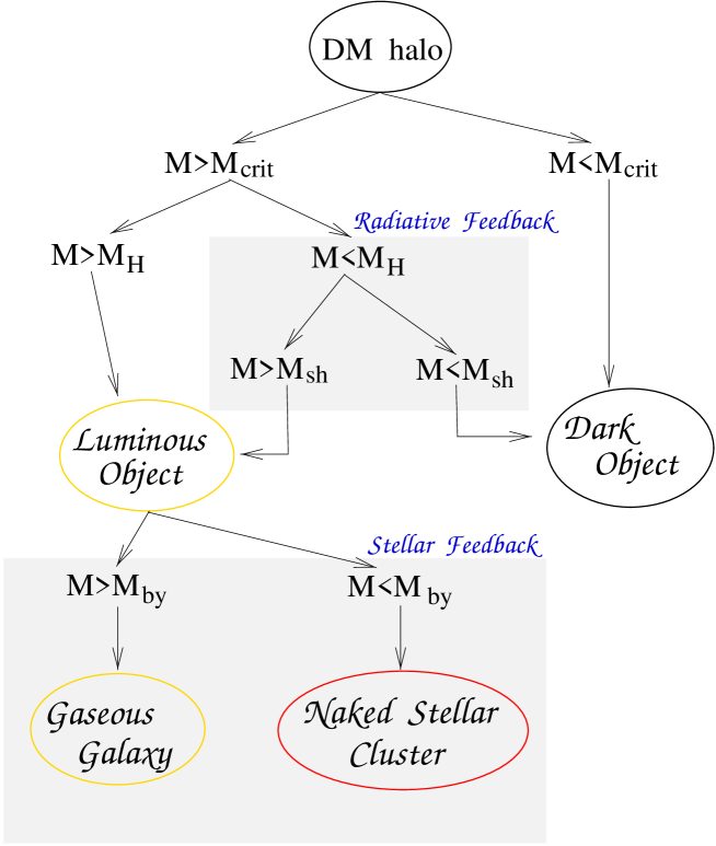
Figure 26: Possible evolutionary tracks of objects as determined by the processes and feedbacks included in the model. See text. This figure is taken from Ciardi et al. (2000)

The relative numbers of these objects are shown in Figure 27. The straight lines represent, from the top to the bottom, the number of dark matter halos, dark objects, naked stellar clusters and gaseous galaxies, respectively. The dotted curve represents the number of luminous objects with large enough mass ($M>M_{H}$) to make the H line cooling efficient and become insensitive to the negative feedback. We remind that the naked stellar clusters are the luminous objects with $M<M_{by}$, while the gaseous galaxies are the ones with $M>M_{by}$; thus, the number of luminous objects present at a certain redshift is given by the sum of naked stellar clusters and gaseous galaxies. We first notice that the majority of the luminous objects that are able to form at high redshift will experience blowaway, becoming naked stellar clusters, while only a minor fraction, and only at $z\mathrel{\hbox to0.0pt{\lower 3.0pt\hbox{$\sim$}\hss}\raise 2.0pt\hbox{$<$}}$15, when larger objects start to form, will survive and become gaseous galaxies. An always increasing number of luminous objects is forming with decreasing redshift, until $z\sim 15$, where a flattening is seen. This is due to the fact that the dark matter halo mass function is still dominated by small mass objects, but a large fraction of them cannot form due to the following combined effects: i) toward lower redshift the critical mass for the collapse ($M_{crit}$) increases and fewer objects satisfy the condition $M>M_{crit}$; ii) the radiative feedback due to either the direct dissociating flux or the SUVB increases at low redshift as the SUVB intensity reaches values significant for the negative feedback effect. When the number of luminous objects becomes dominated by objects with $M>M_{H}$, by $z\sim 10$ the population of luminous objects grows again, basically because their formation is now unaffected by negative radiative feedback. A steadily increasing number of objects is prevented from forming stars and remains dark; this population is about $\sim 99$% of the total population of dark matter halos at $z\sim 8$. This is also due to the combined effect of points i) and ii) mentioned above. This population of halos which have failed to produce stars could be identified with the low mass tail distribution of the dark galaxies that reveal their presence through gravitational lensing of quasars. It has been argued that this population of dark galaxies outnumbers normal galaxies by a substantial amount, and Figure 27 supports this view.

Figure 27: Number evolution of different objects in the simulation box. This Figure is taken from Ciardi et al. (2000)

6.3.1 Escape of Ionizing Photons

One crucial point to understand cosmic reionization is to determine the fraction of ionizing photons that can escape from their parent galaxy. By solving the time-dependent radiation transfer problem of stellar radiation through evolving superbubbles within a smoothly varying H I distribution, Dove et al. (2000) have estimated the fraction of ionizing photons emitted by OB associations that escapes the H I disk of our Galaxy into the halo and intergalactic medium (IGM). They considered both coeval star-formation and a Gaussian star-formation history with a time spread $\sigma_{t}=2$ Myr; the calculations are performed both a uniform H I distribution and a two-phase (cloud/intercloud) model, with a negligible filling factor of hot gas. The shells of the expanding superbubbles quickly trap or attenuate the ionizing flux, so that most of the escaping radiation escapes shortly after the formation of the superbubble. Superbubbles of large associations can blow out of the H I disk and form dynamic chimneys, which allow the ionizing radiation to escape the H I disk directly. However, blowout occurs when the ionizing photon luminosity has dropped well below the association’s maximum luminosity. For the coeval star-formation history, the total fraction of Lyman Continuum photons that escape both sides of the disk in the solar vicinity is $\langle f_{esc}\rangle\simeq 0.15\pm 0.05$ (Figure 28). For the Gaussian star formation history, $\langle f_{esc}\rangle\simeq 0.06\pm 0.03$.

Figure 28: Photon luminosity emitted by a single OB association (solid line) and the luminosity of photons escaping each side of the H I disk (dashed line) for coeval star-formation. Also shown is the fraction of photons emitted that escape, $\eta_{esc}(N_{T},t)=S_{esc}(t)/S(t)$. Here, $Z_{tr}=2\sigma_{h}$, the cavity height is $Z_{cy}=4\sigma_{h}$, and $\beta=1$. The I-front is trapped within the shell during the time interval where $\eta_{esc}=0$. After blowout, $\eta_{esc}$ suddenly increases even though the photon luminosity of the association is relatively low at these times. Case with $N_{\star}=200$. This Figure is taken from Dove et al. (2000)

Bianchi, Cristiani & Kim (2001) derived the HI-ionizing background, resulting from the integrated contribution of QSOs and galaxies, taking into account the opacity of the intervening IGM. They have modeled the IGM with pure-absorbing clouds, with a distribution in column density of neutral hydrogen, $N_{\rm HI}$, and redshift, $z$, derived from recent observations of the Ly$\alpha$ forest (Kim et al. 2002) and from Lyman Limit systems. The QSOs emissivity has been derived from the recent fits of Boyle et al. (2000), while the stellar population synthesis model of Bruzual & Charlot (2003) and a star-formation history from UV observations for the galaxy emissivity. Due to the present uncertainties in models and observations, three values for the fraction of ionizing photons that can escape a galaxy interstellar medium, $f_{esc}$= 0.05, 0.1 and 0.4, as suggested by local and high-$z$ UV observations of galaxies, respectively, are used.

In Figure 29 is shown the modeled UV background, $J(\nu,z)$, at the Lyman limit as a function of redshift (solid lines) for the flat universe with $\Omega_{m}$=1. The total background is shown as the sum of the QSO contribution (the same in each model; dotted line) and the galaxy contribution (scaled with $f_{esc}$; dashed lines).

At high redshift, the value of the UV background is constrained by the analysis of the proximity effect, i.e. the decrease in the number of intervening absorption lines that is observed in a QSO spectrum when approaching the QSO’s redshift (Bajtlik et al. 1988). Using high resolution spectra, Giallongo et al. (1996) derived $J(912$Å$)=5.0_{-1}^{+2.5}\times 10^{-22}\;\mathrm{erg\;cm^{-2}\;s^{-1}\;Hz^{-1}\;sr^{-1}}$ for $1.7<z<4.1$ (see also Giallongo et al. 1999). Larger values are obtained (same units) by Cooke et al. (1997), $J(912$Å$)=1.0_{-0.3}^{+0.5}\times 10^{-21}$ for $2.0<z<4.5$ and by a recent re-analysis of moderate resolution spectra by Scott et al. (2000) who found $J(912$Å$)=7.0_{-4.4}^{+3.4}\cdot 10^{-22}$ in the same redshift range. These measurements are shown in Figure 29 with a shaded area: the spread of the measurements obtained with different methods and data gives an idea of the uncertainties associated with the study of the proximity effect. Several models can produce a value of $J(912$Å$)$ compatible with one of the measurements from the proximity effect at $z\sim 3$ shown in Figure 29, from a simple QSO-dominated background to models with $f_{esc}\sim 0.2$, leading to a limit of $f_{esc}\mathrel{\hbox to0.0pt{\lower 3.0pt\hbox{$\sim$}\hss}\raise 2.0pt\hbox{$<$}}20$%.

Figure 29: UV background at $\lambda=912$Å for the models with $f_{esc}$=0.05, 0.1 and 0.4 (solid lines), in a flat $\Omega_{m}=1$ universe. Also shown are the separate contribution of the QSOs (dotted line) and of the galaxies (dashed lines, each corresponding to a value of $f_{esc}$). The shaded area refer to the Lyman limit UV background estimated from the proximity effect (Giallongo et al. 1996; Cooke et al. 1997; Scott et al. 2000). The arrow shows an upper limit for the local ionizing background (Vogel et al. 1995). The datapoint at $z=3$ is derived from a composite spectrum of Lyman-break galaxies (Steidel et al. 2001). The models and the datapoint of Steidel et al. (2001) have been multiplied by a $z$-dependent factor, to take into account the cloud emission. This Figure is taken from Bianchi et al. (2001)

6.3.2 Cosmological Ionization Fronts

The radiative transfer equation in cosmology describes the time evolution of the specific intensity $I_{\nu}=I(t,x,\omega,\nu)$ of a diffuse radiation field (Ciardi, Ferrara & Abel 2000):

$$\frac{1}{c}\frac{\partial I_{\nu}}{\partial t}+\frac{\hat{n}\cdot\nabla I_{\nu}}{a_{em}}-\frac{H(t)}{c}\left[v\frac{\partial I_{\nu}}{\partial\nu}-3I_{\nu}\right]=\eta_{\nu}-\chi I_{\nu},$$ (58)

where $c$ is the speed of light, $\chi$ is the continuum absorption coefficient per unit length along the line of sight, and $\eta_{\nu}$ is the proper space averaged volume emissivity.

If massive stars form in Pop III objects, their photons with $h\nu>13.6$ eV create a cosmological HII region in the surrounding IGM. Its radius, $R_{i}$, can be estimated by solving the following standard equation for the evolution of the ionization front:

$$\frac{dR_{i}}{dt}-HR_{i}=\frac{1}{4\pi n_{H}R_{i}^{2}}\left[S_{i}(0)-\frac{4}{3}\pi R_{i}^{3}n_{H}^{2}\alpha^{(2)}\right];$$ (59)

note that ionization equilibrium is implicitly assumed. $H$ is the Hubble constant, $S_{i}(0)$ is the ionizing photon rate, $n_{H}$ is the IGM hydrogen number density and $\alpha^{(2)}$ is the hydrogen recombination rate to levels $\geq 2$. For $aR\gg c/H$ the cosmological expansion term $HR_{i}$ can be safely neglected. In its full form equation (59) must be solved numerically. However, if steady-state is assumed ($dR_{i}/dt\simeq 0$), then $R_{i}$ is approximately equal to the Stromgren radius $R_{s}(z)=[(3dN_{\gamma}/dt)/(4\pi\alpha_{2}n_{H}^{2}(z))]^{1/3}$:

$$R_{i}\simeq R_{s}=0.05(\Omega_{b}h^{2})^{-2/3}(1+z)_{30}^{-2}S_{47}^{1/3}{\rm kpc},$$ (60)

where $S_{47}=S_{i}(0)/10^{47}{\rm s^{-1}}$. The approximate expression for $S_{i}(0)$ is $\simeq 1.2\times 10^{48}f_{b}M_{6}$ s^-1 when a 20% escape fraction for ionizing photons is assumed and $f_{b}$ is the fraction of baryon that is able to cool and become available to form stars. In general $R_{s}$ represents an upper limit for $R_{i}$, since the ionization front completely fills the time-varying Stromgren radius only at very high redshift, $z\simeq 100$.

6.3.3 Reionization after WMAP

The WMAP satellite has detected an excess in the CMB TE cross-power spectrum on large angular scales ($l<7$) indicating an optical depth to the CMB last scattering surface of $\tau_{e}=0.17\pm 0.04$ (Kogut et al. 2003). The reionization of the universe must therefore have begun at relatively high redshift. Ciardi, Ferrara & White (2003) have studied the reionization process using supercomputer simulations of a large and representative region of a universe which has cosmological parameters consistent with the WMAP results. The simulation follow both the radiative transfer of ionizing photons and the formation and evolution of the galaxy population which produces them.

They have shown that the WMAP measured optical depth to electron scattering is easily reproduced by a model in which reionization is caused by the first stars in galaxies with total masses of a few $\times 10^{9}\;M_{\odot}$. Moreover, the first stars are ‘normal objects’, i.e. their mass is in the range 1-50 $M_{\odot}$, but metal-free. Among the different model explored, the ‘best’ WMAP value for $\tau_{e}$ is matched assuming a moderately top-heavy IMF (Larson IMF with $M_{c}=5\;M_{\odot}$) and an escape fraction of 20%. A Salpeter IMF with the same escape fraction gives $\tau_{e}=0.132$, which is still within the WMAP 68% confidence range. Decreasing $f_{esc}$ to 5% gives $\tau_{e}=0.104$, which disagrees with WMAP only at the 1.0 to 1.5$\sigma$ level. In Figure 30 is shown the neutral hydrogen number density at three redshift ($z=17.6$, 15.5, and 13.7) and in Figure 31 is shown the evolution of the electron optical depth for the different IMFs considered.

In the best-fit model reionization is essentially complete by $z_{r}\simeq 13$. This is difficult to reconcile with observation of the Gunn-Peterson effect in $z>6$ quasars (Becker et al. 2001; Fan et al. 2002) which imply a volume-averaged neutral fraction $\mathrel{\hbox to0.0pt{\lower 3.0pt\hbox{$\sim$}\hss}\raise 2.0pt\hbox{$>$}}10^{-3}$ and a mass-averaged neutral fraction $\sim 1$% at $z=6$. Then a fashinating (although speculative) possibility is that the universe was reionized twice (Cen 2003; Whyte & Loeb 2002) with a relatively short redshift interval in which the IGM became neutral again.

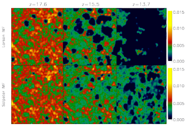
Figure 30: Slice through the simulation boxes. The six panel show the neutral hydrogen number density for the case of a Larson IMF with $M_{c}=5\;M_{\odot}$ (upper panels) and for a Salpeter IMF (lower panels) at redshifts, from left to right, $z=17.6,\;15.5$ and $13.7$. The escape fraction is 20%. The box for the radiative transfer simulation has a comoving length of $L=20h^{-1}$ Mpc. This Figure is taken from Ciardi et al. (2003).

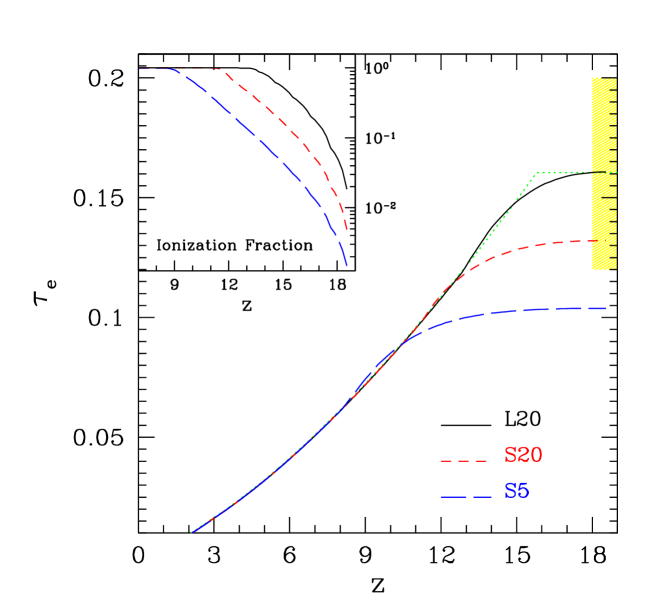
Figure 31: Redshift evolution of the electron optical depth, $\tau_{e}$, for an Salpeter IMF with $f_{esc}=5$% (long-dashed line) and $f_{esc}=20$% (short-dashed line), and for a Larson IMF with $M_{c}=5\;M_{\odot}$ and $f_{esc}=20$%. The dotted line refers to a sudden reionization at $z=16$. The shaded region indicates the optical depth $\tau_{e}=0.16\pm 0.04$ (68% CL) implied by the Kogut et al. (2003) ‘model independent’ analysis. In the inset the redshift evolution of the volume-averaged ionization fraction, $x_{v}$, is shown for the three runs. This Figure is taken from Ciardi et al. (2003).

Abel T., Anninos P., Zhang Y. & Norman M. L., 1997, NewA, 2, 181

Abel T., Bryan G. L., Norman M. L. 2000, ApJ, 540, 39

Balbus S. A., 1995, The Physics of the Interstellar Medium and Intergalactic Medium, ASP Series Vol. 80 (San Francisco: PASP) p. 328

Bajtlik S., Duncan R. C. & Ostiker J. P., 1998, ApJ, 327, 570

Becker R. H. et al., 2001, AJ, 122, 2850

Benson A. J., Lacey C. G., Bauch C. M., Cole S., Frenk C. S., 2002, MNRAS, 333, 156

Benson A. J. & Madau P., 2003, MNRAS, 344, 835

Bianchi S., Cristiani S. & Kim T.-S., 2001, A&A, 376, 1

Boyle B. J., Shanks T., Croom S. M., Smith R. J., Miller L., Loaring N., Heymans C., 2000, MNRAS, 317, 1014

Bromm V., Coppi P. S., Larson R. B. 1999, ApJ, 527, L5

Bromm V., Coppi P. S., Larson R. B. 2002, ApJ, 564, 23

Bromm V., Ferrara A., Coppi P. S., Larson R. B., 2001, MNRAS, 328, 969

Bruzual A. G. & Charlot S., 2003, MNRAS, 344, 1000

Cen R., 2003, ApJ, 591, 12

Ciardi B., Ferrara A. & Abel T., 2000, ApJ, 533, 594

Ciardi B., Ferrara A., Governato F. & Jenkins A., 2000, MNRAS, 314, 611

Ciardi B., Ferrara A., Marri S. & Raimondo G., 2001, MNRAS, 324, 381

Ciardi B., Ferrara A. & White S. M. D., 2003, MNRAS, 344, L7 astro-ph/0302451

Cioffi D., McKee C. F. & Bertschiger E., 1988, ApJ, 334, 252

Cooke A. J., Espey B. & Carswell R. F., 1997, MNRAS, 284, 552

Dawson S., Spinrad H., Stern D., Dey A., van Breugel W., de Vries W., & Reuland M., 2002, ApJ, 570, 92

Dekel A. & Silk J., 1986, ApJ, 303, 39

Dey A., Spinrad H., Stern D., Graham J. R., & Chaffee F. H., 1998, ApJ, 498, 93

Dove J. B., Shull J. M. & Ferrara A., 2000, ApJ, 531, 846

Ellis R., Santos M. R., Kneib J.-P., Kuijken K., 2001, ApJL, 560, 119

Fan X. et al., 2002, AJ, 123, 1247

Ferrara A. & Tolstoy E., 2000, MNRAS, 313, 291

Field G. B., 1995, ApJ, 142, 531

Fryer G. M., 1999, ApJ, 522, 413

Fryer G. M., Woosley S. E. & Weaver T. A., 2001, ApJ, 550, 372

Fujita S. S. et al. 2003, AJ, 125, 13

Furlanetto S. R. & Loeb A., 2003, ApJ, 588, 18

Giallongo E., Cristiani S., D’Odorico S., Fontana A. & Savaglio S., 1996, ApJ, 466, 46

Giallongo E., Fontana A., Cristiani S. & D’Odorico S., 1999, ApJ, 510, 605

Haardt & Madau, 1996, ApJ, 461, 20

Heger A. & Woosley S. E., 2001, ApJ, 567, 532

Hu E. M., Cowie L. L., McMahon R. G., Capak P., Iwamuro F., Kneib J.-P., Maihara T., & Motohara K., 2002, ApJ, 568, L75

Hu E. M., McMahon, R. G., Cowie, L. L., 1999, ApJ, 522, L9

Kim T.-S., Cristiani S. & D’Odorico S., 2002, A&A, 383, 747

Kodaira K. et al. 2003,PASJ, 55, 17

Kogut A. et al., 2003, ApJS, 148, 161

Larson R. B., 1974, MNRAS, 169, 229

Lehnert M. D. & Bremer M., 2003, ApJ, 593, 630

Mac Low M.-M. & Ferrara A., 1999, ApJ, 513, 142

Madau P., Ferrara A. & Rees M., 2001, ApJ, 555, 92

Madau P. & Rees M. J., 2001, ApJ, 551, L27

Marri S. et al. 2003, in preparation

Marri S. & White S. D. M., 2003, MNRAS, 345, 561

McKee C. F. & Draine B. T., 1991, Science, 252, 397

Mori M., Ferrara A. & Madau P., 2002, ApJ, 571, 40

Navarro J. F. & White S. D. M., 1993, MNRAS, 265, 271

Norberg P. et al., 2002, MNRAS, 336, 907

Omukai K., 2001, ApJ, 546, 635

Omukai K. & Inutsuka S. 2002, MNRAS, 332, 59

Omukai K. & Palla F. 2003, ApJ, 589, 677

Osterbrok D. E., 1989, Astrophysics of Gaseous Nebulae and Active Galactic Nuclei, (Mill Valley: University Science Books)

Ostriker J. P. & McKee C. F., 1988, Rev. Mod. Phys., 60, 1

Pearce F. R. et al., 1999, ApJ, 521, 99

Persic M., Salucci P., Stel F., 1996, MNRAS, 281, 27

Ricotti M., Ferrara A. & Miniati F., 1997, ApJ, 485, 254

Rhoads J. E. et al., 2003, AJ, 125, 1006

Scannapieco E., Ferrara A. & Broadhurst T., 2000, ApJL, 536, 11

Scannapieco E., Ferrara A. & Madau P., 2002, ApJ, 574, 590

Scannapieco E., Schneider R. & Ferrara A., 2003, ApJ, 589, 35

Schaerer D., 2002, A&A, 382, 28

Schaye J., Rauch M., Sargent W. L. W. & Kim T.-S., 2002, ApJL, 541, 1

Schneider R., Ferrara A., Natarayan P. & Omukai K., 2002, ApJ, 571, 30

Schneider R., Ferrara A., Salvaterra R., Omukai K. & Bromm V., 2003, Nature, 422, 869

Scott J., Bechtold J., Dobrzycki A. & Kulkarni V. P., 2000, ApJS, 130, 67

Sedov L., 1978, Similitude et Dimensions en Mecanique, (Moscow: Editions de Moscou)

Spizer L., 1978, Physical Processes in the Interstellar Medium, (Whiley: New York)

Silk J., 2003, MNRAS, 343, 249

Steidel C. C., Pettini M. & Adelberger K. L., 2001, ApJ, 546, 665

Tegmark M. et al., 1997, ApJ, 474, 1

Thacker R. J. & Couchman H. P., 2001, ApJ, 555, L17

Thomas P. A., Fabian A. C., Arnaud K. A., Forman W., Jones C., 1986, MNRAS, 222, 655

Tumlinson J., Giroux M. & Shull J. M., 2001, ApJ, 555, 839

Umeda H. & Nomoto K., 2002, ApJ, 565, 385

White S. D. M. & Frenk C. S., 1991, ApJ, 379, 52

Wyithe S. & Loeb A., 2003, ApJ, 588, 69

Wolfire M. G., Hollenbach D., McKee C. F., Tielens A. G. G. M. & Bakes E. L. O., 1995, ApJ, 443, 152