The Maxwell–Boltzmann gas with non-standard self–interactions: a novel approach to galactic dark matter
Abstract
Using relativistic kinetic theory, we study spherically symmetric, static equilibrium configurations of a collisionless Maxwell-Boltzmann gas with non-standard self-interactions, modelled by an effective one–particle force. The resulting set of equilibrium conditions represents a generalization of the classical Tolman-Oppenheimer-Volkov equations. We specify these conditions for two types of Lorentz–like forces: one coupled to the 4-acceleration and the 4–velocity and the other one coupled to the Riemann tensor. We investigate the weak field limits in each case and show that they lead to various Newtonian type configurations that are different from the usual isothermal sphere characterizing the conventional Newtonian Maxwell–Boltzmann gas. These configurations could provide a plausible phenomenological and theoretical description of galactic dark matter halo structures. We show how the self–interaction may act phenomenologically as an effective cosmological constant and discuss possible connections with Modified Newtonian Dynamics (MOND).
pacs:
04.20.Cv, 47.75.+f, 95.35.+d, 98.35.GiI Introduction
There is a broad consensus that both on cosmological and on galactic scales substantial amounts of dark matter are needed to explain current observations. Recent data from type Ia supernovae, the large-scale-structure analysis, and the anisotropies of the cosmic microwave background (CMB) suggest that the dynamics of the present Universe is determined by a mixture of roughly 70 dark energy and roughly 30% (cold) dark matter (CDM). To understand the physical nature of these main ingredients of the cosmic substratum is one of the basic challenges in current cosmology. Numerous models have been worked out over the past few years, the most popular one still being the CDM model which also plays the role of a reference setting for competing scenarios, such as the different quintessence models, which are based on the dynamics of a scalar field with a suitable potential Qmatter ; Qmatter2 . In some models interacting quintessence played a crucial role intQ1 ; intQ2 . Furthermore, the cosmic medium has also been modelled as a gas with non-standard interactions given in terms of an effective one-particle force gasQ1 ; gasQ2 ; gasQ3 ; gasQ4 .
Regarding dark matter (DM), the CDM paradigm of collisionless (yet undetected) supersymmetric particles is successful at the cosmological scale Ellis ; Fornengo , though some of its predictions at the galactic scale (“cuspy” density profiles and excess substructure) have been at odds with observations cdm_problems_1 ; cdm_problems_2 . It is natural then to look for DM models with some type of phenomenological self–interaction scdm , but because of the unknown nature of DM in galactic halos, the type of self-interaction is also an open question. Hence, other models (“warm” DM) consider lighter more thermal particles wdm and even non–thermal sources, such as coherent scalar fields have been contemplated sfdm1 ; sfdm2 ; sfdm3 ; sfdm4 .
Since DM in galactic halos constitutes about of the mass of galactic systems, while the latter have Newtonian characteristic velocities, the dynamics of these systems is usually examined within a Newtonian framework in which, as a first approximation, visible matter can be considered as test particles in the gravitational field of the DM halo. The standard models are either idealized configurations of collisionless matter obtained from Newtonian kinetic theory BT , or models based on n–body numerical simulations nbody_1 ; nbody_2 ; nbody_3 that yield “universal” density or rotation velocity profiles urc ; DMprofs1 ; DMprofs2 ; DMprofs3 . While the usual Newtonian approach may well be adequate on galactic scales, only a general relativistic setting can provide limits for the validity of the Newtonian approximation. In a general relativistic treatment in which DM provides the bulk of spacetime curvature, the motion of baryonic matter can be treated as test particle motion in the geometry generated by the DM (“rotation velocities” become then velocities of circular geodesic orbits HGDM ; Lake ). However, a relativistic approach will not only yield corrections to the Newtonian case, but it also provides a framework which admits theoretical generalizations, e.g. the introduction of non-standard interactions in a systematic and self–consistent way. It is this property, which will be relevant for the present paper. Given the unknown nature of the halo matter, it seems to be of interest to consider various types of non–standard interactions within this matter and to explore the consequences of such an assumption. Matter with self-interaction may have a Newtonian type limit which differs from the standard Newtonian limit for non-interacting dark matter. This property is demonstrated here for two choices of a self-interaction. On this basis it becomes possible to discuss modifications of standard astrophysical configurations where the focus of the present paper is on isothermal spheres.
Gas models allow interactions to be described by effective one-particle forces. To obtain candidates for potentially interesting self-interactions we follow a strategy similar to the one which was previously used in a cosmological context gasQ1 ; gasQ2 ; gasQ3 . These investigations demonstrated that the admissible structure of the relevant forces is severely restricted by the symmetries of the problem (which are the symmetries of the cosmological principle in gasQ1 ; gasQ2 ; gasQ3 ). In the present paper we apply this formalism for the first time to a galactic scale in which astrophysical systems (DM halos) are necessarily inhomogeneous, hence we consider a spherically symmetric and static geometry. The latter is then combined with the equilibrium conditions of a Maxwell–Boltzmann (MB) gas in the presence of a self-interacting force field. On the fluid level this force generates effective pressures, representing additional degrees of freedom that extend the classical Tolman–Oppenheimer–Volkov (TOV) analysis. We demonstrate that the resulting configurations provide modifications of the usual isothermal sphere (the Newtonian limit of a “standard” MB gas), which have the potential to provide adequate phenomenological and theoretical descriptions of galactic DM. As a particular feature, the interaction, introduced here in a general relativistic framework, takes the form of an additional Newtonian type force in the corresponding limit. This indicates possible relations to Modified Newtonian Dynamics (MOND) MOND although, different from the latter, the interaction here is an interaction within the DM.
The present paper also provides a generalization of previous well established work on relativistic kinetic theory of collisionless matter applied to globular clusters prevRKT (though our focus here is on DM halos).
The paper is organized as follows: sections II and III present the general formalism of relativistic kinetic theory with self–interactions modelled as a one particle force. In sections IV and V we obtain the full general relativistic equilibrium equations for a static, spherically symmetric spacetime. We specialize in section VI to a Lorentz–like force, linear in the particle momenta and without anisotropic stresses. In section VII we consider two possible cases of covariant couplings of this Lorentz–like force: firstly, to the 4–acceleration and the 4–velocity and secondly, to the Riemann tensor. Section VIII investigates two types of Newtonian type limits: a “standard” Newtonian limit that yields modified isothermal configurations and a Newtonian type limit in which the generalized force acts as an effective cosmological constant. Two numerical examples of configurations constructed with each type of Newtonian limit are discussed in section IX, while section X provides a summary and conclusion.
II Kinetic Theory
We assume that the particles of a collisionless relativistic gas move under the influence of a 4-force field . The equations of motion of the gas particles are kinetic
| (1) |
where is a parameter along the particle worldlines. Since the particle 4-momenta are normalized according to with constant mass , the force must satisfy . The corresponding equation for the invariant one-particle distribution function may be written as
| (2) |
We shall restrict ourselves to the class of forces which admit solutions of (2) that are of the type of the Jüttner distribution function
| (3) |
where and is a timelike four vector. The particle number flow 4-vector, , and the equilibrium energy-momentum tensor, , are then defined in a standard way (see, e.g., kinetic ) as
| (4a) | |||||
| (4b) | |||||
Here, the integrals are over the mass shell const in momentum space. For the balance equations we find
| (5) | |||||
| (6) | |||||
where the semicolon denotes the covariant derivative.
III Symmetry considerations
The quantities and may be split with respect to the unique 4-velocity as
| (7) |
where is the spatial projection tensor . The scalars can be, respectively, identified with the particle number and matter–energy densities and the equilibrium pressure. Inserting (3) into (2) yields the constraint
| (8) |
In order to make further progress, we have to introduce assumptions about . Guided by the analogy to the Lorentz force, we shall consider a force that is linear in the particle momentum, i.e.
| (9) |
where is a function of the spacetime coordinates but does not depend on the particle momentum . Since the force has to satisfy , it follows that, analogously to the Lorentz-force, is valid. As a consequence we have and the condition (8) decomposes into
| (10) |
As opposed to the case of the Lorentz force, the quantity is not specified here. We only require that it should be compatible with the integrability condition which holds for spherically symmetric static spacetimes to be discussed below. The second relation in (10) implies that is a timelike Killing vector, which gives rise to the relations
| (11) |
where is the equilibrium temperature and
| (12) |
where . Because of the antisymmetry of the first of the relations (10) splits into
| (13) |
Using the force (9) in the energy-momentum balance (6), we obtain
| (14) |
The projection of (6) in direction of is satisfied identically, since and the right hand side of the resulting equation also vanishes.
It is interesting to consider the Gibbs-Duhem relation
| (15) |
where is the chemical potential. With the identification (23) this yields
| (16) |
which is completely general and quite independent of the action of a force. Obviously, the consistency between the last relation and the momentum balance (14) is guaranteed through (12).
The energy-momentum tensor is not conserved and therefore it is not a suitable quantity in Einstein’s field equations. Following earlier considerations in a cosmological context gasQ1 ; gasQ2 ; gasQ3 ), we try to map the “source” terms in the balances for on imperfect fluid degrees of freedom of a conserved energy-momentum tensor of the form
| (17a) | |||||
| (17b) | |||||
| (17c) | |||||
where we can identify as the scalar off-equilibrium pressure, as the traceless anisotropic stress tensor and as the energy flux vector. Since we must have , then
| (18) |
which in the present case without an energy flux reduces to
| (19) | |||||
All these relations do not depend on a specific choice of the antisymmetric quantity in (9). Consequently, on the fluid level the additional interaction manifests itself through the appearance of the additional pressure contributions and .
In the following we are interested in the limit in which the “equilibrium” state variables introduced in (7) satisfy the equation of state of a non-relativistic Maxwell-Boltzmann (MB) gas kinetic with rest mass–energy density ,
| (20) |
with
| (21) |
where
| (22) |
is the “relativistic coldness” parameter. Therefore, is the fugacity scalar that is related to the chemical potential by
| (23) |
IV Spherically symmetric and static spacetime
We now apply the formalism outlined so far to a spherically symmetric and static spacetime, whose metric can be given as
| (24) | |||||
where and have, respectively, units of velocity squared and mass. Our strategy is to combine the corresponding field equations with the equilibrium conditions of the previous section. Then the 4–velocity and the 4–acceleration (in velocity and acceleration units) take their customary forms
| (25) |
Other relevant quantities are
| (26a) | |||||
| (26b) | |||||
where a prime denotes derivative with respect to . Equation (12) implies the well known Tolman law , which remains valid here for any choice of in (9).
Particle motion in a spherically symmetric field is characterized by conservation of the of the angular momentum . But with the particles do not follow geodesics and so is not a constant of motion. In the present case the force may be written as , hence the two nonzero components of are
| (27a) | |||||
where
| (28) |
and we have eliminated from and used , as well as conservation of angular momentum. The equilibrium condition (13) for becomes
| (29) |
Notice that and have, respectively, units of acceleration and force.
V Field equations
For the metric (24), we have and the most general form of the spacelike traceless tensor is given by , where is an arbitrary function. Thus, the momentum–energy tensor is
leading for (24) and (LABEL:Tab_ss) to the field equations (or “equilibrium” TOV type equations)
| (31) | |||||
| (32) |
where, from (20) and (21), we know that and are functions of and . This has to be complemented by (29) and by
| (33) |
| (34) |
In the absence of the additional interaction, i.e. for , we recover the standard TOV equations while Eq. (34) reduces to .
Assuming to be known, equations (31)–(34), complemented by (20) and (21), constitute a system of five differential equations for six unknowns: . Hence, an extra constraint is needed to render this system determinate. One way of achieving this determinacy is to provide a specific relation between and . The simplest cases are either one of
| (35a) | |||||
| (35b) | |||||
Another possible approach follows by defining “radial” and “tangential” pressures as
| (36) |
leading to a system like (31)–(34), with (32) and (34) replaced by
| (37) | |||||
| (38) |
where
| (39) |
is the “anisotropy factor”. If the latter is selected (say, from empirical considerations) we have also a determined system.
VI Linear isotropic case
We consider now the case in which is linear in the momentum , with purely isotropic stresses characterized by (or ). The system (31)–(34) reduces to
| (40a) | |||||
| (40b) | |||||
| (40c) | |||||
| (40d) | |||||
where we used (20) and (21) to eliminate and in terms of and , with and given by
| (41a) | |||||
| (41b) | |||||
where the subscript c will denote henceforth evaluation at the symmetry center . It is convenient for self gravitating gas sources to eliminate in terms of the velocity dispersion of gas particles BT
| (42) |
and to express in terms of the dimensionless variable
| (43) |
which reduces to the “normalized” Newtonian potential in the Newtonian limit. Equations (41a) and (41b) then become
| (44b) | |||||
where
| (45) |
We introduce the dimensionless variables
| (46a) | |||||
| (46b) | |||||
| (46c) | |||||
| (46d) | |||||
where we have used:
With the definition (42) the parameter in Eq. (45) represents a dimensionless velocity dispersion of the particles. A corresponding quantity, the parameter defined in Eq. (21), arises due to the existence of the additional pressure . Both these parameters will be relevant for the Newtonian type limits discussed below. In terms of the parameters defined in (46) the system (40a)–(40d) becomes
| (47a) | |||||
| (47b) | |||||
| (47c) | |||||
| (47d) | |||||
where we have eliminated from (44b), while follows from (LABEL:eqrho3). We emphasize again, that this set of equation is valid for any force of the type (9). Although for an explicit evaluation we might propose any functional form , it is more convenient to provide a covariant form for .
VII Specific forces
While the assumed structure (9) of the force shares some features of the Lorentz force, its explicit functional form has been left open. The accelerations are only restricted by the symmetry requirement . Since we expect this force to model an effective interaction, it may self-consistently depend on the macroscopic fluid quantities in addition to its (fixed, linear) dependence on the microscopic particle momentum.
VII.1 First case
A simple choice for an antisymetric tensor for a spherically symmetric fluid spacetime is
| (48) |
which, for the metric (24) and using the variables (46), yields
| (49) | |||||
while the components of are
| (50a) | |||||
Thus, the dimensionless quantity is the free parameter (not necessarily constant) which determines the functional form of the force strength.
VII.2 Second case
An interaction mediated by the curvature provides another choice of an antisymmetric tensor :
| (52) |
where is a characteristic length scale and are the components of the curvature tensor, hence the corresponding interaction is non–minimal. Now, forces which are proportional to the curvature tensor are usually not admitted in General Relativity since they violate the equivalence principle. Here, it is the self-consistent mapping of the corresponding source terms on imperfect fluid degrees of freedom of a conserved energy momentum tensor according to (17a) - (17c), which allows us to consider this force as an internal interaction within Einstein’s theory.
VIII Newtonian type limits
Since our approach implies a non-standard degree of freedom, we have to define what we mean by a Newtonian type limit. The free parameter defined in (45) is associated with the characteristic velocities of a spherically symmetric MB gas. The second free parameter in (46) is new and provides the velocity dispersion associated with the additional pressure . It quantifies the impact of the non-standard interaction on our equilibrium configuration. We expect this impact to be a small correction to the standard case (the case without additional interaction), hence . Since the dimensionless quantities and are not necessarily “small”, it is reasonable to consider a weak field limit based on the conditions
| (58) |
irrespective of how and are related. The metric functions in (24) become up to first order in
while applying (58) to (LABEL:eqrho3) we obtain
| (60) |
Newtonian type limits imply Newtonian particle velocities and . Under the conditions (58) we also have and , hence the components of given by (27) become
| (61) |
so that . Conditions (58) imply a weak field limit which can be identified with various types of “nearly Newtonian” conditions that are obtained by comparing and and by expanding all incumbent variables with respect to either one (or both) of these dimensionless ratios.
VIII.1 The “standard” Newtonian limit
In the general relativistic treatment of the “standard” MB gas (without self–interaction mediated by , so that: ) the Newtonian limit follows by expanding all relevant quantities up to first order in . This leads to the “isothermal sphere” with relativistic corrections of order . An equivalent Newtonian limit can be defined for the case if together with (58) we have
| (62) |
so that and the relativistic correction introduced by is of the same order but smaller than the thermal one, corresponding to the equilibrium hydrostatic pressure . By expanding up to we get modifications of the isothermal sphere characterized by the post–newtonian equilibrium equations
| (63a) | |||||
| (63b) | |||||
| (63c) | |||||
| (63d) | |||||
with given by (60).
VIII.1.1 First case
If we assume (48), we have in the weak field limit
| (64) |
and so the components of the force are
| (65) |
where we have eliminated from (40b). The Newtonian structure of the force in this limit is obvious. The equilibrium equations are then (63), with (63c) and (63d) replaced by
| (66a) | |||||
| (66b) | |||||
The fact that the additional interaction, introduced in a general relativistic setting, reduces to an additional Newtonian type force (65) in the appropriate limit reminds of corresponding features of Modified Newtonian Dynamics (MOND) MOND . While the latter, however, was introduced as an alternative to DM, the force describes a self-interaction within the DM in our case. Nevertheless, our result does not seem to exclude an approach in which the DM is replaced by baryonic matter with a modified Newtonian limit of a general relativistic description, where the modification is a consequence of a non-geodesic motion of the (baryonic) particles of the medium. We plan to follow this line in future work.
VIII.1.2 Second case
VIII.2 Newtonian limit with a repulsive force
If instead of (62) we choose (58) together with
| (70) |
then, instead of (63), the equilibrium equations in the Newtonian limit are
| (71a) | |||||
| (71b) | |||||
| (71c) | |||||
| (71d) | |||||
with given by (60). If , then equation (71d) implies , hence
| (72) |
But if (a more likely outcome), then the form of cannot be guessed before a numerical integration. Still, the term in (71b) behaves as a repulsive force similar to a positive “cosmological constant” that can be associated with the matter–energy density SussHdez
| (73) |
The equilibrium equations in each case follow by inserting in (71) the appropriate form of and taking . For the first case we have
| (74) |
with
| (75) |
For the second case we have
| (76) |
with
| (77) |
IX Numerical examples
We examine separately two configurations, one for each form of the
generalized forces (48) and (52). These examples
aim at illustrating how the formalism we have introduced works in
practice. Although these examples are not meant to describe
“realistic” models of equilibrium systems, they show how
generalized forces in collisionless gases might influence known
velocity and density profiles and hence are of
interest in astrophysical applications.
IX.1 A modified isothermal sphere
Let us consider a generalized force complying with (48), with the dimensionless parameter given by
| (78) |
In the “standard” Newtonian limit (58) and (62) with , we obtain hydrostatic configurations that resemble the isothermal sphere (case without force). Assuming the parameters characteristic of a galactic dark matter halo similar to that of the Milky Way ranges :
| (79) |
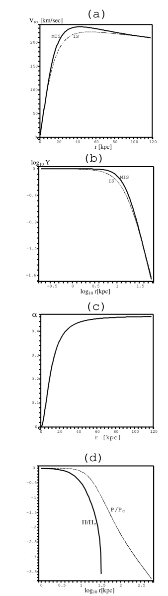
we integrate the equilibrium equations (63a), (63b), (66a) and (66b) and show the results in figure 1, where solid curves (marked as “MIS”) denote the modified isothermal sphere in comparison with the curves corresponding to the isothermal sphere (dotted curves marked as “IS”). Figure 1(a) displays the rotation velocity profile obtained from (37), (47b) and (63b)
| (80) |
The profile is qualitatively analogous to the isothermal one, but reveals slight differences from the latter already in the region occupied by visible matter (up to a radius of kpc): it is steeper near the center and reaches a higher maximal velocity. Instead of the “flat” isothermal profile, the present case shows a slight decay in . Figure 1(b) shows the density profile, , which reveals a wider “flat core” region with the same asymptotic decay of the isothermal sphere. Figure 1(c) displays the function , while figure 1(d) compares the curve for the pressure associated with the generalized force, with that for the hydrostatic pressure . While , as in the isothermal case, decays exponentially.
It is worthwhile mentioning that similar models of modified isothermal spheres can be obtained with the curvature coupled force (52), though we will use this type of force to model an effective cosmological constant.
IX.2 Cosmological constant from curvature coupling
Assuming a curvature mediated force (52), we examine now the case of a weak field limit that resembles an isothermal sphere in equilibrium with a cosmological constant (i.e. a cosmological field with matter–energy density SussHdez ). This suggests a generalized force of cosmic origin, characterized by very large length scales. In fact, from (55) with km/(sec Mpc),
| (81) |
where we have used and (79), it follows that corresponds to a characteristic length scale of Mpc, roughly an order of magnitude larger than the size of the largest galactic clusters in virialized equilibrium (it is roughly the size of a supercluster padma ). Following (73), the ratio of central hydrostatic pressure to the pressure of the –field is
| (82) |
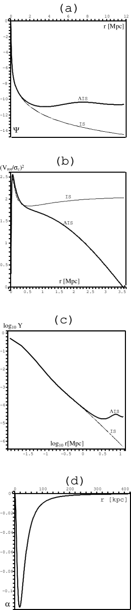
where we have used (79), as well as and . Hence, in order to have a curvature mediated force acting as a cosmological constant, it is reasonable to assume , together with conditions (70) with . Notice that the rotation velocity profile is no longer given by (80), but by
| (83) |
We integrate the equilibrium equations (71) for the
values (79), with given by (76),
displaying the results in Fig. 2. Figures 2(a)–2(c) show how the
normalized potential, , the velocity squared and density
profiles, and , are practically
indistinguishable from the curves of these same variables in the
case of an isothermal sphere coupled to a cosmological constant
(see SussHdez for a comparison and a detailed discussion of
this system). As figure 2(a) shows, the function
oscillates, indicating “turning points” where that
separate regions with different signs of . The density
profile in figure 2(c) does not decay asymptotically as ,
as the isothermal profile, but oscillates around the density value
of the “background” –field. At the first turning point
of the squared velocity (figure 2(b)) vanishes
and becomes negative (hence circular geodesic orbits cannot exist
for larger ). Notice that this first turning point occurs at
Mpc, about an order of magnitude larger than the
physical radius of an isothermal halo similar to the Milky Way. As
discussed in SussHdez , this fact allows one to ignore the
effects of a cosmological constant in the equilibrium of galactic
DM halos. A phenomenological analogue of a cosmological constant
can also be achieved by applying conditions (70) to
a force given by the coupling (48), though we have
preferred to illustrate this analogue with the case (52)
because it offers a more natural association with a cosmic force
acting on very large length scales.
X Discussion and conclusion
We have derived the hydrostatic equilibrium conditions for a gas with a specific class of self-interactions in a spherically symmetric spacetime. This self-interaction is described by a Lorentz–like force (9) that is linear in the particle momentum and characterized by a Maxwell–like antisymmetric tensor . Within this framework, we have considered two possible covariant forms for this force that are adequate for the static and spherically symmetric spacetime geometry: the one given in equation (48) where this tensor is proportional to , the other given in equation (52), coupling it to the Riemann tensor. The equilibrium equations in each case were presented in terms of dimensionless variables, which allowed us to obtain the Newtonian type limit in a natural way by expanding with respect to the dimensionless parameters and , which characterize the dispersion velocities associated with the hydrostatic ideal gas pressure, , and the pressure , respectively, the latter being the result of the self–interaction on the hydrodynamic level. We have provided two numerical examples of Newtonian type weak field configurations, a modified isothermal sphere and an example of how the curvature coupled force can act phenomenologically as an effective cosmological constant.
While we do not claim the examples introduced in section IX and depicted by figures 1 and 2 to describe “realistic” configurations, we believe that these simplest possible cases nevertheless do illustrate how configurations of astrophysical interest might arise from the presented formalism. In fact, these models, especially that of the modified isothermal sphere shown in figure 1, do convey interesting information worth discussing. For example, numerical simulations nbody_1 ; nbody_2 ; nbody_3 ; urc ; DMprofs1 ; DMprofs2 ; DMprofs3 yield halo configurations characterized by empiric density and velocity profiles that differ from the isothermal profiles, at least in the inner halo region containing a disk of baryonic matter (which can be considered as “tracers” of the halo gravitational field). The non–isothermal velocity profile associated with the Navarro–Frenk–White (NFW) and analogous simulations nbody_1 ; nbody_2 ; nbody_3 , as well as other velocity profiles urc ; DMprofs1 ; DMprofs2 ; DMprofs3 , are qualitatively similar to the velocity profile shown by the solid curve in Fig. 1(a), corresponding to an MB gas with a generalized force of the type (48). Surprisingly, the empiric density profiles of these simulations show a “density peak” towards the halo center which does not match the density profile of Fig. 1(c) that shows a “flat density core”. Numerical simulations also yield an asymptotic decay , that is different from the isothermal decay of figure 1(c) (though it is difficult to verify the asymptotic DM density decay by means of observations). However, observations in low surface brightness (LSB) galaxies vera ; LSB (supposedly dominated by DM) do not reveal the “density peak” predicted by numerical simulations, but an isothermal “flat core” (this is still a hotly controversial issue). Hence, the simple toy model we have proposed in section IX shows a rotation velocity profile compatible with numerical simulations, but without the controversial “density peak”. It is then quite possible that more elaborated models of a MB gas with self–interaction could provide a reasonable phenomenological fit to observations, especially if we consider the case with anisotropic stresses since more realistic galactic halos are very unlikely to correspond to isotropic configurations. Further research in this direction is currently being undertaken.
It is expedient to point out that the interactions studied in this paper seem to share features with MOND MOND . This could provide the theoretical basis for an approach in which the DM is replaced by baryonic matter with a modified Newtonian limit of a general relativistic description. In such a setting modifications of Newton’s law would be the result of a non-geodesic motion of the (baryonic) particles of the medium.
Finally, regarding the
phenomenological modelling of a cosmological constant by means of
the curvature coupled force (52), we have shown that this
self–interaction can reproduce similar effects as those of
previous studies of a cosmological constant (a cosmic
field) in hydrostatic equilibrium with a MB gas (see
SussHdez ). On the other hand, the gas dynamics with
self–interactions of the type that we have presented in this
paper has been successfully applied to dark energy models at the
cosmological scale gasQ1 ; gasQ2 ; gasQ3 ; gasQ4 . Thus, the study
of the interplay and correspondence between galactic scale models,
as those derived here, and those describing the cosmic dynamics
dominated by dark energy provides an interesting and relevant
avenue for further research.
Acknowledgements.
This work was supported by the Deutsche Forschungsgemeinschaft, CONACYT (number E130.792), and by Russian funds RFBR (grant N 04-05-64895) and HW (grant N 1789.2003.02).References
- (1) N. Bahcall, J.P. Ostriker, S. Perlmutter, and P.J. Steinhardt, Science, 284, 1481, (1999).
- (2) J.A.S. Lima, Braz. J. Phys., 34, 194, (2004). e-Print Archive: astro-ph/0402109.
- (3) W. Zimdahl, D. Pavón and L.P. Chimento, Phys. Lett. B, 521, 133, (2001).
- (4) L.P. Chimento, A.S. Jakubi, D. Pavón, and W. Zimdahl, Phys.Rev. D 67, 083513, (2003).
- (5) W. Zimdahl, D.J. Schwarz, A.B. Balakin, and D. Pavón, Phys.Rev. D 64, 063501, (2003).
- (6) W. Zimdahl and A.B. Balakin, Phys.Rev. D 63, 023507, (2001).
- (7) W. Zimdahl, A.B. Balakin, D.J. Schwarz, and D. Pavón, Grav.Cosmol. 8, 158, (2002).
- (8) A.B. Balakin, D. Pavón, D.J. Schwarz, and W. Zimdahl, New J.Phys. 5, 085, (2003).
- (9) J. Ellis, astro-ph/0204059.
- (10) N. Fornengo, Proceedings of Nucl.Phys. Poc. Suppl. 124, 170 (2003).
- (11) B. Moore, Nature (London), 370, 629, (1994).
- (12) R. Flores and J. P. Primack, ApJ, 427, L1, (1994).
- (13) D.N. Spergel and P.J. Steinhardt, Phys Rev Lett., 84, 3760, (2000); A. Burkert, APJ Lett., 534, 143, (2000); C. Firmani, E. D’Onghia, V. Avila-Reese, G. Chincarini, and X. Hernandez, Mon. Not. R. Astron. Soc., 315, 29, (2000).
- (14) S. Colombi, S. Dodelson and L. Widrow, ApJ, 458, 1, (1996); R. Schaeffer and J. Silk, ApJ, 332, 1, (1998); C.J. Hogan, astro-ph/9912549; S. Hannestad and R. Scherrer, Phys. Rev. D, 62, 043522, (2000).
- (15) Tonatiuh Matos and F. Siddhartha Guzmán. Class. Quant. Grav., 17, (2000), L9-L16. See also: Tonatiuh Matos and Luis A. Ureña. Phys Rev. D63, (2001), 063506.
- (16) Miguel Alcubierre, Ricardo Becerril, F. Siddhartha Guzmán, Tonatiuh Matos, Darío Núñez, and L. Arturo Ureña-López. Class. Quant. Grav. , 20, 2883, (2003).
- (17) A. Arbey, J. Lesgourgues and P. Salati, Phys. Rev. D 64, 123528 (2001). See also Phys. Rev. D 65, 083514 (2002). See also: A. Arbey, J. Lesgourgues and P. Salati, Phys. Rev. D 68, 023511 (2003).
- (18) U. Nucamendi, M. Salgado and D. Sudarsky, Phys. Rev. Lett., 84, 3037, (2000).
- (19) J. Binney and S. Tremaine, Galactic Dynamics, (Princeton University, Princeton, NJ, 1987).
- (20) J.F. Navarro, C.S. Frenk and S.D.M. White, ApJ, 462, 563, (1996); see also: J.F. Navarro, C.S. Frenk and S.D.M. White, ApJ, 490, 493, (1997).
- (21) B. Moore, T. Quinn, F. Governato, J. Stadel, and G. Lake, Mon. Not. R. Astron. Soc., 310, 1147, (1999).
- (22) S. Ghigna, B. Moore, F. Governato, G. Lake, T. Quinn, and J. Stadel, astro-ph/9910166.
- (23) E. Battaner and E. Florido, The rotation curve of spiral galaxies and its cosmological implications, Fund. Cosmic Phys. 21, 1 -154, (2000). astro-ph/0010475.
- (24) A. Burkert and J. Silk, Proceedings of the second international conference on “Dark matter in astro and particle physics”, ed. H.V. Klapdor-Kleingrothaus (1999). e-Print astro-ph/9904159.
- (25) P. Salucci and A. Burkert, ApJ Lett, 537, L9, (2001). e-Print astro-ph/0004397.
- (26) L.M. Widrow, Semi–analytic models for dark matter halos. e-Print astro-ph/0003302.
- (27) L.G. Cabral–Rosetti, T. Matos, D. Nunez, and R.A. Sussman, Class. Quant. Grav., 19, (2002), 3603–3615.
- (28) K. Lake, Phys. Rev. Lett., 92, (2004), 051101, gr-qc/0302067.
- (29) M. Milgrom, ApJ 270, 365; 270, 384 (1983); R.H. Sanders and S.S. McGaugh, Ann.Rev.Astron.Astrophys. 40, 263 (2002), arXiv:astro-ph/0204521.
- (30) E.D, Fackerell, Ap.J., 153, 643, (1968). See also: J.R. Ipser, Ap.J., 156, 509, (1969) and J.R. Ray, Ap.J., 257, 578, (1982).
- (31) Non-equilibrium Relativistic Kinetic Theory, J.M. Stewart, Springer, New York, 1971; J. Ehlers in General Relativity and Cosmology, ed. by B.K. Sachs, Academic Press, New York, 1971; W. Israel and J.M. Stewart, Ann.Phys., 118, (1979), 341. Relativistic Kinetic Theory, S.R. de Groot, W.A. van Leeuwen and Ch.G. van Weert, North Holland Publishing Co., 1980.
- (32) C. Firmani, E. D’Onghia, V. Avila-Reese, G. Chincarini, and X. Hernandez, Mon. Not. R. Astron. Soc., 315, 29, (2000). J.J. Dalcanton and C.J. Hogan, ApJ, 561, 35, (2001). P.R. Shapiro and I.T. Iliev, ApJ, 565, L1, (2002). W.J.G. de Blok, A. Bosma and S.S. McGaugh, Mon. Not. R. Astron. Soc., 340, pp 657, (2003).
- (33) R. A. Sussman and X. Hernández, Mon. Not. R. Astron. Soc., 345, 871, (2003).
- (34) T. Padmanabhan, Structure formation in the universe, Cambridge University Press, 1995.
- (35) W.J.G. de Blok, S.S MacGaugh, A. Bosma, and V.C. Rubin, ApJ 552, L23 (2001). S.S. MacGaugh, V.C. Rubin, and W.J.G. de Blok, ApJ 122, 2381 (2201). W.J.G. de Blok, S.S MacGaugh, and V.C. Rubin, , ApJ 122, 2396 (2001). W. J. G de Blok. ArXiv:astro-ph/0311117. J. D. Simon, A. D. Bolatto, A. Leroy, and L. Blitz, arXiv:astro-ph/0310193. E. D’Onghia and G. Lake. arXiv:astro-ph/0309735.
- (36) J.J. Binney and N.W. Evans, Mon. Not. R. Astron. Soc. 327 L27 (2001). Blais-Ouellette, C. Carignan, and P. Amram, arXiv:astro-ph/0203146. C.M. Trott and R.L. Wesbster, Mon. Not. R. Astron. Soc., 334, 621, (2002), arXiv:astro-ph/0203196. P. Salucci, F. Walter, and A. Borriello, arXiv:astro-ph/0206304.