THE ANGULAR MOMENTUM DISTRIBUTION OF GAS AND DARK MATTER IN GALACTIC HALOS

Abstract

We report results of a series of non radiative N-body/SPH simulations in a $\Lambda CDM$ cosmology, designed to study the growth of angular momentum in galaxy systems. A sample of 41 halos of differing mass and environment were selected from a cosmological N-body simulation of size $32.5h^{-1}$Mpc, and re-simulated at higher resolution with the tree-SPH code GADGET.

We find that the spin of the baryonic component correlates well with the spin of the dark matter, but there is a misalignment of typically $20^{\circ}$ between these two components. The spin of the baryonic component is also on average larger than that of the dark matter component and we find this effect to be more pronounced at lower redshifts. A significant fraction $f$ of gas has negative angular momentum and this fraction is found to increase with redshift. This trend can be explained as a result of increasing thermalization of the virializing gas with decreasing redshift. We describe a toy model in which the tangential velocities of particles are smeared by Gaussian random motions. This model is successful in explaining some of the global angular momentum properties, in particular the anti-correlation of $f$ with the spin parameter $\lambda$ , and the shape of the angular momentum distributions.

We investigate in detail the angular momentum distributions (AMDs) of the gas and the dark matter components of the halo. We compare and contrast various techniques to determine the AMDs. We show that broadening of velocity dispersions is unsuitable for making comparisons between gas and dark matter AMDs because the shape of the broadened AMDs is predominantly determined by the dispersion and is insensitive to the underlying non broadened AMD. In order to bring both gas and dark matter to the same footing, we smooth the angular momentum of the particles over a fixed number of neighbors. The AMDs obtained by this method have a smooth and extended truncation as compared to earlier methods. We find that an analytical function in which the differential distribution of specific angular momentum $j$ is given by $P(j)=\frac{1}{j_{d}^{\alpha}\Gamma(\alpha)}(j)^{\alpha-1}e^{-j/j_{d}}$, where $j_{d}=j_{tot}/\alpha$, can be used to describe a wide variety of profiles, with just one parameter $\alpha$. The distribution of the shape parameter $\alpha$ for both gas and dark matter follows roughly a log-normal distribution. The mean and standard deviation of $log(\alpha)$ for gas is $-0.04$ and $0.11$ respectively. About $90-95\%$ of halos have $\alpha<1.3$, while exponential disks in NFW halos would require $1.3<\alpha<1.6$. This implies that a typical halo in simulations has an excess of low angular momentum material as compared to that of observed exponential disks, a result which is consistent with the findings of earlier works. $\alpha$ for gas is correlated with that for dark matter (DM) but they have a significant scatter $<\alpha_{Gas}/\alpha_{DM}>=1.09\pm 0.2$. $\alpha_{Gas}$ is also biased towards slightly higher values compared to $\alpha_{DM}$. The angular momentum in halos is also found to have a significant spatial asymmetry with the asymmetry being more pronounced for dark matter.

1. Introduction

Disk galaxies are rotationally supported systems and their structural properties are intimately linked to their angular momentum distribution. The standard picture of formation of disk galaxies is that the density perturbations grow due to gravitational instability and end up forming virialized systems of dark matter and gas. The gas cools and collapses towards the center (1978MNRAS.183..341W). The gas has angular momentum which it acquires due to tidal interactions. This can be quantified in terms of a dimensionless spin parameter $\lambda=J|E|^{1/2}/(GM^{5/2})$ (1969ApJ...155..393P) which has a value of about $0.05$ (1979MNRAS.186..133E; 1987ApJ...319..575B; 1995MNRAS...272..570B). The angular momentum of the gas is conserved during the collapse resulting in the formation of a centrifugally supported disk, whose size is consistent with that of observed disk galaxies (1980MNRAS.193..189F).

Based on the initial density profiles ($\rho=\rho(r)$) and angular momentum distributions ($m=m(j)$) or ($M_{<j}=M_{<j}(j)$) the final surface density of disks can be determined. 1997ApJ...482..659D derived the surface density of the disks assuming the halos to be uniform spheres in solid body rotation. From numerical simulations it is now known that density profiles of dark matter in halos follow a universal profile as described by 1996ApJ...462..563N; 1997ApJ...490..493N. Using these realistic profiles and assuming the final surface density of disks to be exponential 1998MNRAS.295..319M investigated various properties of disks like rotation curves, disk scale lengths and so on. They also addressed the issue of stability of disks. However, angular momentum distributions are required to more realistically model the surface density of disk galaxies. 2001ApJ...555..240B have reported that in CDM simulations, the DM halos obey a universal angular momentum distribution of the form

$$\frac{M(<j)}{M_{v}}=\frac{\mu j}{j_{0}+j}$$ (1)

where $j$ is the specific angular momentum and $M(<j)$ is mass with specific angular momentum less than $j$. The shape parameter $\mu$ has a log-normal distribution and the $90\%$ range is given by $1.05<\mu<2.0$. Assuming that the angular momentum profile of gas is identical to that of dark matter, B2001 calculated the surface density profiles of the resulting disks, and found that (for the range of $\mu$ given above) the resulting disks are too centrally concentrated compared to exponential profiles. In addition, detailed hydrodynamical simulations of gas collapse in hierarchical structure formation scenario exhibit the so-called “angular momentum catastrophe”: the gas component looses its angular momentum due to dynamical friction and ends up forming disks that are far too concentrated (1991ApJ...380..320N; 1994MNRAS.267..401N; 1997ApJ...478...13N; 1999ApJ...513..555S).

Recently 2002ApJ...576...21V (henceforth vB2002) has tested the assumption, that the AMDs of gas and DM are similar, by directly measuring the AMDs of gas in proto galaxies from hydrodynamical simulations at $z=3$. They find the spin parameter distribution of gas and dark matter to be identical in spite of the angular momentum vectors of gas and dark matter being misaligned by $\sim 35^{\circ}$. In order to compare the AMDs of gas and DM within halos, they broaden the velocities of gas to account for the microscopic random motions of gas atoms. The broadened profiles are found to be very similar to that of DM, though, as we are arguing later in this paper, this result is dominated by the dispersion hiding away the effect of the actual profiles.

vB2002 also demonstrated that a considerable amount of gas (between 5 and 50 percent) have negative angular momentum. Assuming that the gas with negative angular momentum combines with that of positive angular momentum to form a non rotating bulge, and the remaining positive angular momentum material ends up forming a disk, they found the surface density profiles of the resulting disks to closely follow an exponential profile. However the galaxies end up with a large $B/D$ ratio, and with a minimum $B/D$ of 0.1 the question of how to form bulge-less dwarf and LSB galaxies is still unanswered. The problem of an excess of low AM material gets transferred into a problem of excessive bulge formation.

To investigate these issues in more detail and to see if these properties have any evolution with redshift we perform a series of N-Body/SPH simulations of selected halos till z=0. Special care is taken to have high number of particles in the final virialized halos so as to measure the angular momentum accurately. The details of the simulation and methods of analysis are described in Sec-2 . Results related to global angular momentum parameters and their evolution with redshift are presented in Sec-3. In Sec-4 we present a toy model to explain some of these findings. In Sec-5 and 6 we analyze the angular momentum distributions.

2. Method

2.1. Simulation

The cosmology adopted in the simulation is the so called concordance model of $\Lambda CDM$ cosmology, in agreement with recent WMAP and SDSS results (2003ApJS..148..175S; 2003ApJ...586L...1M). The parameters adopted are $\Omega_{\lambda}=0.7$ ,$\Omega_{m}=0.3$ and $\Omega_{b}=0.02235h^{-2}$ and a Hubble constant of $65\>{\rm km}\,{\rm s}^{-1}\>{\rm Mpc}^{-1}$ . The power spectrum parameter determining the amplitude of mass fluctuations in a sphere of radius $8h^{-1}\>{\rm Mpc}$ was set to $0.9$ and shape parameter $\Gamma$ was set to $0.2$. An $AP^{3}M$ code was used to evolve $128^{3}$ dark matter particles in a $32.5h^{-1}\>{\rm Mpc}$ cube from $z=24$ to $z=0$ using 2000 equal steps in expansion factor. At $z=0$, 41 halos were selected with circular velocities ranging from $64\>{\rm km}\,{\rm s}^{-1}$ to $310\>{\rm km}\,{\rm s}^{-1}$ and masses ranging from $1.3\times 10^{11}\>{\rm M_{\odot}}$ to $1.5\times 10^{13}\>{\rm M_{\odot}}$ . These halos were then re-simulated at higher resolution with more dark matter particles and also with an equal number of gas particles. The simulations were performed from $z=50$ to $z=0$. These re-simulations were done using the code GADGET (2001NewA....6...79S). The gas particles were given an initial temperature of $100K$ at $z=50$ and an artificial temperature floor of 100K was kept during the simulation. The number of particles (of each kind ) within the virial radius ranges from $8000-80000$. A gravitational softening of $2\>{\rm kpc}\ h^{-1}$ (physical) was used. The integration was performed in comoving co-ordinates.

2.2. Halo Identification

We adopt the method of vB2002 to identify the center of mass of a virialized region. We start with the densest gas particle as a guess for the center of mass and iteratively increase the radius till the average mass density enclosed by a spherical region is $\Delta_{v}$ times the mean matter density at that redshift. $\Delta_{v}$ is approximated by (1998ApJ...495...80B) $\Delta_{v}\simeq(18\pi^{2}+82x+-39x^{2})/(1+x)$,where $x=\Omega_{m}(z)-1$. We re-center the particles within the virial radius in velocities and position and then recalculate the virial radius based on this new center of mass. We repeat this process until the distance between the center of mass before and after the calculation of virial radius is less than 0.1 percent of the virial radius.

2.3. Angular momentum distributions

As discussed by vB2002, there are two kinds of velocities for particles in the simulations, the actual microscopic velocity $\bf{v}$ of individual particles and the mean streaming velocity ${\bf u}$ at any location ${\bf x}$ . The actual microscopic velocity $\bf{v}$ is given by equation ${\bf v=u+w}$, where ${\bf w}$ is the particles random motion. For collisionless dark matter particles, which interact only through gravity, the velocity given by simulations is ${\bf v}$, whereas collisional gas (SPH) particles, the velocity given by simulations is ${\bf u}$, the information about the random motion is incorporated into the internal energy per unit mass $U$. If $\sigma$ is one dimensional velocity dispersion of the particle,its temperature $T$ is given by

$$U=\frac{3}{2}\sigma^{2}=\frac{3}{2}\frac{kT}{\mu}$$ (2)

where $\mu$ is the mean molecular weight of gas. In order to compare the kinematical properties of the gaseous or dark matter component we either need to broaden the velocities of gas particles by using Eq. (2) (we label these by superscript ${\bf t}$; denoting the actual motion ) or smoothen the velocities of dark matter particles by an appropriate smoothening length (we label these by superscript ${\bf s}$; denoting the streaming motion of the fluid).

The total angular momentum of gas or dark matter is given by

$${\bf J}_{gas,DM}=\sum_{i=1}^{N_{gas},N_{DM}}m_{i}{\bf r_{i}}\times{\bf v_{i}}$$ (3)

where ${\bf r_{i}}$ and ${\bf v_{i}}$ are the radius and velocity vectors respectively of a particle $i$, in a co-ordinate system in which both the position and the velocity of the center of mass of the entire halo (DM + gas) is zero. For the spin parameter, we use the modified definition of B2001.

$$\lambda_{gas,DM}=\frac{|{\bf j}_{gas,DM}|}{\sqrt{2}R_{vir}V_{vir}}$$ (4)

where $j_{gas}$ and $j_{DM}$ are the mean specific angular momentum of gas and dark matter respectively, and $V_{vir}=\sqrt{G(M_{gas}+M_{DM})/{R_{vir}}}$ is the circular velocity at virial radius $R_{vir}$. The misalignment $\theta$ between the angular momentum vectors of gas and dark matter ${\bf J_{gas}}$ and ${\bf J_{DM}}$ is given by

$$cos\theta=(\frac{{\bf J_{gas}\cdot J_{DM}}}{\bf{|J_{gas}||J_{DM}|}})$$ (5)

We make a co-ordinate transformation such that the z-axis is aligned with the total angular momentum vector. For gas particles the z-axis is aligned along ${\bf J_{gas}}$ while for dark matter z-axis is aligned along ${\bf J_{DM}}$. The $z$ component of specific angular momentum $j_{z}$ is then measured (henceforth we drop the subscript and denote it by $j$). The fraction of mass with $j<0$ is labeled as $f_{gas}$ and $f_{DM}$ for gas and dark matter respectively. The differential angular momentum distribution (AMD) is the fraction of mass $P(j)$ with specific angular momentum between $j$ to $j+dj$ i.e. $\int_{-\infty}^{\infty}P(j)dj=1$. We define a parameter $l$ which is related to $j$ by

$$l=\frac{j}{\sqrt{2}V_{vir}R_{vir}}$$ (6)

(similar to definition in vB2002 except for a factor of $\sqrt{2}$). The above definition for $l$ implies that

$$\int_{-1}^{1}lP(l)dl=\lambda$$ (7)

The total specific angular momentum of a halo is denoted by $j_{tot}$ and this is related to $\lambda$ by $j_{tot}=\lambda\sqrt{2}R_{vir}V_{vir}$, see Eq. (4). The shape and extent of profiles depend on $j_{tot}$. With $s=j/j_{tot}$ ,as proposed in 2001MNRAS.326.1205V, we obtain

$$\int_{-\infty}^{\infty}sP(s)ds=1$$ (8)

In most of our analysis we neglect the negative tail and define the distributions for the positive tail only and normalize with respect to it. The range of $s$ or $j$ in that case is from $0$ to $\infty$ and for halos with negative tails the quantities like $j_{tot}$ also need to be recalculated for the positive tail only. The cumulative angular momentum distribution $P(<j)$ is the fraction of mass with AM less than equal to $j$. It is also defined only for the positive tail, and is normalized with respect to it.

3. Results

3.1. Global angular momentum parameters at z=3

Figure 1.— A comparison of various global angular momentum parameters at $z=3$ for both gas and dark matter. The parameters compared are the spin parameter $\lambda$ and the fraction with negative angular momentum $f$. A comparison with Fig-2 of vB2002 shows that at $z=3$ the results of our simulations are in good agreement with the analysis of vB2002.

As a first test we compare the results of our simulations against the analysis of vB2002, who compared various global angular momentum parameters using a sample of 378 halos at a redshift of z=3 ( see Fig-2 in vB2002). Our results for a sample of 41 halos at the same redshift, are shown in LABEL:properties2z3_crop. We find them to be in good agreement.

The first plot on upper left compares $\lambda_{gas}$ against $\lambda_{DM}$. $\lambda$ of gas and DM are well correlated with a Spearman rank coefficient of $r_{s}=0.88$, but show significant scatter. The mean of $\lambda_{gas}/\lambda_{DM}$ is $1.27$ with a standard deviation of $0.40$. This suggests that statistically the angular momentum acquired by gas and dark matter is similar but on a one-by-one comparison the spin parameters can be quite different. The fraction of matter with negative angular momentum for gas and dark matter denoted by $f_{gas}^{t}$ and $f_{DM}^{t}$, are also well correlated with Spearman rank coefficient of 0.81 and $<f_{DM}^{t}/f_{gas}^{t}>=0.96\pm 0.07$ (As described in Sec-2.3 the superscript $t$ denotes inclusion of microscopic random motions while superscript $s$ stands for streaming motions only). In the middle panels the strong anti-correlation of $f_{gas}^{t}$ and $f_{DM}^{t}$ with their respective spin parameters can be seen. In the lower left panel $f_{gas}^{s}$ is also found to be anti-correlated with $\lambda_{gas}$. If we assume that the random motions are responsible for the negative angular momentum and that the ordered motion contributes to the $\lambda$, then this result is easy to understand. The more the ordered motion the less will be the effect of random motions. The plot of $f_{gas}^{s}$ vs $\lambda_{gas}$ is found to have more scatter than that of $f_{gas}^{t}$ vs $\lambda_{gas}$ which has broadened velocities. We will follow up on this though in more detail in section 4.

In the lower left plot $f_{gas}^{s}$ is shown against $f_{gas}^{t}$. $f_{gas}^{s}$ is less than $f_{gas}^{t}$ as expected ( because $f_{gas}^{t}$ has more random motion) and the difference $f_{gas}^{s}-f_{gas}^{t}$ is found to increase at lower $f$ values or at lower $\lambda$, respectively. A comparison of some of our results with vB2002 is given in Table  1.

Table 1 Global angular momentum parameters

	vB2002	This paper
$\bar{\lambda}_{gas}$	0.039	0.040
$\bar{\lambda}_{DM}$	0.040	0.030
$\sigma_{gas}$	0.57	0.62
$\sigma_{DM}$	0.56	0.81
$<\lambda_{gas}-\lambda_{DM}>$	$-0.001\pm 0.020$	$0.006\pm 0.009$
$<f_{gas}^{t}/f_{DM}^{t}>$	$0.97\pm 0.10$	$0.96\pm 0.07$
$<\theta>$	36.2	18.9

Note. — The properties shown above are for halos at $z=3$, alongside are results from vB2002 also at same redshift. The results reported in this paper are in good agreement with vB2002

3.2. Redshift dependence of angular momentum parameters

3.2.1 Distribution of $\lambda_{DM}$ and $\lambda_{gas}$

It has been suggested by numerous studies that the distribution of $\lambda$ can be described by a log-normal distribution

$$p(\lambda){\rm d}\lambda={1\over\sqrt{2\pi}\sigma_{\lambda}}\exp\biggl{(}-{{\rm ln}^{2}(\lambda/\bar{\lambda})\over 2\sigma^{2}_{\lambda}}\biggr{)}{{\rm d}\lambda\over\lambda}.$$ (9)

2002ApJ...576...21V have found that the gas and dark matter have very similar distribution of spin parameters. They found $\bar{\lambda}_{gas}=0.039$ and $\bar{\lambda}_{DM}=0.040$.

In LABEL:lambda-dist we have plotted the distribution of $\lambda_{gas}$ and $\lambda_{DM}$ for redshifts from $0$ to $4$ . It is observed that $\bar{\lambda}_{DM}$ fluctuates between $0.029$ to $0.034$ while $\bar{\lambda}_{gas}$ seems to increase from 0.034 to 0.041 with decrease in redshift. The fact that $\lambda_{gas}$ is higher than $\lambda_{DM}$ can be seen more clearly in LABEL:lambdag-lambdad where $\lambda_{gas}$ is plotted against $\lambda_{DM}$. $<\lambda_{gas}/\lambda_{DM}>$ is greater than 1 and increases as z decreases.

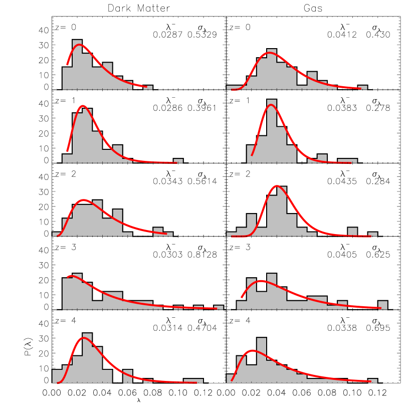
Figure 2.— Distribution of spin parameter $\lambda$ for dark matter (left) and gas (right) for a sample of 41 halos for redshifts ranging from 4 to 0. The solid line is the best fit log-normal distribution as given by Eq. (9). The fit parameters $\bar{\lambda}$ and $\sigma_{\lambda}$ are also labeled on each of the plots.

Figure 3.— $\lambda_{Gas}$ vs $\lambda_{DM}$ for various redshifts. $<\lambda_{gas}/\lambda_{DM}>$ and $<\lambda_{gas}-\lambda_{DM}>$ along with their standard deviations are shown on each plot.

3.2.2 Distribution of Misalignment Angle $\theta$

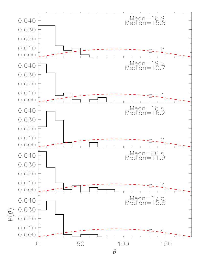
Figure 4.— Distribution of misalignment angle $\theta$ for various redshifts. The dashed line is the expected distribution if the angle is completely random or uncorrelated.

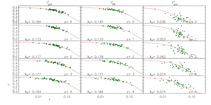
Figure 5.— Counter-rotating fraction $f$ as a function of spin parameter $\lambda$ for various redshifts. Superscript $t$ stands for analysis done with velocities which incorporate random motions and $s$ stands for analysis done with streaming velocities. The solid lines are the fits given by the functional form in Eq. (10). The best value of parameter $\lambda_{0}$ is indicated on each plot.

In LABEL:misaln-dist we show the misalignment angle between the total angular momentum vectors of dark matter and gas for various redshifts. The mean and median values are also shown in each panel. The distribution does not show any significant change with redshift. The mean value $<\theta>$ is around $20$ degrees.

3.2.3 Correlation of $f$ with $\lambda$

As mentioned in LABEL:properties2z3_crop, the fraction of matter with negative angular momentum $f$ is anti-correlated with $\lambda$. We found that the $f$ vs $\lambda$ distribution can be well fit by a function of the form

$$f=1-I_{g}(\frac{\lambda}{\lambda_{0}})\sim 0.5e^{-\lambda/\lambda_{0}}$$ (10)

where $I_{g}(x)=\int_{-\infty}^{x}\frac{e^{-t^{2}/(2\sigma^{2})}}{\sqrt{2\pi}\sigma}dt$ is a Gaussian integral. The results of the applied fit are shown on each plot in LABEL:gl-prop5. The anti-correlation can be described by a single parameter $\lambda_{0}$. For the actual motion of both gas and DM, it is found that $\lambda_{0}$ is around $0.17$ and does not seem to change much except for a decrease in its value at z=0. For streaming motion of gas the parameter $\lambda_{0}$ decreases consistently with decrease in redshift, thus hinting to a systematical change in the distribution of $f_{gas}$ with redshift. Furthermore, the scatter in $f$ vs $\lambda$ plots corresponding to streaming motion of gas ( column 3 LABEL:gl-prop5) is quite large specially at lower redshifts as compared to the plots for broadened motions (column 1 and 2 LABEL:gl-prop5).

3.3. Variation of $<f_{gas}>$ with thermalization of gas

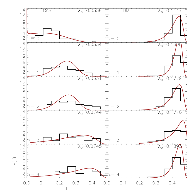
Figure 6.— Distribution of counter-rotating fraction $f$ for gas and dark matter for a sample of 41 halos. The distribution is almost independent of redshift for dark matter while for gas $f$ is lower at lower redshifts. The solid line is the distribution as predicted by Eq. (LABEL:eq:Pf).

In LABEL:predict_fdist the distribution of $f$ is plotted for various redshifts. It can be seen that the distribution for dark matter does not seem to change with redshift, while for gas it shifts towards smaller fractions of negative angular momentum material at lower redshifts. For DM $<f>\sim 0.40$ while for gas $<f>$ decreases from 0.33 to 0.15 monotonically with decrease in redshift (LABEL:thermal1). The kinetic energy of gas particles in SPH simulation, is a combination of translational energy and internal (thermal) energy. The ratio $F_{Tr}=KE_{Tr}/(KE_{Tr}+KE_{Th})$ gives an estimate of thermalization. The lower the $F_{Tr}$ the greater the thermalization. LABEL:thermal1 shows that $<F_{Tr}>$ just like $<f_{gas}>$, also decreases monotonically with decrease of redshift. The correlation of $<F_{Tr}>$ with $<f_{gas}>$ is easy to understand.

Figure 7.— Counter-rotating fractions $<f_{gas}>$ , $<f_{dm}>$ and the fraction of energy for gas in the form of translational motion $<F_{Tr}>$, as a function of redshift. The average is taken over a sample of 41 halos. At lower redshifts the gas gets more and more thermalized, its kinetic energy getting converted into thermal, and this decreases $<f>$.

The dispersion in velocity of particles gives rise to particles with, negative angular momentum. For very small velocity dispersion of particles the fraction with negative angular momentum $f\sim 0$. If velocity dispersion is very large or AM is very small, then $f\sim 0.5$. The SPH particles only have macroscopic flow velocities, the thermal energy is incorporated into U. For DM particles all the energy is in the form of velocities of particles. So $f_{gas}$ is always less than $f_{dm}$. At higher redshift there are more mergers and the gas is more turbulent. As the redshift decreases, the gas undergoes relaxation and kinetic energy of gas gets converted into thermal energy. The velocity dispersion of gas decreases resulting in a decrement of $f_{gas}$. For dark matter $F_{Tr}=1$ and $<f>$ does not show any considerable evolution.

3.4. Effect of numerical resolution

Figure 8.— $f_{gas}$ vs $N_{gas}$ for halos at redshift of $z=0$ simulated at two different resolutions. The fraction $f_{gas}$ does not show any apparent correlation with number of gas particles in the virialized halo indicating that this result is not affected by numerical resolution. The same set of halos re-simulated at $1/8$ times the original resolution also do not show any systematic shift.

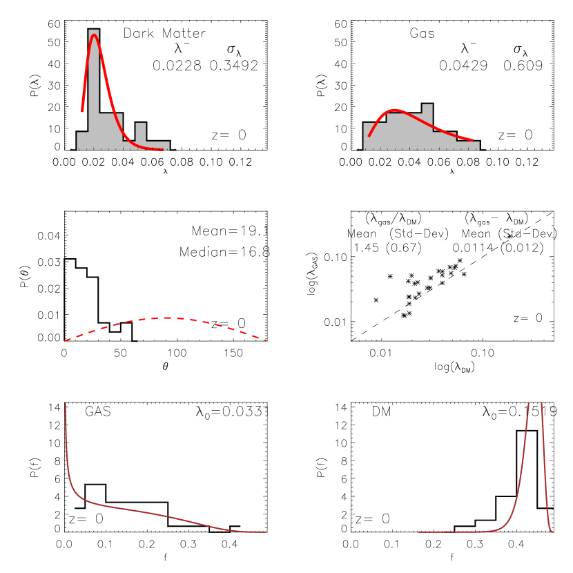
Figure 9.— Various properties of halos and their distributions at $z=0$ from low resolution simulations (1/8 times the normal resolution). A comparison with LABEL:lambda-dist, LABEL:lambdag-lambdad, LABEL:misaln-dist , LABEL:predict_fdist which are the corresponding plots with high resolution simulations shows no difference.

To check whether the numerical resolution has an effect on $f_{gas}$ we plot $f_{gas}$ versus $N$, the number of gas particles in the halo (filled squares in LABEL:f_Vs_N) and find no correlation. To check the effect of numerical resolution in more detail $30$ halos were re-simulated at a lower resolution with $1/8$ times the original number of particles (open triangles in LABEL:f_Vs_N). The values of $f$ do not show any systematic trend with change of resolution. Halos simulated in lower resolution have distributions of $\lambda$ ,$f$ and misalignment angle $\theta$ (LABEL:lowres_prop1) identical to the distributions found in high resolution simulations. So the results shown above are robust to the effect of numerical resolution.

3.5. Evolution of gas particles having negative angular momentum

Figure 10.— The evolution of fraction $f$ of particles with negative angular momentum with scale factor $a$ for various sub-components of gas. Solid line - $f_{global}$ vs $a$, Dotted line(with stars) - $f_{z=0}$ vs $a$ and Dashed line(with squares) - $f_{z=15}$ vs $a$. $f_{global}$ is the fraction of gas with negative angular momentum for the whole halo. $f_{z=0}$ is the corresponding fraction out of a subset of particles that had negative angular momentum at $z=0$. $f_{z=15}$ is the fraction out of a subset of particles that had negative angular momentum at $z=15$.

We investigate whether the gas that ends up with negative angular momentum also had negative angular momentum in the past. We identify a region in past that ends up in the virialized halo at z=0 by simply tracking halo particles at z=0 back in time. We re-center them, and then calculate their angular momentum. The fraction of particles with negative AM at any given stage during the evolution of this Lagrangian volume is a function of redshift so we denote it by $f_{global}(a)$. We identify a subset of particles that were counter rotating at $z=0$, and denote them by subscript $z=0$. The fraction of particles out of this subset that are counter rotating at any given instant is denoted by $f_{z=0}(a)$. Similarly $f_{z=15}(a)$ is the fraction of counter rotating particles out of a subset of particles that were counter rotating at z=15. If the particles with negative angular momentum at $z=0$ were also counter rotating at an earlier epoch, then they would have $f_{z=0}(a)\sim 1$ independent of redshift. Similarly if counter rotating particles at $z=15$ also had negative angular momentum later during their evolution then $f_{z=15}(a)\sim 1$. On the other hand if $f_{z=15}$ or $f_{z=0}\sim f_{global}$ then the particles are just a random subset drawn from the original halo and have no relation with their past or future, respectively.

In LABEL:fvsa_a we have plotted $f_{global}$, $f_{z=0}$ and$f_{z=15}$ as a function of scale factor $a$ of the universe for a randomly selected halo. $f_{z=0}$ and $f_{z=15}$ are both close to 1 at their respective ends but by $z=1$ both fractions have dropped to $f_{global}$ and continue to remain so in respective directions. This suggests that particles that are counter rotating at a given instant will not necessarily counter rotate at a later epoch in future but will instead get mixed up randomly with the remaining portion of the halo.

4. A toy model: Gaussian smearing of ordered velocities (GSOV)

To get a better intuitive understanding of some of the results presented so far, in particular the anti-correlation of $f$ with $\lambda$, we present here a toy model that describes the motion of the particles in the halo. We take a co-ordinate system with the $z$ axis pointing along the direction of the total angular momentum vector. The actual velocity ${\bf u}$ of a particle consists of the ordered motion $v_{o}\hat{\phi}$ (which is motion in circular orbits at a constant speed $v_{o}$), superimposed by random motions ${\bf v_{\sigma}}$. Each component of random motion ${\bf v_{\sigma}}$ is drawn out from a Gaussian distribution with a dispersion $\sigma$. The random motions are assumed to be isotropic. ${\bf u}$ can be written as

$${\bf u} = v_{o}\hat{\phi}+v_{\sigma_{x}}{\bf i}+v_{\sigma_{y}}{\bf j}+v_{\sigma_{z}}{\bf k}$$ (11)

$$= (v_{o}+v_{\sigma_{\phi}})\hat{\phi}+v_{\sigma_{\rho}}\hat{\rho}+v_{\sigma_{z}}{\bf k}$$

According to this model the histogram of $u_{\phi}$ in a halo is given by

$$P(u_{\phi})du_{\phi} = \frac{1}{\sqrt{2\pi}\sigma_{\phi}}e^{-(u_{\phi}-v_{o})^{2}/(2\sigma_{\phi}^{2})}du_{\phi}$$ (12)

In LABEL:gauss_vel1 we have plotted the histogram of $u_{\phi}$ for various halos, for both dark matter and gas. For most halos the $u_{\phi}$ distribution of gas particles can be well described by a Gaussian. Some halos are biased either to right or left, and some show two peaks which can described by two Gaussian functions. A closer examination reveals that these peculiarities are associated with substructure of halos. For dark matter $\sigma$ is large and this washes out any peculiarities that may have been present, consequently no significant deviation from the single Gaussian structure can be observed. Sometimes a slightly sharper peak compared to a Gaussian distribution can be seen indicative of a velocity dispersion that is not strictly isothermal.

In terms of this model the motion within a halo can be described by two parameters $v_{o}$ and $\zeta$ where $\zeta=\frac{\sigma_{\phi}}{v_{o}}$. $\zeta$ is a measure of random motion relative to ordered motion. We calculate $v_{o}$ and $\sigma_{\phi}$ for simulated halos by fitting a Gaussian profile as given by Eq. (12) to the histogram of $u_{\phi}$. LABEL:zeta_dist shows the distribution of $\zeta$ and $v_{o}/V_{v}$ for both gas and DM at $z=0$. $log(\zeta)$ can be fit by a Gaussian both for DM and gas. For gas $\bar{\zeta}\sim 1$ while for DM $\bar{\zeta}\sim 5$.

If the above model of Gaussian smearing is a realistic representation then the fraction of matter with negative angular momentum is simply the probability that $u_{\phi}$ is less than zero, i.e. $v_{\sigma_{\phi}}$ is less than $-v_{o}$ (LABEL:gauss_vel). This can be expressed by an integral

$$f(v_{o},\sigma_{\phi}) = \int_{-\infty}^{-v_{o}}\frac{e^{-v^{2}/(2\sigma_{\phi}^{2})}}{\sqrt{2\pi}\sigma_{\phi}}dv$$ (13)

$$= 0.5[1-Erf(\frac{1}{\sqrt{2}}\frac{v_{o}}{\sigma_{\phi}})]$$

$$= 1-I_{g}(\frac{v_{o}}{\sigma_{\phi}})$$

$$= 1-I_{g}(\frac{1}{\zeta})$$

where $I_{g}(x)=\int_{-\infty}^{x}\frac{e^{-t^{2}/(2\sigma^{2})}}{\sqrt{2\pi}\sigma}dt$ is a Gaussian integral.

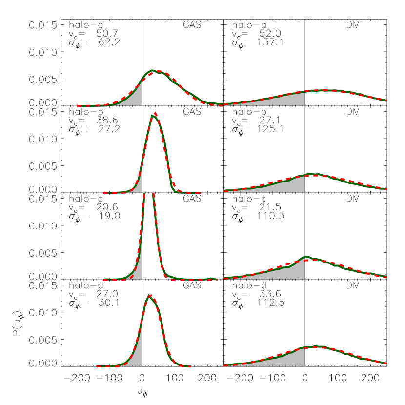
Figure 11.— A plot showing distribution of $u_{\phi}$ for gas and DM for four different halos. Solid line: the histogram for particles in simulation, Dashed line: A Gaussian fit to the above histogram . The shaded region corresponds to particles with negative angular momentum.

Figure 12.— Distribution of parameter $\zeta=\frac{\sigma}{v_{o}}$ and $\frac{v_{o}}{V_{vir}}$ for a sample of 41 halos at z=0. Distributions are roughly log-normal. Gaussian fits are applied and the fit parameters are indicated in upper left and right corners. The position of the peak in normal units is shown below the fit parameters.

$\lambda$ is related to $<j_{z}>$ by

$$\lambda=\frac{<j_{z}>}{\sqrt{2}V_{v}R_{v}}$$ (14)

If we further make the approximation that $<j_{z}/r>=<j_{z}>/<r>$, then using Eq. (14) we can write

$$v_{o} = <u_{\phi}>$$ (15)

$$= <j_{z}/r>$$

$$\sim <j_{z}>/<r>$$

$$\sim \frac{\sqrt{2}\lambda/(V_{v}R_{v})}{<r>}$$

$$\sim \frac{\sqrt{2}\lambda V_{v}}{<r/R_{v}>}$$

This can be used to express $f$ in terms of $\lambda$ as shown below

$$f = 1-I_{g}(\frac{\sqrt{2}\lambda}{<r/R_{v}>(\sigma_{\phi}/V_{v})})$$ (16)

$$= 1-I_{g}(\frac{\sqrt{2}\lambda}{k_{r}k_{\sigma}})$$

where $k_{r}=<r/R_{v}>$ and $k_{\sigma}=(\sigma_{\phi}/V_{v})$ are defined to be two quantities that are constant for a halo. For an NFW halo with concentration parameter $c$

$$k_{r} = <r/R_{v}>$$ (17)

$$= \frac{\int r\rho({\bf r})d^{3}{\bf r}}{\int\rho({\bf r})d^{3}{\bf r}}$$

$$= \frac{\pi}{4}\frac{[1+c-1/(1+c)-2\ln(1+c)]}{c[1/(1+c)-1+\ln(1+c)]}$$

$$= \frac{\pi}{4}f_{1}(c)$$

$$\sim 0.32\ \ \ \ \ \mathrm{for}\ c=10.0$$

We define

$$\lambda_{0}=<k_{r}><k_{\sigma}>/\sqrt{2}$$ (18)

then

$$f = 1-I_{g}(\frac{\lambda}{\lambda_{0}})$$ (19)

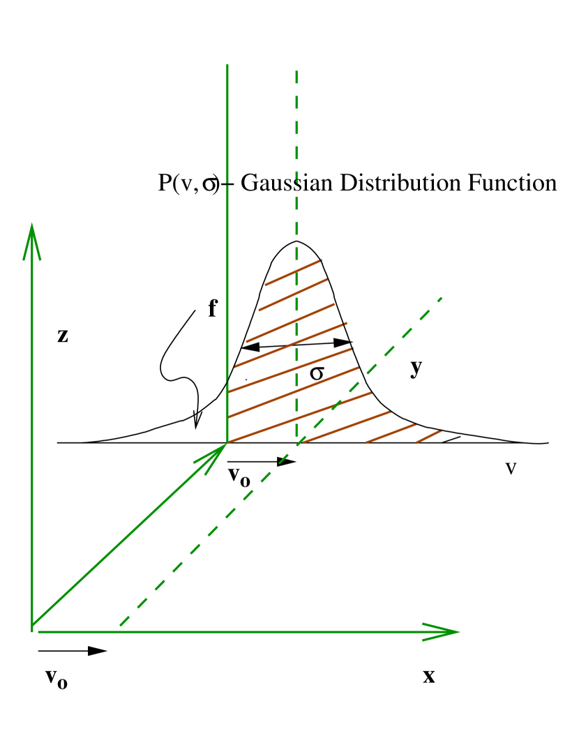
Figure 13.— Dispersion of ordered velocity $v_{o}$ by a Gaussian with width $\sigma$. $P(v,\sigma)=\frac{1}{\sqrt{2\pi}\sigma_{\phi}}e^{-v^{2}/(2\sigma_{\phi}^{2})}$ is the Gaussian distribution function. A particle has negative angular momentum if $v_{\sigma_{\phi}}<-v_{o}$, this is represented by the region under the Gaussian curve which is not shaded.

4.0.1 Anti-correlation of $f$ with $\lambda$

Table 2$k_{r}$ , $k_{\sigma}$ and $\lambda_{0}$ for Gas

	$<k_{r}>$		$<k_{\sigma}>$		$\lambda_{0}$
z	Sim	ENS	Sim	ENS	pred	Sim
0	0.308	0.315	0.163	-	0.036	0.036
1	0.343	0.349	0.181	-	0.044	0.053
2	0.371	0.373	0.210	-	0.055	0.063
3	0.380	0.390	0.217	-	0.058	0.074
4	0.395	0.402	0.213	-	0.059	0.074

Table 3$k_{r}$ , $k_{\sigma}$ and $\lambda_{0}$ for Dark Matter

	$<k_{r}>$		$<k_{\sigma}>$		$\lambda_{0}$
z	Sim	ENS	Sim	ENS	Pred	Sim
0	0.308	0.315	0.632	0.654	0.138	0.145
1	0.350	0.349	0.613	0.605	0.152	0.170
2	0.382	0.373	0.595	0.578	0.161	0.178
3	0.398	0.390	0.590	0.561	0.166	0.177
4	0.409	0.402	0.573	0.551	0.166	0.189

Note. — Sim: simulations, ENS: calculated theoretically by using Eq. (17) and Eq. (LABEL:eq:k_s), $c$ used in calculations is estimated by algorithm given in 2001ApJ...554..114E $\lambda_{0}$ Pred: $\lambda_{0}$ as predicted by the toy model Eq. (18), the values of $<k_{r}>$ and $<k_{\sigma}>$ used are the ones obtained from simulations, $\lambda_{0}$ Sim: $\lambda_{0}$ as obtained by fitting Eq. (19) to the $f$ vs $\lambda$ data from simulations (LABEL:gl-prop5).