The Giant Molecular Cloud associated with RCW 106

We have mapped the dust continuum emission from the molecular cloud covering a region of 28 pc$\times$94 pc associated with the well-known H ii region RCW 106 at 1.2 mm using SIMBA on SEST. The observations, having an HPBW of 24″ (0.4 pc), reveal 95 clumps, of which about 50% have MSX associations and only 20% have IRAS associations. Owing to their higher sensitivity to colder dust and higher angular resolution the present observations identify new emission features and also show that most of the IRAS sources in this region consist of multiple dust emission peaks. The detected millimeter sources (MMS) include on one end the exotic MMS5 (associated with IRAS 16183-4958, one of the brightest infrared sources in our Galaxy) and the bright (and presumably cold) source MMS54, with no IRAS or MSX associations on the other end. Around 10% of the sources are associated with signposts of high mass star formation activity. Assuming a uniform dust temperature of 20 K we estimate the total mass of the GMC associated with RCW 106 to be $\sim 10^{5}$ M_⊙. The constituent millimeter clumps cover a range of masses and radii between 40 to $10^{4}$ M_⊙ and 0.3 to 1.9 pc. Densities of the clumps range between (0.5-6) 10⁴ cm^-3. We have decomposed the continuum emission into Gaussian and arbitrary shaped clumps using the two independent structure analysis tools gaussclumps and clumpfind respectively. The clump mass spectrum was found to have an index $\alpha$ of $1.6\pm 0.3$, independent of the decomposition algorithm used. The index of the mass spectrum for the mass and length scales covered here are consistent with results derived from large scale CO observations.

1 Introduction

Massive stars are believed to form in clusters within molecular cloud complexes. Owing to their occurrence in more distant crowded stellar clusters, shorter formation timescales and formation in regions of high visual extinction, the formation of massive stars is still poorly understood. Dense, cool molecular gas and dust cocoons enshroud massive protostars and account for most of the extinction toward these regions. The extinction is generally so high that a massive protostar cannot be directly observed even at the K band (2.2 $\mu$m). Watson et al. (1997) succeeded in one of the rare direct observations of the ionizing star in K band for the UCH ii region G29.96-0.02. Optically thin millimeter and submillimeter continuum emission from dust cocoons shrouding the sites of massive star formation is a valuable probe of molecular cloud structure. Owing to the recent developments in the detection techniques at millimeter and sub-millimeter wavelengths, large continuum maps essential for deriving a census of dust emission peaks arising from the deeply embedded phases of star formation are becoming available (Johnstone et al. 2000; Motte et al. 2001, 2003).

RCW 106 was discovered by Rodgers, Campbell, & Whiteoak (1960) in a survey of H$\alpha$ line emission of the southern Galactic plane. The Giant Molecular Cloud (GMC) associated with RCW 106, was first detected by Gillespie et al. (1977) during observations of the molecular clouds associated with southern Galactic H ii regions in the J=1-0 transition of CO. Radio continuum mapping observations at 408 MHz and 5 GHz by Goss & Shaver (1970) detected a number of bright H ii regions occurring along a line almost parallel to the Galactic plane. IRAS observations have subsequently shown all of these H ii regions to be bright infrared sources. The GMC is located at a distance of 3.6 kpc (Lockman 1979) covering an area of 70′ $\times$15′ between $l$=332.5 to 333.7 and appears as a large complex of bright mid-infrared sources in the Midcourse Space Experiment (MSX) images between 8 and 21 $\mu$m (20″ resolution). The region contains one of the brightest infrared sources in our Galaxy (Becklin et al. 1973), IRAS 16183-4958, which harbors the H ii region G333.6-0.22. In addition to the IRAS maps at the mid and far-infrared wavebands, far-infrared (FIR) balloon-borne observations (1′ angular resolution) of the dust continuum at 150 and 210 $\mu$m (Karnik et al. 2001) identified 23 emission peaks with dust temperatures between 20 and 40 K. Largescale CO(1-0) observations by Bronfman et al. (1989) with an angular resolution of 9′ obtained a global view of the molecular gas distribution in this region. However most of the remaining spectroscopic observations toward this GMC are primarily pointed mode observations of the emissions of the lines of CO (Gillespie et al. 1977; Brand et al. 1984), CS (Gardner & Whiteoak 1978; Bronfman et al. 1996), H₂CO (Gardner & Whiteoak 1984), NH₃(Batchelor et al. 1977), H₂O, OH and methanol masers (Braz & Epchtein 1983; Caswell 1997; Walsh, Hyland, Robinson, & Burton 1997) toward predetected H ii regions and IRAS sources. These observations suggest ongoing high-mass star formation activity and enhanced density cores associated with most of the strong emission peaks. This region will also be observed as a part of the Galactic Legacy Infrared Mid-Plane Survey Extraordinaire (GLIMPSE), a Spitzer Legacy Science Program (Benjamin et al. 2003) at 3.6, 4.5, 5.8, and 8.0 $\mu$m using the Infrared Array Camera (IRAC).

In this paper we present the first sensitive, large-scale continuum survey of the RCW 106 region at millimeter wavelengths. We have used the 1.2 mm observations to identify $95$ clumps, about half of which have MSX counterparts. We discuss association of these clumps with sources detected in MSX and IRAS surveys in particular. We have used methods based on clumpfind (Williams & Blitz 1993; Williams et al. 1994) and gaussclumps (Stutzki & Güsten 1990) to derive the clump mass distribution in this region.

2 Observations and data reduction

The 1.2 mm continuum observations were carried out with the 37 channel bolometer array SIMBA (SEST Imaging Bolometer Array) at the SEST (Swedish-ESO Submillimeter Telescope) on La Silla, Chile during the night from July 4 to 5, 2002. A mosaic covering approximately $1600$″$\times$5400″ ($\alpha\times\delta$) was observed using the fast scanning method. The mapped region extends over 28 pc$\times$94 pc. Altogether 8 individual maps were used to construct the large mosaic and the total observing time was about 9.5 hours. The zenith opacity during the observation, measured using skydips, ranged between 0.209 and 0.385. For all but the two submaps at the top, two coverages were possible, resulting in differences in the noise levels between the northernmost part of the map and the rest of it. The residual noise in the final co-added mosaic is 23 mJy/beam for most of the southern part of the mosaic and is around 50 mJy/beam for the northernmost part. Uranus was mapped for calibration purposes and a calibration accuracy of 15% was achieved. The HPBW for these observations was 24″.

All data were reduced and analyzed using MOPSI according to the instructions of the SIMBA Observer’s Handbook (2002) and also using methods described by Chini et al. (2003). Figure 1 shows the 1.2 mm dust continuum emission from the region associated with RCW 106 as observed by SIMBA, together with the associated IRAS point sources.

Figure 1: The 1.2 mm mosaic of the star forming regions around RCW 106 observed with SIMBA. The typical 1$\sigma$ rms noise is 23 mJy/beam. The contours correspond to 0.1, 0.2, 0.5, 1, 2, 4, 10, 12, 15, 20, and 40 Jy/beam. All associated IRAS point sources are also indicated in the plot.The mapped region extends over 28 pc$\times$94 pc. Also shown in the plot is the SIMBA beam.

3 Results

To locate and measure the properties of dust emission peaks or “clumps” as we shall refer to them in this paper (see Section 3.4), we have used an automated procedure based on a two-dimensional variant of the clump-finding algorithm, clumpfind (Williams et al. 1994). The clumps so identified may have any arbitrary shape, so that the procedure gives results similar to what an inspection by eye would have done but being automated, has far better accuracy. We further imposed the conditions that in order to be identified as a genuine sub-mm source, a clump must have (1) a deconvolved size larger than 50% of the HPBW (24″) and (2) an S/N ratio greater than 5. Table The Giant Molecular Cloud associated with RCW 106 lists the positions, peak intensities, integrated intensities, derived physical properties (size, mass and density) of the 95 clumps that have been detected at 1.2 mm.

3.1 Overview of mm sources

To obtain a first estimate of the nature of the sources detected at 1.2 mm we have derived associations of these sources with existing MSX and IRAS point sources. We have associated a millimeter source with an MSX (or IRAS or FIR) source if the MSX (or IRAS or FIR) source lies within a radius of 40″ (90″ or 60 ″) from the millimeter source. We have also identified different signposts of massive star formation viz., H ii regions, masers (H₂O, OH, methanol etc) associated with the clumps. In addition, the MSX point sources for which the logarithm of the ratio of the Band A (8 $\mu$m) to the Band E (21 $\mu$m) flux densities, $log(S_{8}/S_{21})\geq 0.57$, are identified as candidates for UCH ii regions (R. Simon, $priv.\leavevmode\nobreak\ communication$). This is a direct extension of the Wood-Churchwell criterion (Wood & Churchwell et al. 1989) for identifying UCH ii regions based on the the IRAS 12 and 25 $\mu$m flux densities. Figures 2, 3 and 4 show overlays of the MSX (greyscale) 8 $\mu$m image with the SIMBA contours, with the mm-sources marked together with all MSX-UCH ii candidates in the region. We note that this method of deriving associations could be severely affected by the differences in the resolutions and sensitivities of the different observations under consideration. Following this method, we identify two main types of clumps:

Type A : Clumps with an infrared (IRAS or MSX or FIR) association. Table 1 lists the 46 type A clumps together with the associated IRAS and MSX point sources, H ii regions, MSX-UCHII candidates and H₂O, methanol or OH masers. Owing to the higher angular resolution of the 1.2 mm dataset presented here in contrast to the IRAS beamsizes, on several occasions a single IRAS source is associated with two or more clumps. All sources except five (MMS40, MMS52, MMS61, MMS63, MMS80) have MSX associations. Almost all clumps with MSX and IRAS associations are also identified as candidates for MSX UCH ii regions. Only 7 type A clumps are found to have H ii regions associated with them and only 5 of them (MMS5, MMS9, MMS39/40, MMS68 and MMS84) have associated maser activities. MMS 54, having only a FIR association, has a methanol maser associated with it. Type A sources with associated H ii regions are thus the more evolved, massive star-forming clumps of this region.

Type B : The remaining 49 clumps with no infrared associations. These are pure sub-mm sources, some of which are mass or size-wise no different from the Type A sources (see Section 3.3).

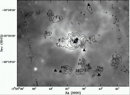
Figure 2: Contours of 1.2 mm dust continuum overlayed on the MSX 8 $\mu$m image for the northernmost sub-region. The rms noise for the map is 50 mJy/beam and the contours are 0.2, 0.5, 1.0, 1.5, 2.5, 5.0 Jy/beam and 10 to 40 Jy/beam in steps of 5. The millimeter clumps ($+$) and MSX-UCH ii candidates (filled triangles) are marked.

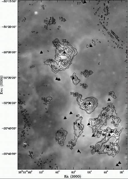
Figure 3: Same as in Figure 2 only for the middle part of the mapped region. The contours are at 0.1, 0.2, 0.5, 1, 1.5, 2.5, 5 and 8.5 Jy/beam.

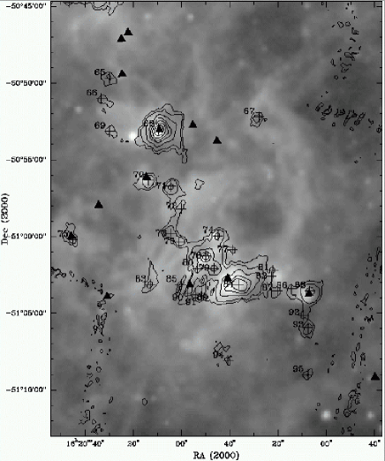
Figure 4: Same as in Figure 3 only for the southernmost part of the mapped region. The contours are at for 0.1, 0.2, 0.5, 1, 1.5, 2.5, 5 10 and 12 Jy/beam.

3.2 Mass

Table The Giant Molecular Cloud associated with RCW 106 also presents the masses of the clumps ($M_{\rm clump}$) derived from their total integrated flux densities ($F_{\nu}$) using the following relationship:

$$M_{\rm gas}\leavevmode\nobreak\ =\leavevmode\nobreak\ \frac{F_{\nu}D^{2}}{\kappa_{\nu}B_{\nu}(T_{\rm dust})}.$$ (1)

This equation is valid since dust emission at 1.2 mm is optically thin.

In equation 1, $B_{\nu}(T_{\rm dust})$ is the Planck function at the dust temperature $T_{\rm dust}$, $\kappa_{\nu}$ is the dust mass opacity coefficient, $D$ is the distance. In the absence of complementary continuum data, we generally assume a dust temperature of 20 K which is typically found in star forming cloud complexes (Johnstone et al. 2000; Motte et al. 2003, e.g.). However for the clumps with associated H ii regions we have assumed $T_{\rm dust}$ to be 40 K (Karnik et al. 2001). For the dust mass opacity coefficient we adopt the value of $\kappa_{230GHz}\leavevmode\nobreak\ =\leavevmode\nobreak\ 0.005$ cm² g^-1 Preibisch et al. (1993) assuming a gas-to-dust mass ratio of 100, and $\kappa_{\nu}$ = $\kappa_{230GHz}$($\nu$/230GHz)^β, with $\beta$ = 2. Assuming a uniform dust temperature of 20 K, the total mass of the region is estimated to be $10^{5}$ M_⊙.

A few additional details about the calculation of the mass:

(1) Given the large population of UC-H ii candidates in the region, 1.2 mm continuum emission observed with SIMBA is most likely to be contaminated by the free-free emission from the H ii regions. However as mentioned earlier, no radio continuum image of comparable angular resolution is available for the entire region. For the clumps with associated H ii regions the contribution of the free-free emission from the gas nevertheless has been estimated using the available 5 GHz flux densities (Haynes, Caswell, & Simons 1979) and a power law dependence of S${}_{\nu}\sim\nu^{-0.1}$, for optically thin free-free emission. The contribution varies between 4 and 36% (see Table The Giant Molecular Cloud associated with RCW 106). For the clumps for which the radio continuum flux densities were not available, despite their association with an H ii region, we have assumed a constant 20% contribution to the flux densities at 1.2 mm.

(2) Two other sources of uncertainty in converting the observed flux density at 1.2 mm into gas mass are (a) the dust to gas mass ratio which typically ranges between 100 and 150 and (b) the dust mass opacity coefficient, which ranges between 0.003 (diffuse ISM) up to 0.02 cm² g^-1 (Krügel & Siebenmorgen 1994) for dense protostellar environments, depending on the size and structure of the dust grains.

3.3 Sizes & densities

At a distance of 3.6 kpc the HPBW of 24″ of SIMBA corresponds to a diameter of 0.42 pc. The radii of the clumps identified by clumpfind range between the resolution limit to as large as 1.9 pc, with a substantial fraction having radii larger than 0.6 pc. Thus most of these clumps are of the size of star forming regions, rather than the innermost star forming cores typically of 0.01 to 0.1 pc size which have been dealt with in similar mm/sub-mm continuum studies of regions like $\rho$ Ophiuchi, Orion B, W 43, IC 5146 etc. (Motte et al. 1998; Johnstone et al. 2000; Motte et al. 2003; Kramer et al. 2003).

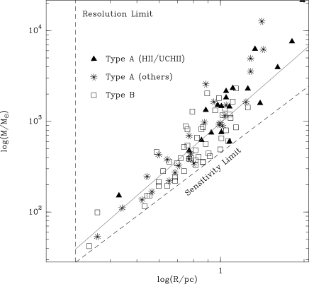
Figure 5: Plot of mass as a function of the radius (convolved with the beam) for all detected clumps. The dashed vertical line corresponds to the minimum size that a clump may have (resolution limit) and the other dashed line shows the minimum mass that a clump must have in order to be 1$\sigma$ above the mass detection limit. The sensitivity limit corresponds to M$\propto$R². Also shown is the M$\propto$R^2.3 as found in CO observations (Heithausen et al. 1998), extrapolated to masses higher than 100 M_⊙.

Figure 5 shows a log-log plot of the estimated mass as a function of the radii for all the 95 millimeter clumps in this region. Since the clumps are not point sources, the completeness limit, measured in total flux or mass depends on both the range of object sizes and the surface brightness profiles. This holds for all surveys that attempt to measure the integrated flux from extended objects. Figure 5 shows that most of the more massive and larger clumps also belong to Type A and are either H ii regions or candidates for UC-H ii regions. Figure 5 does not show any clear distinction between the two types of clumps. There appears to be a distinct mass-to-radius correlation for all the clumps, although part of it probably arises from the resolution and sensitivity limits. The continuous line shows the mass to radius correlation (M$\propto$R^2.3) seen in CO clumps (Heithausen et al. 1998) for $0.01<R/pc<10$ and $10^{-4}<$M/M_⊙$<10^{2}$. For comparison, the Type A clumps show a M$\propto$R^2.8±0.3 correlation, whereas the Type B clumps exhibit a M$\propto$R^2.3±0.2 correlation. This implies that within the uncertainties the mass-radius relation for all types of clumps agree well with the result from Heithausen et al. (1998) as well as the sensitivity limit.

The slope found for the dense, small prestellar objects studied by e.g. Motte et al. (2001), is much shallower: $M\propto\,R^{1.1}$ though this relation may likewise be affected by the size-dependent detection thresholds. However, as pointed out by Motte et al. (2001) a linear relation is expected for self-gravitating isothermal condensations.

Based on the calculated mass and derived sizes, in Table The Giant Molecular Cloud associated with RCW 106 we also present the estimated densities of the clumps. We find that the clumps have moderate densities ($\sim 10^{4}$ cm^-3) spread over a rather narrow range. The densities are similar to those observed in the dust continuum study by Kerton et al. (2001) as well as the typical densities found in CO emission studies. The estimated densities also show that the sources under consideration here are quite different from the high density ($\sim 10^{6}$ cm^-3) condensations which are considered to be prestellar candidates (Motte et al. 1998).

3.4 Nature of the mm sources

Blitz (1993) proposed an operational categorization for structures of different spatial scales seen in the ISM. In this scheme three types of structures are defined, viz., clouds, clumps and cores. Clouds are structures with masses $>10^{4}$ M_⊙ and cores are regions out of which single stars (or binary systems) form with masses $\leq 10$ M_⊙ and sizes $\leq 0.1$ pc. Clumps correspond to structures with masses and sizes intermediate between clouds and cores, from which stellar clusters are formed. The millimeter sources detected around RCW 106 have radii between 0.3 and 1.9 pc and have masses between 40 and $10^{4}$ M_⊙. Thus we refer to these sources as clumps and the entire region mapped with a mass of $\sim 10^{5}$ M_⊙ as Giant Molecular Cloud (GMC).

Given the limitations involved in associating the clumps with the radio observations detecting various signposts of star forming activities (viz., H ii regions, masers), the evolutionary stages of the clumps identified here are not accurate. The case of MMS54 is an apt example. While its fainter companion MMS57 has an MSX counterpart, the stronger millimeter source MMS54 has no IRAS or MSX associations, but was detected both at 150 and 210 $\mu$m by Karnik et al. (2001) and has an associated methanol maser (Ellingsen et al. 1996, observed with an angular resolution of 4′). This definitely suggests that MMS54 shows early signs of massive star formation and demands further high angular resolution sub-mm dust continuum observations to characterize its nature.

Broadly, we propose the following evolutionary stages for the clumps:

(1) Type A clumps with associated H ii regions (and some of them with maser activities as well) are the most evolved high mass star forming regions.

(2) Type A clumps which are candidates for MSX-UCH ii regions (refer to Section 3.1 for the criterion) are high mass star forming regions, less evolved than those in (1).

(3) Type A clumps which have only infrared associations and do not qualify as UCH ii candidates are possible sites of low mass star formation at early stages of evolution.

(4) The purely mm clumps (Type B) are cold condensations, which given their densities are either prestellar or transient features of the molecular cloud.

Most of the existing spectroscopic observations are aimed at the sources (belonging to category (1) of Type A) that are bonafide massive star forming regions. Thus for the newly detected clumps there are no available spectroscopic observations which may be used to estimate their gravitational stability and hence help to judge the potential of these clumps to be prestellar objects.

4 Clump mass distribution

Molecular cloud structure can be mapped via mm spectroscopy of molecular lines, continuum (sub)millimeter emission from dust or stellar NIR absorption by dust. The first method gives kinematical as well as spatial information and results in a three dimensional cube of data, whereas the latter two result in two dimensional datasets. We use the second method to derive information about the structure of the molecular cloud around the RCW 106 region.

For this purpose we have made use of the two most direct structure analysis tools, viz., clumpfind (Williams et al. 1994) and gaussclumps (Stutzki & Güsten 1990; Kramer et al. 1998) both of which decompose the observed emission into discrete clumps. The masses derived using clumpfind are already presented in Table The Giant Molecular Cloud associated with RCW 106. We have also used gaussclumps which follows a completely different clump identification and extraction algorithm. In contrast to clumpfind, the gaussclumps algorithm iteratively deconvolves the observed emission into Gaussian shaped clumps. Though this algorithm was originally written to decompose 3-dimensional molecular line data sets, it can also be applied to slightly adapted continuum data without modification of the code. Motte et al. (2003) already used this method to analyze a continuum data set of W43.

For both clumpfind and gaussclumps, we have selected only those clumps that have deconvolved sizes larger than 50% of the spatial resolution of the SIMBA data for further analysis. This discards the very small clumps which contribute only a tiny fraction to the total mass.

The masses of the identified clumps range between 40 and $10^{4}$ M_⊙ (Table 2). It is worth noting that particularly for the low mass clumps there is no one-to-one correspondence between positions and masses of individual clumps found by gaussclumps and clumpfind. The gaussclumps algorithm decomposes a larger fraction of the total flux into clumps (Table 2) and thus finds a larger number of clumps. However we point out here that the purpose of this structure analysis and construction of the mass spectrum is to obtain an overview of the statistical properties of the clump ensemble. Thus, we have used all clumps regardless of their nature and/or evolutionary stages to build up the mass spectrum.

Figure 6 shows the resulting distributions in a log-log plot of the number of clumps found per mass interval. We find that the clump mass distributions have similar shapes. The slope of the distribution flattens when going from the clumps of $\sim 10^{4}$ M_⊙ to clumps of $\sim 10^{3}$ M_⊙. At smaller masses of $\sim 190$ M_⊙ corresponding to the $10\sigma$ mass at $T_{\rm dust}=20$ K, the distributions are almost flat. There is a sharp turnover of the spectra at still lower masses. No clumps are found beyond the minimum $1\sigma$ mass. The turnover at masses of less than the $10\sigma$ mass has often been found in mass spectra created from CO surveys. Heithausen et al. (1998) showed that this turnover is not an intrinsic property of the clump distribution but rather due to the finite resolutions and the finite sensitivity. Observations at higher resolutions, show a smooth continuation of the mass spectra without any change in slope. A linear least squares fit to the clump distribution $dN/dM\propto M^{-\alpha}$ for clumps with $M>10\sigma$, results in linear correlation coefficients between 80 and 90% and spectral indices $\alpha$ of between 1.7 and 1.6. Both spectra yield the same index within the standard deviation of $0.3$.

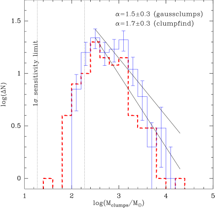
Figure 6: The mass spectrum for the clumps identified using clumpfind (dashed histogram) and gaussclumps (drawn histogram) respectively. Error bars represent the standard deviation of a Poisson distribution $\sqrt{\Delta N}$ and are only drawn for one spectrum for clearness. The dashed vertical line indicates the $1\sigma$ (=19M_⊙) and $10\sigma$ masses given by the average noise level of the map of 50 mJy/beam, the beam size ($24^{\prime\prime}$, i.e. 0.42 pc), and assuming $T_{\rm dust}=20$ K.

As pointed out in Section 3.4, star forming cores are not detected by our survey. This is an important aspect to keep in mind while comparing the results of the structure analysis presented here with the results of dust continuum and molecular line studies.

Table 2 compares the properties of the clump ensemble obtained for RCW 106 with those of other dust continuum mapping observations studying the fragmentation of the clouds. We restrict the table only to those studies which consider clumps that are more massive than stars and more extended than the prestellar cores considered e.g. by Motte et al. (1998). Interestingly, the spectral indices of the clump mass distributions from these studies lie at $\sim 1.6$.

This is in contrast to the recent dust continuum maps obtained at high resolution for the nearby clouds $\rho$Ophiuchus, Serpens, and NGC 2068/71 (Motte et al. 1998; Testi & Sargent 1998; Johnstone et al. 2000; Motte et al. 2001). The properties of the resulting clump distributions have been compiled by Motte & André (2001). In these studies, clumps have masses down to 0.02 M_⊙, sizes less than 0.05 pc ($\leq 10\,000$ AU), and typical densities of $10^{6}$ cm^-3. These starless and gravitationally bound clumps are therefore good candidates for being the progenitors of protostars. The above studies show a common spectral index of the clump mass distribution of $\sim 2.3$. There are only a few exceptions: the studies of Sandell et al. (2001) and Coppin et al. (2000) show indices of $\sim 1.5$.

A spectral index of $\sim 2.3$ matches with the Salpeter IMF (Salpeter 1955) which is thought to hold for stars $>1$M _⊙ (Kroupa et al. 1993; Scalo 1998). There are indications in $\rho$Oph that at still lower masses, the dust continuum mass spectrum flattens out, as does the stellar IMF.

Interestingly, the mass spectrum found here for $40<$M/M_⊙$<10^{4}$ is similar within the uncertainties to the mass spectra derived from Galactic large-scale CO maps covering the mass range $10^{-4}<$M/M_⊙$<10^{4}$ (e.g. Heyer et al. 2001; Simon et al. 2000; Kramer et al. 1998, and references therein) all of which agree with $1.5<\alpha<1.8$. In a recent study of CO in the Antennae galaxies (NGC 4038/4039), Wilson et al. (2003) found again similar index of 1.4 for a mass range from $5\,10^{6}$ to $9\,10^{8}$M_⊙ of the entire cloud complex using clumpfind.

Thus the spectral index of the clump mass distribution found here is independent of the algorithm used and is consistent with both dust continuum and CO mapping studies which probe structures of densities $\sim 10^{3}-10^{4}$ cm^-3 as we find in RCW 106. Spectral line maps at high spatial resolutions are needed to examine the stability of these clumps and find out whether they are gravitationally bound or are transient features of the turbulent clouds.

5 Summary

The 1.2 mm dust continuum emission from the GMC associated with the well-known H ii region RCW 106 has been mapped at an angular resolution of 24″ using SIMBA. In all, 95 mm clumps have been identified, more than half of which are associated with pre-detected IR(MSX or IRAS) point sources. The region contains a number of dense massive star forming clumps which are recognized as candidates for UCH ii regions and are bright in the far-infrared and millimeter wavelengths. There exist a large number of molecular condensations which are only bright in the millimeter wavelengths and have no IR associations. MMS54 has no MSX or IRAS associations but was detected in the FIR by Karnik et al. (2001) and has an associated methanol maser; it is a strong candidate for a star forming region at a very early stage of evolution. The continuum emission has been resolved in to Gaussian and arbitrary-shaped clumps using the two independent structure decomposition tools gaussclumps and clumpfind respectively. The masses of these clumps cover a wide range between 40 to $10^{4}$ M_⊙, suggesting that while the entire region is similar to a GMC, the sources detected are more like star forming regions (protoclusters) and not cores which would give rise to individual stars. The distribution of the clump mass was found to have a spectral index $\alpha$ of $1.6\pm 0.3$, independent of the decomposition algorithm used. The spectral index of their distributions match well with those observed in CO observations covering the same mass range.

The higher angular resolution of this survey in contrast to the previous IRAS and far-infrared observations allows the identification of a number of clumps which are potentially interesting for further detailed continuum observations in the far-infrared and sub-mm as well as spectroscopic observations. Owing to the southern location of the region, ground-based observations will have to wait for the upcoming telescopes like APEX and later ALMA.

[x]lllrrrrc Observed and derived parameters of the millimeter sources detected in the RCW 106 complex. Dust masses have been calculated for T_dust = 20 K and an emissivity $\beta=2$. Column (5) gives the clump radii (convolved with the beam). Estimated free-free contribution to the 1.2 mm flux densities from the H ii regions are ¹ 23%, ² 20%, ³ 36%, ⁴ 12%, ⁵ 4%, ⁶ 18%. The masses for these sources are calculated assuming a temperature of 40 K.
Source RA(2000) Dec(2000) F_peak Radius F_ν Mass n${}_{\mathrm{H}_{2}}$
mJy/beam pc Jy M_⊙  10⁴ cm^-3
continued
Source RA(2000) Dec(2000) F_peak Radius F_ν Mass n${}_{\mathrm{H}_{2}}$
mJy/beam pc Jy M_⊙  10⁴ cm^-3
MMS1 16:22:39.8 -50:01:00 828 0.81 2.5 956 1.74
MMS2 16:22:28.9 -50:01:41 585 0.90 2.9 1097 1.45
MMS3 16:22:41.6 -50:04:36 375 0.60 1.0 376 1.68
MMS4 16:21:49.3 -50:05:43 379 0.63 1.3 500 1.93
MMS5 16:22:10.1 -50:06:06 40013¹ 1.88 129.5 15936 5.44
MMS6 16:22:25.9 -50:06:04 370 0.89 2.7 1003 1.37
MMS7 16:22:29.2 -50:06:52 430 0.89 2.2 834 1.14
MMS8 16:22:01.1 -50:09:59 502 0.51 0.7 274 2.00
MMS9 16:21:20.3 -50:09:45 4392² 0.83 8.6 1096 5.44
MMS10 16:22:01.2 -50:10:31 475 0.47 0.8 308 2.87
MMS11 16:21:55.4 -50:10:54 356 0.49 0.5 203 1.67
MMS12 16:21:38.8 -50:11:20 258 0.47 0.4 154 1.43
MMS13 16:22:22.1 -50:11:17 775 0.65 2.5 928 3.26
MMS14 16:21:52.9 -50:11:19 273 0.64 0.8 285 1.05
MMS15 16:21:40.5 -50:11:51 546 0.93 2.8 1052 1.26
MMS16 16:22:04.6 -50:11:58 1015 0.80 3.2 1187 2.24
MMS17 16:21:08.0 -50:15:14 578 0.32 0.3 109 3.21
MMS18 16:21:32.3 -50:18:49 195 0.51 0.4 139 1.01
MMS19 16:21:44.9 -50:18:48 183 0.41 0.2 83 1.16
MMS20 16:21:46.6 -50:19:03 178 0.24 0.1 30 2.10
MMS21 16:21:49.9 -50:19:03 161 0.55 0.4 158 0.92
MMS22 16:21:50.8 -50:19:27 198 0.72 0.7 259 0.67
MMS23 16:21:28.4 -50:23:12 163 0.47 0.4 139 1.29
MMS24 16:21:40.9 -50:23:11 564 0.62 1.6 590 2.39
MMS25 16:21:39.3 -50:23:53 761 0.84 3.5 1311 2.14
MMS26 16:21:27.6 -50:24:56 1460³ 1.25 11.2 1151 1.34
MMS27 16:21:32.6 -50:25:20 3672³ 0.96 16.5 1692 4.34
MMS28 16:21:45.3 -50:27:04 375 1.09 3.1 1183 0.88
MMS29 16:21:32.7 -50:27:12 6502 1.27 24.7 9281 4.38
MMS30 16:21:42.9 -50:28:15 524 0.96 3.2 1198 1.31
MMS31 16:21:00.9 -50:29:15 308 0.58 0.8 282 1.40
MMS32 16:21:06.0 -50:29:39 319 0.67 0.9 346 1.11
MMS33 16:21:18.6 -50:30:25 1095 0.90 3.5 1325 1.76
MMS34 16:21:06.9 -50:31:55 282 0.56 0.7 248 1.36
MMS35 16:21:18.8 -50:33:37 190 0.43 0.3 109 1.32
MMS36 16:20:31.8 -50:33:48 225 0.57 0.6 233 1.22
MMS37 16:21:13.8 -50:33:45 451 0.72 1.7 624 1.62
MMS38 16:21:54.9 -50:34:40 283 0.99 1.6 620 0.62
MMS39 16:21:03.7 -50:35:23 8925⁴ 1.19 32.6 4584 6.18
MMS40 16:21:01.2 -50:35:54 4054⁴ 1.14 18.3 2580 3.95
MMS41 16:20:31.8 -50:36:04 151 0.67 0.7 267 0.86
MMS42 16:20:39.4 -50:36:36 804 0.99 4.5 1675 1.67
MMS43 16:20:38.5 -50:37:41 369 0.46 0.9 331 3.29
MMS44 16:20:40.2 -50:37:56 373 0.71 1.6 593 1.60
MMS45 16:21:12.1 -50:38:02 173 0.40 0.3 98 1.48
MMS46 16:20:30.1 -50:38:12 479 0.87 2.3 849 1.25
MMS47 16:20:49.5 -50:38:43 3322 1.29 12.1 4530 2.04
MMS48 16:20:28.4 -50:39:24 298 0.74 1.1 406 0.97
MMS49 16:21:15.6 -50:39:29 763 0.74 2.6 965 2.30
MMS50 16:21:13.9 -50:39:45 762 1.11 4.4 1664 1.18
MMS51 16:20:52.1 -50:40:51 348 1.11 2.7 1029 0.73
MMS52 16:20:29.4 -50:41:00 741² 0.93 3.4 431 1.52
MMS53 16:20:36.9 -50:41:00 1268² 0.71 3.5 448 3.55
MMS54 16:21:35.8 -50:41:11 2765 1.14 9.6 3598 2.35
MMS55 16:20:44.5 -50:41:23 173 0.55 0.5 173 1.00
MMS56 16:20:39.4 -50:41:48 968² 0.86 4.3 548 2.45
MMS57 16:21:37.6 -50:42:49 359 0.85 1.8 691 1.09
MMS58 16:21:21.6 -50:43:22 326 0.90 1.5 575 0.76
MMS59 16:20:30.3 -50:43:33 326 0.84 1.8 665 1.08
MMS60 16:21:24.2 -50:44:01 153 0.26 0.1 38 2.09
MMS61 16:20:37.8 -50:44:04 893 0.90 4.2 1563 2.07
MMS62 16:20:54.7 -50:44:11 426 0.93 2.3 860 1.03
MMS63 16:20:28.6 -50:44:44 258 0.87 1.7 642 0.94
MMS64 16:20:48.8 -50:44:59 160 0.60 0.5 203 0.91
MMS65 16:20:32.0 -50:49:56 233 0.69 0.8 293 0.86
MMS66 16:20:35.4 -50:51:17 159 0.67 0.6 237 0.76
MMS67 16:19:30.4 -50:52:32 328 0.63 0.7 278 1.07
MMS68 16:20:11.9 -50:53:17 12460⁵ 1.70 36.1 5548 2.56
MMS69 16:20:32.1 -50:53:24 170 0.72 0.7 255 0.66
MMS70 16:20:16.1 -50:56:38 482 0.78 1.4 541 1.10
MMS71 16:20:06.8 -50:57:02 603 0.94 2.1 789 0.92
MMS72 16:20:02.6 -50:58:30 155 0.92 1.2 436 0.54
MMS73 16:20:06.8 -51:00:06 439 0.62 1.0 391 1.58
MMS74 16:19:47.4 -51:00:15 662 0.73 1.9 702 1.74
MMS75 16:20:47.6 -51:00:27 417 0.63 0.9 342 1.32
MMS76 16:20:03.5 -51:00:38 424 0.52 0.7 259 1.78
MMS77 16:19:41.4 -51:01:11 176 0.77 0.8 297 0.63
MMS78 16:19:52.5 -51:01:35 1905 0.74 5.0 1867 4.45
MMS79 16:19:49.1 -51:02:24 1331 0.75 3.9 1476 3.38
MMS80 16:19:55.8 -51:02:23 670 0.61 1.7 639 2.72
MMS81 16:19:24.4 -51:02:33 154 0.66 0.7 248 0.83
MMS82 16:19:25.3 -51:02:56 164 0.44 0.3 120 1.36
MMS83 16:20:15.4 -51:03:25 263 0.86 1.2 470 0.71
MMS84 16:19:38.9 -51:03:28 2499⁶ 1.48 21.9 2871 2.45
MMS85 16:20:02.7 -51:03:26 247 0.33 0.2 79 2.12
MMS86 16:19:16.7 -51:03:45 195 0.55 0.5 195 1.13
MMS87 16:19:22.8 -51:03:53 158 0.76 0.8 319 0.70
MMS88 16:19:09.2 -51:03:53 746 0.86 2.8 1063 1.61
MMS89 16:19:54.2 -51:03:59 529 0.68 1.3 477 1.47
MMS90 16:20:00.1 -51:03:58 300 0.42 0.5 177 2.31
MMS91 16:19:56.7 -51:04:06 258 0.26 0.2 71 3.90
MMS92 16:19:11.7 -51:05:30 159 0.52 0.4 158 1.09
MMS93 16:19:09.9 -51:06:17 315 0.64 0.8 316 1.16
MMS94 16:19:43.1 -51:08:23 155 0.85 0.9 353 0.56
MMS95 16:19:10.0 -51:09:21 224 0.42 0.3 109 1.42

Table 1: Type A : clumps with Infrared associations

Source	IRAS	MSX	H ii	UCH ii	Masers
				candidates
MMS2	…	333.6896-00.2066	…	N	…
…	…	333.6931-00.2023	…	N	…
MMS4	…	333.5684-00.1648	…	N	…
…	…	333.5681-00.1608	…	N	…
MMS5	16183-4958	333.6044-00.2165	333.6-0.22	Y	H2O, OH
…	…	333.6046-00.2124	…	Y	…
…	…	333.6056-00.2044	…	…	…
MMS7	…	333.6316-00.2562	…	N	…
MMS8	…	333.5497-00.2455	…	N	…
MMS9	16175-5002	333.4678-00.1591	333.46-0.16	N	CH3OH, OH
MMS10	…	333.5360-00.2565	…	N	…
MMS15	…	333.4749-00.2362	…	Y	…
MMS16	16182-5005	333.5328-00.2670	…	N	…
MMS17	…	333.3755-00.2007	…	Y	…
MMS26	16177-5018	333.3080-00.3655	333.3-0.4	Y	…
MMS27	16177-5018	333.3080-00.3655	333.3-0.4	Y	…
MMS28	…	333.3113-00.4254		N	…
MMS29	…	333.2898-00.3898		N	…
MMS33	16174-5022	333.2271-00.4053	…	Y	…
…	…	333.2276-00.4084	…	N	…
MMS36	…	333.0929-00.3539		N	…
MMS39	16172-5028	333.1313-00.4268	333.1-0.4	Y	CH3OH
MMS40	16172-5028	…	333.1-0.4	…	CH3OH
MMS45	…	333.1241-00.4756	…	N	…
MMS47	…	333.0688-00.4445	…	N	…
MMS49	…	333.1082-00.5011	…	Y	…
MMS50	…	333.1082-00.5011	…	Y	…
MMS52	16167-5034	…	333.0-0.4	…	…
MMS53	16167-5034	333.0149-00.4431	333.0-0.4	Y	…
MMS54	S19∗		…	N	CH3OH
MMS56	16167-5034	333.0125-00.4555	333.0-0.4	Y	…
MMS57	…	333.1166-00.5816	…	N	…
MMS59	16167-5036	…	…	…	…
MMS60	…	333.0675-00.5855	…	N
MMS61	16167-5036	332.9881-00.4864	…	Y	…
MMS63	16167-5036	…	…	…	…
MMS67	16156-5046	…	…	…	…
MMS68	16164-5046	332.8269-00.5489	332.8-0.6	Y	H2O
MMS70	…	332.8007-00.5953	…	Y	…
MMS74	…	332.7024-00.5866	…	N	…
MMS75	16170-5053	332.8137-00.6980	…	Y	…
MMS78	…	332.6926-00.6121	…	N	…
MMS81	…	332.6213-00.5701	…	N	…
MMS82	…	332.6213-00.5701	…	N	…
MMS84	16158-5055	332.6555-00.6129	332.7-0.6	Y	CH3OH,H2O
MMS85	…	332.6853-00.6463	…	N	…
MMS90	…	332.6853-00.6463	…	N	…
MMS86	16153-5056	…	…	…	…
MMS88	16153-5056	332.5860-00.5634	…	Y	…
MMS92	16152-5059	…	…	…	…
MMS93	16152-5059	332.5600-00.5902	…	N	…

^∗ FIR detection at 150 and 210 $\mu$m by Karnik et al. (2001).

Table 2: Comparison of the masses of the clumps identified in RCW 106 with large scale dust continuum studies of molecular clouds finding clumps or fragments more massive than 30 M_⊙ and sizes of more than 0.05 pc. $N_{\rm cl}$ s the number of clumps identified. Sizes refer to deconvolved FWHM sizes. $M_{\rm tot}^{\rm clumps}$ is the total mass of all clumps. $\alpha$ is the spectral index of the mass distribution shown in Figure 6 and $n$ is the density in cm^-3.

Cloud	Distance	HPBW	$N_{\rm cl}$	Sizes	Mass Range	$M_{\rm tot}^{\rm clumps}$	$\alpha$	log(n)	Reference
	[pc]	[′′/pc]		[pc]	[M⊙]	M⊙		log[cm-3]
RCW 106	3600	24/0.4	95	0.2–3.7	37–16000	1.0 105	$1.7\pm 0.3$	3.7–4.5	this paper using clumpfind
RCW 106	3600	24/0.4	122	0.2–3.7	110-14000	1.5 105	$1.5\pm 0.3$	…	this paper using gaussclumps
KR 140	2300	14.5/0.16	22	0.2–0.7	0.5–130	590	$1.5\pm 0.04$	3.1–5.1	Kerton et al. (2001)
M 8	1700	12/$\sim 0.1$	75	…	0.3–43	280	$1.7\pm 0.6$	…	Tothill et al. (2002)