Rotating Twin Stars and Signature of Quark-Hadron Phase Transition

Abstract

The quark hadron phase transition in a rotating compact star has been studied. The NLZ-model has been used for the hadronic sector and the MIT Bag model has been used for the quark sector. It has been found that rotating twin star (third family) solutions are obtained upto $\Omega\approx 4000s^{-1}$. Stars which are rotating faster than this limit do not show any twin star solution. A backbending in moment of inertia is also observed in the supermassive rest mass sequences. The braking index is found to diverge for a star having pure quark core.

One of the best possible laboratories to study strongly interacting matter at super-nuclear densities is the compact stars [1]. The matter density near the core of a compact star can be even $10$ times that of normal nuclear matter. At such a high density different exotic phase transitions may take place in the strongly interacting matter [2]. Some of them are the quark-hadron phase transition, the kaon condensation and hyperonic phase transition [3]. There has been a large number of efforts to correlate these phase transitions with the observable properties of a compact star. However, all the stars, observed so far, can be explained within the periphery of strongly interacting nuclear matter without invoking any exotic phase transition.

For a static (non-rotating) compact star the one possible signature is to look at the phase transition is the mass-radius relationship. However, the situation is little bit different for a rotating star. It has been argued by Glendenning et. al. [4] that one of the important quantity to probe, in order to study the phase transition, is the braking index. The central density of a rapidly rotating pulsar increases with time as it spins down and when a certain central density is achieved a quark phase may appear at the core of the star. Glendenning et. al. [4] found that when the pure quark core appears the star undergoes a brief era of spin-up and the braking index shows an anomalous behaviour. Furthermore, when the moment of inertia was studied as a function of angular velocity it showed a ”backbending”.

Motivated by the above results some authors have studied the backbending phenomenon using different EOS and also with different rotating star codes. Recently Spyrou and Stergioulas [5] have published an interesting result. They have studied the rest mass sequences for a particular EOS (with a quark-hadron phase transition) using their code ”rns”. They argued that previous results needed some numerical refinements and concluded that backbending is observed only for the supermassive sequences.

Recently some of us have used the NLZ model (which is a variant of the non-linear Walecka model) for the hadronic sector and MIT Bag model for the quark sector to look at the quark-hadron phase transition in static compact stars [6]. In that work it was found that there was a solution for the third family of stars known as twin stars [7]. In this article we employ the same EOS for a rapidly rotating star. The basic motivation is to study the fate of the twin stars in a rotating model and also to study the possible signatures of these stars. First we will describe the model that we use here. Then the General Relativistic features of a rotating star will be briefly outlined and at the end we will discuss the results.

In this paper we will use one variant of the non-linear Walecka model, called the NLZ model [8], for the hadronic sector and the MIT Bag model for the quark sector.

The lagrangian density for the hadronic model that we use is given by [8]:

$${\cal L}={\cal L}_{0}+{\cal L}_{YY}+{\cal L}_{l}$$ (1)

where

$${\cal L}_{0} = \sum_{B}\overline{\psi}_{B}\left(i\partial/-m_{B}\right)\psi_{B}+{1\over 2}\partial^{\mu}\sigma\partial_{\mu}\sigma-U\left(\sigma\right)-{1\over 4}G^{\mu\nu}G_{\mu\nu}+U\left(\omega\right)$$ (2)

$$- {1\over 4}{\vec{B}}^{\mu\nu}{\vec{B}}_{\mu\nu}+{1\over 2}m_{\rho}^{2}{\vec{R}}^{\mu}{\vec{R}}_{\mu}-\sum_{B}\overline{\psi}_{B}\left(g_{\sigma B}\sigma+g_{\omega B}\omega^{\mu}\gamma_{\mu}+g_{\rho}{\vec{R}}^{\mu}\gamma_{\mu}{\vec{\tau}}_{B}\right)\psi_{B}$$ (3)

$${\cal L}_{YY} = {1\over 2}\left(\partial^{\mu}\sigma^{*}\partial_{\mu}\sigma^{*}--m^{2}_{\sigma^{*}}\sigma^{*2}\right)-{1\over 4}S^{\mu\nu}S_{\mu\nu}+{1\over 2}m_{\phi}^{2}\phi^{\mu}\phi_{\mu}$$ (4)

$$- \sum_{B}\overline{\psi}_{B}\left(g_{\sigma^{*}B}\sigma^{*}+g_{\phi B}\phi^{\mu}\gamma_{\mu}\right)\psi_{B}$$ (5)

$${\cal L}_{l}=\sum_{l=e,\mu}\overline{\psi}\left(i\partial/-m_{l}\right)\psi_{l}$$ (6)

In the above equations the $\sum_{B}$ runs over all the baryons ($p,n,\Lambda,\Sigma^{0},\Sigma^{+},\Sigma^{-},\Xi^{0}$ and $\Xi^{-}$) and the $\sum_{l}$ runs over all the leptons (electrons and muons). The piece of the Lagrangian ${\cal L}_{YY}$ is responsible for the hyperon-hyperon interactions [8]. The meson fields are $\sigma,\omega,{\vec{R}},\sigma^{*}(f_{0}(975))$, and $\phi$. The sigma and omega meson potentials are given by [8, 9, 10]

$$U_{\sigma} = \frac{(m_{\sigma}\sigma)^{2}}{2}+\frac{g_{2}\hskip 1.0pt\sigma^{3}}{3}+\frac{g_{3}\hskip 1.0pt\sigma^{4}}{4}\,,$$ (7)

$$U_{\omega} = \frac{m_{\omega}^{2}\hskip 1.0pt\omega^{\mu}\omega_{\mu}}{2}+\frac{g_{3\omega}\hskip 1.0pt(\omega^{\mu}\omega_{\mu})^{2}}{4}\,.$$ (8)

The nucleon coupling constants are chosen from the fit to finite nuclei properties. The vector coupling constants of the hyperons are chosen according to the SU(6) symmetry as [11, 12, 13, 14]

$${1\over 3}g_{\omega N}={1\over 2}g_{\omega\Lambda}={1\over 2}g_{\omega\Sigma}=g_{\omega\Xi}$$ (9)

$$g_{\rho N}={1\over 2}g_{\rho\Sigma}=g_{\rho\Xi}$$ (10)

$$g_{\rho\Lambda}=0$$ (11)

$$2g_{\phi\Lambda}=2g_{\phi\Sigma}=g_{\phi\Xi}=-{{2{\sqrt{2}}}\over 3}g_{\omega N}$$ (12)

$$g_{\phi N}=0$$ (13)

The hyperonic scalar coupling constants are chosen to reproduce the measured values of the optical potentials [15, 16],

$$U^{\left(N\right)}_{\Lambda}=U^{\left(N\right)}_{\Sigma}=-30MeV,\hskip 10.0ptU^{\left(N\right)}_{\Xi}=-28MeV$$ (14)

$$U^{\left(\Xi\right)}_{\Xi}=U^{\left(\Xi\right)}_{\Lambda}=2U^{\left(\Lambda\right)}_{\Xi}=2U^{\left(\Lambda\right)}_{\Lambda}=-40MeV$$ (15)

We use the parameter sets as given in ref.[6]

At the mean-field level, the meson fields are replaced by their ground state expectation values. The equations of motion for different meson fields then can be obtained by standard methods, they are given by

$$m_{\sigma}^{2}\sigma+{{\partial}\over{\partial\sigma}}U(\sigma)=\sum_{B}g_{\sigma B}\rho_{s}^{B}$$ (16)

$$m_{\sigma^{*}}^{2}\sigma^{*}=\sum_{B}g_{\sigma^{*}B}\rho_{s}^{B}$$ (17)

$$m_{\omega}^{2}\omega_{0}+g_{3\omega}\omega_{0}^{3}=\sum_{B}g_{\omega B}\rho_{V}^{B}$$ (18)

$$m_{\rho}^{2}R_{3,0}=\sum_{B}g_{\rho B}\tau_{3}^{B}\rho_{V}^{B}$$ (19)

$$m_{\phi}^{2}\phi_{0}=\sum_{B}g_{\phi B}\tau_{3}^{B}\rho_{V}^{B}$$ (20)

The single particle energies for baryons follow from the Dirac equation

$$E_{B}(k)=g_{B\omega}\omega_{0}+g_{B\phi}\phi_{0}+g_{B\rho}\tau_{3}^{B}\rho_{0}+\sqrt{k^{2}+m_{B}^{*2}}$$ (21)

where the baryon effective masses are given by

$$m_{B}^{*}=m_{B}+g_{\sigma B}\sigma+g_{\sigma^{*}B}\sigma^{*}$$ (22)

For leptons the energy is $E(k)=\sqrt{k^{2}+m_{l}^{*2}}$ and we work with the vacuum masses of the leptons.

The pressure and energy density obtained from these models can be written as [6]

$$\epsilon = \frac{1}{2}m_{\sigma}^{2}\sigma^{2}+\frac{g_{2}}{3}\sigma^{3}+\frac{g_{3}}{4}\sigma^{4}+\frac{1}{2}m_{\sigma^{*}}^{2}{\sigma^{*}}^{2}+\frac{1}{2}m_{\omega}^{2}\omega_{0}^{2}+\frac{3}{4}g_{3\omega}V_{0}^{4}$$ (24)

$${}+\frac{1}{2}m_{\rho}^{2}R_{0,0}^{2}+\frac{1}{2}m_{\phi}^{2}\phi_{0}^{2}+\sum_{i=B,l}\frac{\nu_{i}}{(2\pi^{3})}\int_{0}^{k_{F}^{i}}d^{3}k\sqrt{k^{2}+{m^{*}_{i}}^{2}}$$

$$P = -\frac{1}{2}m_{\sigma}^{2}\sigma^{2}-\frac{g_{2}}{3}\sigma^{3}-\frac{g_{3}}{4}\sigma^{4}-\frac{1}{2}m_{\sigma^{*}}^{2}{\sigma^{*}}^{2}+\frac{1}{2}m_{\omega}^{2}\omega_{0}^{2}+\frac{1}{4}g_{3\omega}V_{0}^{4}$$ (27)

$${}+\frac{1}{2}m_{\rho}^{2}R_{0,0}^{2}+\frac{1}{2}m_{\phi}^{2}\phi_{0}^{2}+\sum_{i=B,l}\frac{\nu_{i}}{3(2\pi^{3})}\int_{0}^{k_{F}^{i}}d^{3}k\frac{k^{2}}{\sqrt{k^{2}+{m^{*}_{i}}^{2}}}$$

where $\nu_{i}$ is the degeneracy factor of the $i$-th species. This EOS will be used to look at the star properties.

For the quark sector we use the MIT Bag model [17]. The pressure and energy density of the quark matter is given by

$$\epsilon^{Q}=\sum_{f=u,d,s}{{\nu_{f}}\over{2\pi^{2}}}\int_{0}^{k_{F}^{f}}dkk^{2}{\sqrt{m_{f}^{2}+k^{2}}}+B$$ (28)

$$P^{Q}=\sum_{f=u,d,s}{{\nu_{f}}\over{6\pi^{2}}}\int_{0}^{k_{F}^{f}}dkk^{4}{{k^{4}}\over{\sqrt{m_{f}^{2}+k^{2}}}}-B$$ (29)

In the above two equations the sum runs over the three flavours of quark and $\nu_{f}$ is the degeneracy.

In this work the deconfinement phase transition is assumed to be of first order which proceeds via mixed phase. At zero temperature the mixed phase should follow Gibbs criterion [4] in presence of two conserved charges. The Gibbs criterion dictates

$$P^{H}(\mu_{b},\mu_{e})=P^{Q}(\mu_{b},\mu_{e})$$ (30)

$$\mu_{b}=\mu_{b}^{H}=\mu_{b}^{Q}$$ (31)

$$\mu_{e}=\mu_{e}^{H}=\mu_{e}^{Q}$$ (32)

where $P^{H}$, $\mu_{b}^{H}$ and $\mu_{e}^{H}$ are the hadronic pressure, hadronic contribution to the baryon chemical potential and hadronic contribution to the charge chemical potential respectively. The similar quantities for the quark phase are denoted as $P^{Q}$, $\mu_{b}^{Q}$ and $\mu_{e}^{Q}$ for the quark phase.

The volume averaged energy density in the MP can be written as

$$\epsilon=(1-\lambda)\epsilon^{H}(\mu_{b},\mu_{e})+\lambda\epsilon^{Q}(\mu_{b},\mu_{e})$$ (33)

where $\lambda$ is fraction of quark matter present in the mixed phase.

In the quark sector, we have taken light quark masses to be zero and strange quark mass to be 150 MeV. So bag pressure $B$ is the only parameter. The hadron-quark phase transition is possible for $B^{1/4}$ in the range 175 - 190 MeV. But twin star solution is obtained for a narrow range for $B^{1/4}\approx$ 180 - 182 MeV. In the present letter we have given the results for $B^{1/4}$ = 180 MeV.

The EOS is plotted in figure 1. From the figure one can see that the phase transition starts at around $\epsilon_{c}=4\times 10^{14}gm/cm^{3}$ and it ends around $\epsilon_{c}=1\times 10^{15}gm/cm^{3}$. We would like to mention at this stage that due to the phase transition there is a substantial change in the slope (sound speed) of the eos. This point will be important in the context of our results discussed later.

Once the EOS is obtained the next job is to solve the Einstein’s equations for the rotating stars using the EOS. To solve the Einstein’s equations we follow the procedure adopted by Komatsu et.al. [18]. In this work we briefly outline some of the steps only. The metric for a stationarily rotating star can be written as [19]

$$ds^{2}=-e^{\gamma+\rho}dt^{2}+e^{2\alpha}\left(dr^{2}+r^{2}d\theta^{2}\right)+e^{\gamma-\rho}r^{2}sin^{2}\theta\left(d\phi-\omega dt\right)^{2}$$ (34)

where $\alpha$, $\gamma$, $\rho$ and $\omega$ are the gravitational potentials which depend on $r$ and $\theta$ only. The Einstein’s equations for the three potentials $\gamma$, $\rho$ and $\omega$ have been solved by Komatsu et.al. using Green’s function technique. The fourth potential $\alpha$ has been determined from other potentials. All the physical quantities may then be determined from these potentials [19].

Solution of the potentials, and hence the calculation of physical quantities, is numerically quite an involved process. There are several numerical codes in the community for this purpose. In this work we use the ’rns’ code. This code developed by Stergioulas is a very efficient in calculating the rotating star properties. We do not mention the details of the code here; they may be obtained in ref. [18, 19]. We have used this code to study the rest mass sequences and the $\Omega$ sequences for both normal and supermassive stars.

In figure 2 we show the mass-radius relationship for different values of $\Omega$ starting from the static limit to $\Omega=5500s^{-1}$. From the plots one can see that as the value of $\Omega$ increases both the radii and the masses increase, which is an obvious result. However we find some interesting results. The static mass radius plot shows that there are occurrences of twin stars in this model. The same interesting result, i.e. the occurrence of twin stars, is also observed for rotating stars. However, as we increase $\Omega$, the third family solution becomes less probable as can be seen from the plots. The third family solutions are obtained until the rotational velocity is $\approx 4000s^{-1}$. For stars rotating at higher angular velocity, the third family of stars cannot be observed.

In figure 3 we have plotted the moment of inertia ($I$) as a function of $\Omega$ for different rest masses i.e. for both normal and supermassive sequences. For the normal sequence the moment of inertia increases with the angular velocity monotonically. However it is not exactly the same for the supermassive sequences. For a supermassive sequence, there is one branch of the curve for which the moment of inertia increases with angular velocity but there is another branch for which the moment of inertia decreases with increase in $\Omega$. This phenomenon is known as backbending. As pointed out by several authors, this phenomenon could be a possible signature of the quark-hadron phase transition. Here we would like to emphasize that even for supermassive sequence, the backbending is only observed for the cases where density in the core is high enough to facilitate pure quark phase. For example though the range of rest mass $1.35M_{\odot}<M_{0}<1.48M_{\odot}$ lies in the supermassive domain it does not have a pure quark core and it also does not show any back bending.

In the next figure i.e. in figure 4 the angular momentum is plotted as a function of energy density for different rest masses. We have plotted these curves only for the supermassive sequences. From the plots we see that the angular momentum ($J$) decreases with $\epsilon_{c}$ then it increases (which is the unstable region) and then again decreases showing a third family solution.

In figure 5 the braking index has been plotted against $\Omega$. As pointed out by Glendennig et al the divergence of braking index is a signature of the phase transition. This quantity is defined as

$$\nu(\Omega)=3-{{3I^{{}^{\prime}}\Omega+I^{{}^{\prime\prime}}\Omega^{2}}\over{2I+I^{{}^{\prime}}\Omega}}$$ (35)

The braking index is found to diverge for supermassive sequences whereas no fluctuation has been observed for the normal sequence. The amount of the fluctuations is a manifestation of the size of the quark core of the star. For a star in the normal sequence, the central density is such that the core of the star lies at the mixed phase and hence the braking index does not show any fluctuation. For the supermassive sequence, in the stars for which the central density is high enough to accommodate a quark core, the braking index diverges. For the normal sequence that we have plotted here the maximum central density is $\sim 8\times 10^{14}gm/cm^{3}$ whereas for the supermassive sequence it is $\sim 2\times 10^{15}gm/cm^{3}$. Comparing these numbers with the different central energy densities as shown in figure 1 it is quite obvious that for the normal sequence the core is in the mixed phase region whereas for the supermassive sequence the core of the star consists of pure quark matter.

To summarise, we have studied the occurence of twin solutions in rotating compact stars. The third family solution or twin stars occur due to a substantial change in the sound speed. We have found that though the twin solutions are present in rotating stars they vanish after a certain value of $\Omega$. Hence stars which are rotating with very high angular velocity do not show a twin solution. There is another interesting observation in this work compared to that of Spyrou et.al. [5]. They have found that there is a small oscillation of the braking index in the normal sequence. However we do not find any such oscillation in the normal sequence. This may be due to the fact that in the central region we have only a mixed phase whereas they have a quark core in the central region. This is obviously ascribable to the difference in the EOS.

Acknowledgements AB would like to thank University Grants Commission for partial support through the grant PSW-083/03-04.

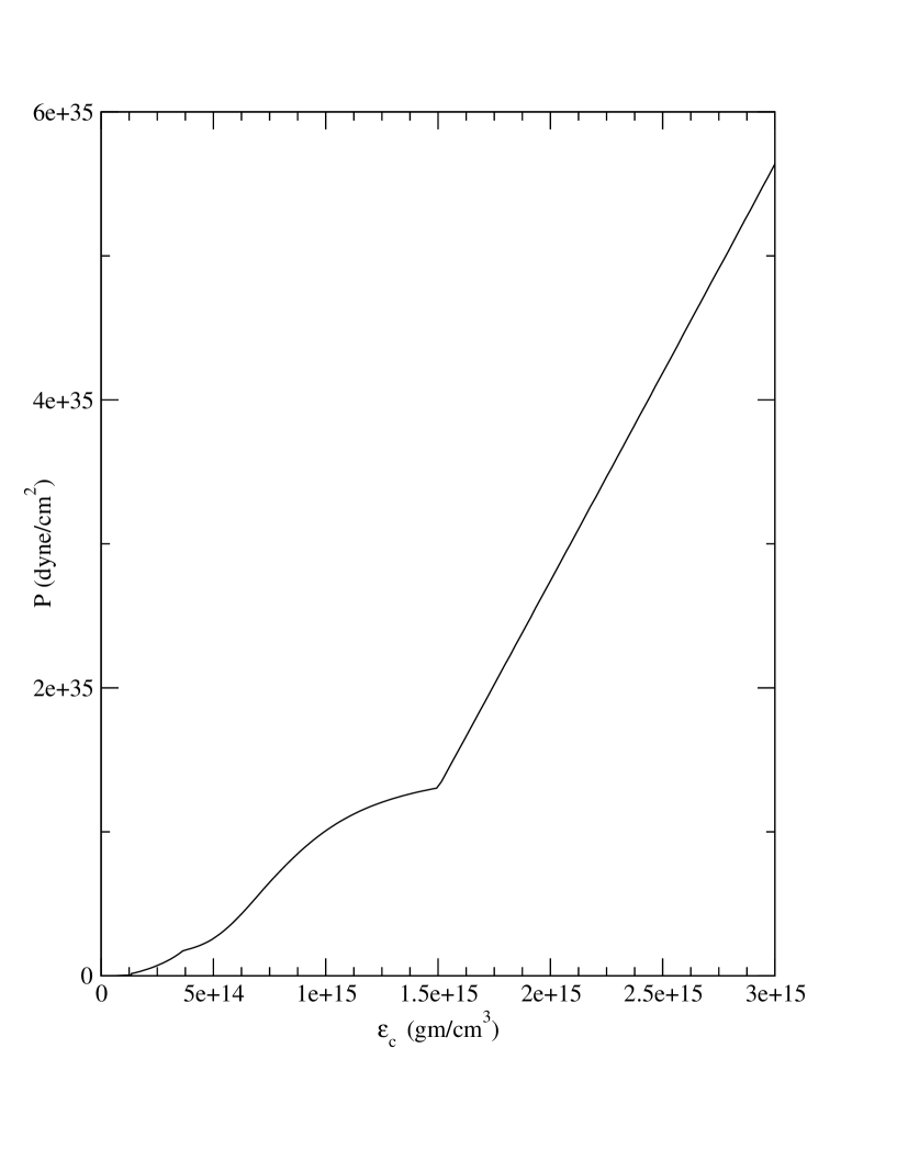
FIG. 1.: Equation of state of the model considered here.

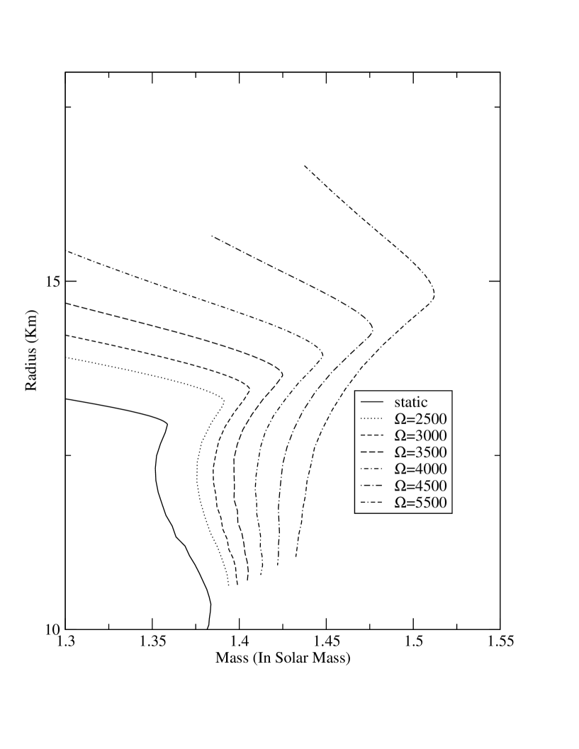
FIG. 2.: Radius-Mass plots for different $\Omega$.

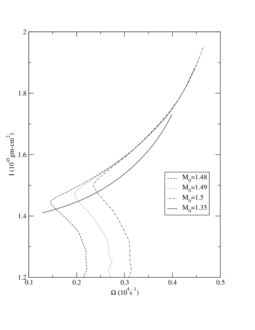
FIG. 3.: Moment of inertia as a function of $\Omega$ for different rest mass.

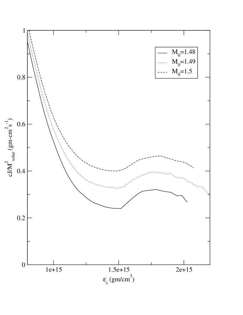
FIG. 4.: J as a function of $\epsilon_{c}$ for different rest mass.

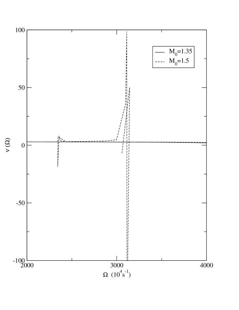
FIG. 5.: Braking index as a function of $\Omega$.

REFERENCES

- [1] F. Weber, ”Pulsars as Astrophysical Laboratories for Nuclear and Particle Physics” - Institute of Physics Publishing.
- [2] J. Alam, S. Raha and B. Sinha, Phys. Rep. 273, 243 (1996).
- [3] N. K. Glendenning, Phys. Rev. D46, 1274 (1992).
- [4] N. K. Glendenning, S. Pei and F. Weber, Phys. Rev. Lett. 79, 1603 (1997).
- [5] N. K. Spyrou and N. Stergioulas, Astron. & Astroph. 395, 151 (2002).
- [6] I. N. Mishustin, M. Hanauske, A. Bhattacharyya, L. M. Satarov, H. Stoecker and W. Greiner, Phys. Lett. B552, 1 (2003).
- [7] K. Schertler, C. Greiner, J. Schaffner-Bielich and M. Thoma, Nucl. Phy. A677, 463 (2000).
- [8] J. Schaffner and I. N. Mishustin, Phys.Rev. C43, 1416 (1996).
- [9] J. Boguta and A. R. Bodmer, Nucl. Phys. A292, 413 (1977); J. Boguta and H. Stöcker, Phys. Lett. B120, 289 (1983)
- [10] A. R. Bodmer, Nucl. Phys. A526, 703 (1991).
- [11] R. Brockmann, W. Weise, Phys. Lett. B69, 167 (1977); J. Boguta, S. Bohrmann, ibid. B102, 93 (1981); M. Rufa, H. Stöcker, P.-G. Reinhard, J. Maruhn, W. Greiner, J. Phys. G13, L143 (1987).
- [12] N. K. Glendenning and S. A. Moszkowski, Phys. Rev. Lett. 67, 2414 (1991).
- [13] J. Schaffner, C. Greiner, H. Stöcker, Phys. Rev. C46, 322 (1992).
- [14] C. B. Dover, D. J. Millener and A. Gal, Phys. Rep. 184, 1 (1989).
- [15] J. Schaffner, C. B. Dover, A. Gal, C. Greiner, H. Stöcker: Phys. Rev. Lett. 71, 1328 (1993).
- [16] J. Schaffner, C. B. Dover, A. Gal, C. Greiner and H. Stoecker; Ann. of Phys. (N.Y.) 235, 35 (1994).
- [17] A. Chodos, R. L. Jaffe, K. Johnson, C. B. Thorne and V. S. Weisskopf, Phys. Rev. D9, 3471 (1974).
- [18] H. Komatsu, Y. Eriguchi and I. Hachisu, Mon. Not. R. Astr. Soc. 237, 355 (1989).
- [19] G. B. Cook, S. L. Shapiro and S. A. Teukolsky, Ap. Jr. 424, 823 (1994).