Electron Abundance in Protostellar Cores

Abstract

The determination of the fractional electron abundance, $x_{\rm e}$, in protostellar cores relies on observations of molecules, such as DCO⁺, H¹³CO⁺ and CO, and on chemical models to interpret their abundance. Studies of protostellar cores have revealed significant variations of $x_{\rm e}$ from core to core within a range $10^{-8}<x_{\rm e}<10^{-6}$. The physical origin of these large variations in $x_{\rm e}$ is not well understood, unless unlikely variations in the cosmic ray ionization rate or ad hoc values of metal depletion are assumed. In this work we explore other potential causes of these variations in $x_{\rm e}$  including core age, extinction and density. We compute numerically the intensity of the radiation field within a density distribution generated by supersonic turbulence. Taking into account the lines of sight in all directions, the effective visual extinction in dense regions is found to be always much lower than the extinction derived from the column density along a fixed line of sight. Dense cores with volume and column densities comparable to observed protostellar cores have relatively low mass–averaged visual extinction, 2 mag $\leq A_{\rm V}\leq 5$ mag, such that photo–ionization can sometimes be as important as cosmic ray ionization. Chemical models, including gas–grain chemistry and time dependent gas depletion and desorption, are computed for values of visual extinction in the range 2 mag $\leq A_{\rm V}\leq 6$ mag, and for a hydrogen gas density of 10⁴ cm^-3, typical of protostellar cores. The models presented here can reproduce some of the observed variations of ion abundance from core to core as the combined effect of visual extinction and age variations. The range of electron abundances predicted by the models is relatively insenstive to density over 10⁴ to 10⁶ cm^-3.

1 Introduction

The fractional electron abundance, $x_{\rm e}=n_{\rm e}/n_{\rm H_{2}}$, is an important physical parameter in the chemistry of molecular gas because it controls the molecular ion abundance of the gas. The molecular ion abundance determines the coupling between the gas and the magnetic field and is therefore important for magneto–hydrodynamic (MHD) processes in molecular clouds. The ambipolar drift velocity of electrically neutral gas relative to charged particles (and magnetic field lines) can be expressed as $v_{\rm AD}\propto B^{2}/x_{\rm e}$, where $B$ is the magnetic field strength (assuming equilibrium of Lorentz and frictional forces).

The determination of $x_{\rm e}$ in protostellar cores relies on the observations of molecular ions, such as DCO⁺ and H¹³CO⁺ and on chemical models to interpret the abundance of such ions in relation to the value of $x_{\rm e}$. This method to determine $x_{\rm e}$ has been applied by Caselli et al. (1998) and Williams et al. (1998), using updated deuterium abundance and dissociative recombination rates of H${}_{3}^{+}$ and H₂D⁺, and complementary determinations of column density through observations of the transition J=1–0 of C¹⁸O. Observational results and predictions of the chemical models are compared on the $R_{\rm D}$–$R_{\rm H}$ plane, where $R_{\rm H}=$[HCO⁺]/[CO] and $R_{\rm D}=$[DCO⁺]/[HCO⁺] are molecular abundance ratios.

Significant variations from core to core in the value of $R_{\rm H}$ are found ($10^{-5}<R_{\rm H}<10^{-4}$), implying variations of $x_{\rm e}$ in the range $10^{-7.5}<x_{\rm e}<10^{-6.5}$, according to Williams et al. (1998), and $10^{-8}<x_{\rm e}<10^{-6}$ in the study by Caselli et al. (1998). The physical origin of these large variations of $x_{\rm e}$ is not well understood. The observed HCO⁺ abundances are matched by Caselli et al. (1998) by varying the cosmic ray ionization rate in the range $10^{-18}$ s${}^{-1}\leq\zeta_{\rm H_{2}}\leq 10^{-16}$ s^-1, and by Williams et al. (1998) by varying the metal depletion by a factor of 2–15 times their nominal values. However, the cosmic ray ionization rate has been measured to be $\zeta_{\rm H_{2}}=2.6\pm 1.8\times 10^{-17}$ s^-1 within massive protostellar envelopes, where photo–ionization is certainly insignificant (van der Tak & van Dishoeck 2000). Variations of two orders of magnitude in $\zeta_{\rm H_{2}}$ are not expected inside dense cores. Furthermore, there is no observational evidence for the specific values of metal depletion inferred by Williams et al. (1998); as those authors point out, gas–grain models (Bergin, Langer & Goldsmith 1995) predict a rather rapid metal depletion, and metal abundances significantly lower than assumed in their work are expected, decreasing as a function of age. This result is also confirmed by the models presented in this work (see § 5).

Here we investigate the possibility that the observed abundances of molecular ions and the inferred variations of $x_{\rm e}$ in protostellar cores are due to variations in age and extinction, $A_{\rm V}$, from core to core. In § 2 we show, based on numerical simulations, that dense cores formed by supersonic turbulent flows within molecular clouds can be much less opaque to UV photons than inferred from their observed column density, due to the very complex density distribution in the cloud and within the cores. In this work $\tau_{\rm v}$ is the effective visual extinction in three dimensional models, computed with the Monte Carlo radiative transfer code. $A_{\rm V}$ is the visual extinction through the line of sight, proportional to the column density in that direction. $A_{\rm V}$ is also used to refer to the visual extinction in the chemical models. Values of effective visual extinction, $\tau_{\rm v}$ , are found to be smaller than the extinction measured in the direction of a fixed line of sight.

In § 3 we present chemical models, including gas–grain chemistry and time dependent depletion and desorption. The models are computed for a range of core visual extinction including the values suggested by the radiative transfer models, 2 mag $\leq A_{\rm V}\leq 6$ mag, and for values of gas density typical of protostellar cores (and consistent with the density in the cores selected in the turbulence simulations), $n=10^{4}$ cm^-3. Models with $n=10^{5}$ cm^-3 and $n=10^{6}$ cm^-3 are also computed. We show in § 4 that the observed variations in ion abundances from core to core can be understood as the combined effect of variations in visual extinction and age (possibly gas density as well). Results are discussed in § 5, and conclusions are summarized in § 6.

2 UV Flux in Turbulent Clouds

The enhanced penetration of UV photons in clumpy or fractal molecular clouds has been discussed in previous works (Boissé 1990; Myers & Khersonsky 1995; Elmegreen 1997). Here we compute the radiation field within a density distribution that results from the numerical solution of the magneto–hydrodynamic (MHD) equations, in a regime of highly supersonic turbulence. The model we use is the final snapshot of the super–Alfvénic simulation presented in Padoan & Nordlund (1999). We refer the reader to that paper for a detailed description of the simulation. The numerical experiment is run on a 128³ staggered grid, with periodic boundary conditions, random external large scale forcing and an isothermal equation of state. Supersonic and super–Alfvénic turbulent flows have been shown to provide a good description of the dynamics of molecular clouds (e.g. Padoan & Nordlund 1999; Padoan et al. 1999, 2001).

The intensity of the radiation field is computed with a Monte Carlo method. Photon packages are sent into the cloud from the background and the scattering and absorption processes are simulated. The dust opacity is calculated from the relation between $N_{\rm H_{2}}$ and $A_{\rm V}$ as given by Bohlin, Savage & Drake (1978). The albedo of the grains is assumed to be 0.5 and the asymmetry factor of the scattering $g=0.6$ (e.g. Draine & Lee 1984).

The number of incoming photons is obtained for each cell at position ${\bf r}$, and the local value of the visual extinction, $\tau_{\rm v}({\bf r})$, is computed from the local intensity of the radiation field, $I({\bf r})$, relative to external radiation field, $I_{0}$:

$$\tau_{\rm v}({\bf r})=2.5\,{\rm log}_{10}({\rm e})\,\tau({\bf r})$$ (1)

where $\tau({\bf r})$ is the effective optical depth at the position ${\bf r}$,

$$\tau({\bf r})=-{\rm ln}\left[\frac{I({\bf r})}{I_{0}}\right]$$ (2)

and

$$I({\bf r})=\frac{1}{4\pi}\int{I({\bf r},\omega)\,d\omega}$$ (3)

where $I({\bf r},\omega)$ is the radiation field at the position ${\bf r}$ from the direction $\omega$.

Figure 1 shows volume projections of the density field (left panel) and visual extinction (right panel) in our model. Dense cores and filaments can be seen in the density field. The visual extinction increases gradually toward the center of the model and also inside the densest cores and filaments. Therefore, both the local density and the large scale structure affect the local value of the extinction.

The local value of $\tau_{\rm v}$ in the three dimensional model cannot be derived directly from the visual extinction through the line of sight, $A_{\rm V}$, corresponding to the column density along that line of sight. In Figure 2, left panel, the largest value of the local visual extinction, $\tau_{\rm v,max}$, along each of the lines of sight parallel to the three orthogonal axis of the numerical mesh, is plotted versus the visual extinction derived from the column density along that line of sight divided by two, $A_{\rm V,obs}$. The values of $\tau_{\rm v,max}$ are always much smaller than the values of $A_{\rm V,obs}$. The right panel of Figure 2 shows a linear–log plot of the histograms of the two quantities.

The result illustrated in Figure 2 implies that column density determinations cannot provide useful estimates of the actual $\tau_{\rm v}$ in dense regions of turbulent molecular clouds. More importantly, local values of $\tau_{\rm v}$ are likely to be a few times smaller than the observed $A_{\rm V,obs}$. This difference is due to the existence of directions with optical depth smaller than the specific line of sight of the observations and to the presence in the cloud of diffuse scattered radiation. This result should be taken into account when dust models are used to constrain dust temperature and emissivity in cores and when chemical models are used in combination with extinction measurements and chemical abundance determinations to constrain gas depletion.

We select dense cores in the MHD density snapshot as connected regions with gas density above 10⁴ cm^-3. This value is chosen to match the typical densities of protostellar cores and also for consistency with the observational sample in Williams et al. (1998), where cores are selected from their ammonia emission and have a typical density of approximately 10⁴ cm^-3. We compute the mass–averaged visual extinction in each core, $\langle\tau_{\rm v}\rangle$, assuming it is the appropriate value of visual extinction that should be used in single point chemical models to derive molecular abundances in the cores (the observed abundances are also approximately mass–averaged, given the low opacity of the observed transitions of DCO⁺, H¹³CO⁺ and C¹⁸O). The mass–averaged visual extinction also has the advantage of being only weakly dependent on the density threshold used to select the cores.

We compute the total mass and volume of each core, and use them to derive the core column density assuming a spherical shape, as an estimate of the average core column density. The visual extinction to the center of each core corresponding to this value of column density is called $A_{\rm V,0}$. As illustrated in Figure 3 (left panel), values of $\langle\tau_{\rm v}\rangle$ in dense cores are always significantly lower than the extinction derived from half the value of their column density, $A_{\rm V,0}$. The difference between values of $\langle\tau_{\rm v}\rangle$ in cores and the extinction derived from half the value of the column density at the line of sight through the core center, $A_{\rm V,obs}$, is even greater, as shown in the right panel of Figure 3. This can be explained as due to the elongated shape of cores in numerical simulations, consistent with typical aspect ratios in observed cores (Myers et al. 1991), and to density structures along the line of sight to a core and within the core (lines of sight perpendicular to the elongated structure have more weight in determining the value of $\tau_{\rm V}$).

Observed column densities almost always overestimate the core’s true opacity to UV photons (especially at the largest values of $A_{\rm V,obs}$), since these always penetrate preferentially along directions of lowest column density (for example the core shortest axis). The local extinction, $\tau_{\rm v}({\bf r})$, is significantly smaller than the extinction corresponding to the average optical depth, $\langle\tau({\bf r},\omega)\rangle_{\omega}$. This result can be easily understood in the absence of scattering or if the scattering is only forward. The local radiation field from the direction $\omega$ can then be expressed as a function of the local optical depth from that direction, $I({\bf r},\omega)=I_{0}\,{\rm exp}[-\tau({\bf r},\omega)]$, and the local extinction is given by an average of ${\rm exp}[-\tau({\bf r},\omega)]$ The directions of lowest optical depth have therefore a dominant contribution to the average extinction.

Squares in Figure 3 represent cores at the distance from the cloud center smaller than $\langle R\rangle$, while asterisks represent cores at a distance from the cloud center larger than $\langle R\rangle$, where $\langle R\rangle$ is the average of the distances of all selected cores to the cloud center (the center of the computational mesh). The figure shows that the visual extinction increases towards the cloud center. Furthermore, the left panel shows that the extinction also increases with the cores mass. This shows again the visual extinction is determined both by the local mass distribution in an individual core and by the cloud structure on a larger scale.

The cores we have selected from the MHD simulation have volume and column densities typical of observed protostellar cores. In the core sample by Williams et al. (1998), the column densities estimated by the intensity of the J=1–0 line of C¹⁸O correspond to $A_{\rm V,obs}$ in the range $\sim$5–20 mag (the total extinction along the line of sight divided by two), as in our numerical sample (see Figure 3, right panel). Since in our numerical sample we find corresponding values of $\langle\tau_{\rm v}\rangle$ in the range $\sim$2–5 mag (Figure 3), we can infer that the dense cores in the sample by Williams et al. (1998) may also have similarly low values of mass–averaged visual extinction, $\langle\tau_{\rm v}\rangle$.

The photoionization rate is larger than the cosmic ray ionization rate at $A_{\rm V}<4$ mag (McKee 1989). Equilibrium abundances of molecules and fractional ionization are sensitive to the value of $A_{\rm V}$ also for $A_{\rm V}\leq 4$ mag. Based on the low values of $\langle\tau_{\rm v}\rangle$ predicted in this work, photoprocesses in protostellar cores could therefore be more important than assumed in previous studies.

3 Chemical Models of Cloud Cores

The chemical model is based on Willacy & Millar (1998) and includes deuterium reactions. Gas phase molecules freezeout onto dust grains at a rate of

$$\frac{dn_{\rm x}}{dt}=Cs_{\rm x}\langle\pi\,a^{2}n_{\rm g}\rangle\,v_{\rm x}n_{\rm x}\,\,\,{\rm cm}^{-3}{\rm s}^{-1}$$ (4)

where $s_{\rm x}$ is the sticking coefficient ($s_{\rm x}=0.3$ for all species), $a$ is the grain radius, $n_{\rm g}$ is the number density of grains (equal to $10^{-12}n_{H}$), $v_{\rm x}$ is the thermal velocity, and $n_{\rm x}$ is the number density of the species x. $C$ is a factor that accounts for the expected increase of the freezeout rate of positive ions onto negative grains. For neutrals $C=1$, while for ions $C=1+16.71\times 10^{-4}/(a\,T)$ (Rawlings et al. 1992).

We assume that H⁺, H${}_{2}^{+}$, H${}_{3}^{+}$, their deuterated equivalents and He⁺ are neutralized on collision with grains and returned to the gas. Desorption due to cosmic ray induced heating of grains is also included, using the rates given in Hasegawa & Herbst (1993). The time evolution of the abundance of some molecular species is plotted in Figure 4. The elemental abundances are given in Table 1 relative to $n(\rm H_{tot})$, where $n(\rm H_{tot})=2n({\rm H}_{2})+n({\rm H})$.

The main parameters of chemical models are the visual extinction, $A_{\rm V}$, the gas temperature, $T$, the gas density $n$, the cosmic ray ionization rate for molecular hydrogen, $\zeta_{\rm H_{2}}$, the initial abundances of atomic species and the factor $\chi$ by which the interstellar radiation field is enhanced relative to its standard value of $1.6\times 10^{-3}$ ergs cm^-2 s^-1 (Habing 1968). In this work, we assume a temperature of $T=10$ K for both the gas and the dust, a cosmic ray ionization rate of $\zeta_{\rm H_{2}}=1.2\times 10^{-17}$ s^-1 and a standard value of the interstellar radiation field ($\chi=1.0$).

Single point models are run for three values of molecular hydrogen gas density, $n=10^{4}$, $10^{5}$ and $10^{6}$ cm^-3, and for nine values of extinction ($A_{\rm V}=2.0$, 2.5, 3.0, 3.5, 4.0, 4.5, 5.0, 5.5 and 6.0 mag) at each density. As discussed above, the values of visual extinction are taken from the MHD models, which are consistent with the column densities of the observational sample in Williams et al. (1998). To simulate the evolution of gas under diffuse conditions before it is incorporated into a core, we used the steady-state output of a gas phase only model with density = 10³ cm^-3 and $A_{v}$ = 3 to provide the input abundances for the models presented here. The input elemental abundances for the gas phase model are given in Table 1.

4 Results

In this section, results from the chemical models are compared with observational data with the aim of determining whether variations in the model parameters such as $A_{\rm V}$, time and density can account for the observed scatter in [DCO⁺]/[HCO⁺] and [HCO⁺]/[CO] . The observational [DCO⁺]/[HCO⁺] and [HCO⁺]/[CO] values are obtained by selecting only the starless cores from the samples in Williams et al. (1998) and Butner, Lada and Loren (1995). NH₃ and N₂H⁺ abundances for a subsample of those starless cores are taken respectively from Jijina, Myers and Adams (1999) and from Caselli et al. (2002a). The densities of the cores in the sample of Williams et al. (1998) lie in the approximate range of a few x 10³ to 10⁵ cm^-3. Here we adopt a model density of 10⁴ cm^-3 as our baseline for comparison with the observations. Changes in model density cause some variation in the results, but by far the largest effects are caused by variations in $A_{\rm V}$ or time.

The time-dependent abundances of some important species are shown in Figure 4 for a model with $n=10^{4}$ cm^-3 and $A_{\rm V}$= 5.5 mag. The abundance of CI drops off due to accretion and to gas phase conversion into CO, but rises again slightly after a few $\times$ 10⁵ years, where the desorption of CH₄ due to cosmic ray heating provides a means by which a low level of carbon atoms can be maintained in the gas. (The CH₄ is produced by hydrogenation of CI on grain surfaces). As expected the abundance of HCO⁺ and DCO⁺ follows that of CO and N₂H⁺ begins to deplete at later times than CO.

The main problem in estimating the electron abundance in protostellar cores is the difficulty of observing directly some of the most abundant molecular ions, such as H${}_{3}^{+}$ and H₃O⁺, and atomic carbon and metals with low ionization potential. Values of $x_{\rm e}$ are therefore determined by matching the observed abundances of other molecular ions such as HCO⁺ and DCO⁺, with chemical models. These molecular ions are predicted to be the main carriers of charge at the relevant core timescales. The comparison between observed and predicted abundances is greatly affected by the depletion of gas species on dust grains. Evidence of CO depletion has been provided for many dense protostellar cores (Willacy et al. 1998; Caselli et al. 1999; Tafalla et al. 2002; Jessop & Ward-Thompson 2001; Bergin et al. 2002; Hotzel et al. 2002; Bacmann et al. 2002; Caselli et al. 2002b; Juvela et al. 2002). The depletion rate is directly proportional to the gas density and models have shown that some molecules such as CO are removed from the gas more quickly than others e.g. N₂H⁺, NH₃ because of chemical effects (see Figure 4). As a result cores are expected to show chemical differentiation with species such as HCO⁺ and DCO⁺ being preferentially located in the outer layers of cores where the density may be lower or the chemistry is less evolved, and the denser, more evolved inner regions of the cores being better traced by N₂H⁺ and N₂D⁺ (Kuiper et al. 1996, Caselli et al. 2002b). Spatial variations of abundances due to depletion are a source of uncertainty in the comparison of single point chemical models with the observations, even if the time evolution of the depletion is modeled as in this work. However the combination of a variety of tracers can give clues as to the chemical age of the cores.

Figure 5 shows the variation in abundance ratios of several molecules with $A_{\rm V}$ for $n$ = 10⁴ cm^-3. Three model times are shown: 4 $\times$ 10⁴, 10⁵ and 3 $\times$ 10⁵ years. We find that the abundances at later times are not consistent with the observed values and that the cores appear to be chemically young. However for a fixed density and $A_{v}$ no single model can explain all of the observations. One possibility is that the emission from different molecules may originate from different regions of the cloud as discussed above (c.f. Kuiper et al. 1996, Caselli et al. 2002b).

Figure 6 shows the results for the model with n = 10⁴ cm^-3 plotted on the $R_{\rm D}$–$R_{\rm H}$ plane, where $R_{\rm D}$=[DCO⁺]/[HCO⁺], and $R_{\rm H}$=[HCO⁺]/[CO]. Squares show the $R_{\rm D}$–$R_{\rm H}$ values of the observed starless cores. The solid lines show the variations in abundance for different values of $A_{\rm V}$ for fixed ages of $4\times 10^{4}$ yr, $10^{5}$ yr and $3\times 10^{5}$ yr, with the bottom of the curves corresponding to $A_{\rm V}$= 3 mag and the top to $A_{\rm V}$= 6 mag. The filled diamonds correspond to $A_{\rm V}$=3.5 mag. The free–fall time at this density is $t_{\rm ff}=3.5\times 10^{5}$ yr. Figure 6 shows that variations in age and extinction can explain some, but not all, of the observed scatter in the $R_{\rm D}$–$R_{\rm H}$ plane, at a fixed density of $n=10^{4}$ cm^-3. Increasing the density moves the curves down slightly but not sufficiently to account for the three cores in the bottom right hand corner of the $R_{\rm D}$–$R_{\rm H}$ plane.

Figure 7 shows time evolution tracks of models with $n=10^{4}$ cm^-3 and $A_{\rm V}$=3 mag, $A_{\rm V}$=3.5 mag and $A_{\rm V}$=6 mag on the $R_{\rm D}$–$R_{\rm H}$ plane. Each track is shown as a solid line for an age up to $10^{5}$ yr, as a dashed line between $10^{5}$ yr and $2\times 10^{5}$ yr, and as a dotted line between $2\times 10^{5}$ yr and $10^{6}$ yr. Solid diamonds correspond to $t=t_{\rm ff}=3.5\times 10^{5}$ yr. As suggested by the isochrones, some of the scatter in the observational $R_{\rm D}$–$R_{\rm H}$ plane can be explained by reasonable variations of age and visual extinction from core to core. However, considering the observational error bars, five cores cannot be fit by our models: three of these have high [DCO⁺]/[HCO⁺] and low [HCO⁺]/[CO] , one low [DCO⁺]/[HCO⁺] and high [HCO⁺]/[CO] and one both low [DCO⁺]/[HCO⁺] and low [HCO⁺]/[CO] . We find that rather young cores fit the observations, with ages smaller than $t_{\rm ff}$.

Figure 7 also shows that, for fixed values of extinction, $A_{\rm V}$$\geq 3.5$ mag, and density, $n=10^{4}$ cm^-3, cores can span some of the range of observed [DCO⁺]/[HCO⁺] and [HCO⁺]/[CO] values for timescales of less than 0.2 Myr. Observed values of [DCO⁺]/[HCO⁺] have been recently used to estimate the “chemical age” of cloud cores in Taurus (Saito et al. 2002).

The same time evolution tracks from Figure 7 are plotted in Figure 8 on the planes [DCO⁺]/[HCO⁺]–$x_{\rm e}$ (top panel) and [HCO⁺]/[CO]–$x_{\rm e}$ (bottom panel). The electron abundance decreases with time, reaching a minimum at an age of approximately 0.2 Myr for the model with $A_{\rm V}$=6 mag. As can be seen in Figure 9, the electron abundance is anticorrelated with the abundance of molecular ions such as HCO⁺, H₃O⁺ and H${}_{3}^{+}$, as these ions are responsible for most recombinations. These molecular ions are also the main charge carriers for core ages greater than 0.1 Myr, while for younger cores the metals are the main charge carriers (Figure 9). Metal ions are initially more abundant than molecular ions because molecules are still being formed, and freezeout has not yet removed the metals from the gas.

Williams et al. (1998) estimated values of electron abundance in the range $3\times 10^{-8}<x_{\rm e}<2\times 10^{-7}$ for the cores in their sample, excluding B133. Our models give smaller values and a smaller range of electron abundances, $1.5\times 10^{-8}<x_{\rm e}<7\times 10^{-8}$.

The models of Williams et al. consider a gas phase only chemistry with the effects of freezeout being modeled by considering variations in the atomic carbon, oxygen and metal abundances. In contrast, our model includes explicit consideration of the time-dependent depletion of the molecules from the gas. The values of depletion we estimate for the observed cores are much larger than in Williams et al. (1998). The abundance of Si⁺ can be used for a comparison. Williams et al. (1998) find solutions for most of the cores in their sample with Si⁺ abundance values in the range $2.7\times 10^{-9}<\rm{[Si^{+}]/[H_{2}]}<2.0\times 10^{-8}$. The highest depletion, $\rm{[Si^{+}]/[H_{2}]}=2.7\times 10^{-9}$, corresponds to the lowest electron abundance and the highest [HCO⁺]/[CO] value. In the models used in this work the depletion of metals increases with time. The initial Si⁺ abundance is $\rm{[Si^{+}]/[H_{2}]}=4\times 10^{-8}$. At the free–fall time ($3.5\times 10^{5}$ yr for $n=10^{4}$ cm^-3), $\rm{[Si^{+}]/[H_{2}]}=5.0\times 10^{-10}$ in the model with $A_{\rm V}$=6 mag and $\rm{[Si^{+}]/[H_{2}]}=4.4\times 10^{-10}$ in the model with $A_{\rm V}$=3 mag. At an age of $t=1$ Myr the abundances for the same two models are $\rm{[Si^{+}]/[H_{2}]}=3.4\times 10^{-12}$ and $\rm{[Si^{+}]/[H_{2}]}=6.6\times 10^{-14}$ respectively. Metal depletion is therefore important even for core ages as low as one free–fall time.

According to the models used in this work, metal depletion is 10 to 10⁵ times larger than assumed in Williams et al. (1998), even with cosmic ray desorption. One of the reasons for the Williams et al. approach in using only gas phase chemistry was that they found that the vertical spread of their results in the $R_{\rm D}$–$R_{\rm H}$ plane disappeared with the inclusion of a gas-grain chemistry, as a result of the rapid accretion of metal ions. In our models some vertical spread can be obtained due to both differences in time and in $A_{\rm V}$, but density has little effect. Although we are not able to reproduce as large a vertical spread as Williams et al.  the present models are still able to produce some of the observed scatter in [DCO⁺]/[HCO⁺] and [HCO⁺]/[CO].

On the other hand, CO depletion is not very strong for ages up to 1 Myr, as shown in Figure 4. The CO abundance varies by less than a factor of two between $t=0.1$ Myr and $t=0.5$ Myr. The uncertainty in the core C¹⁸O column density values due to variations of the C¹⁸O abundance should be less than a factor of two, which does not affect significantly the results of this work.

Assuming that the electron abundance, $x_{\rm e}$, is determined by cosmic ray ionization balanced by recombination, $x_{\rm e}$ can be expressed as

$$x_{\rm e}=C_{\rm i}\,n^{-1/2}\,\zeta_{\rm H_{\rm 2}}^{1/2}$$ (5)

where $C_{\rm i}$ is a constant that depends on the relative contributions of molecular ions and metals to the ionization balance. This expression for $x_{\rm e}$ would be appropriate for cores where $A_{\rm V}$ $>$ 4, where ionization due to cosmic rays dominates that resulting from UV radiation. McKee (1989) derives $C_{\rm i}=3.2\times 10^{3}$ cm^-3/2s^1/2 (dotted line in Figure 9), while Williams et al. (1998) obtained $C_{\rm i}=2.0\times 10^{3}$ cm^-3/2s^1/2. Both these values of $C_{i}$ produce $x_{\rm e}$ that is a factor of 3 – 5 higher than predicted by the current models for $n=10^{4}$ cm^-3 and $A_{\rm V}$ = 6 (Figure 9). Figure 9 also shows that $x_{\rm e}$ varies with time by approximately a factor of 2. Also if $A_{\rm V}$ is less than 4 mag, then the UV field will be important in determining the value of $x_{\rm e}$  and since variations in $A_{\rm V}$ can account for some of the spread in $R_{\rm D}$–$R_{\rm H}$ a more complete consideration of the chemistry is required to determine $x_{\rm e}$.

5 Conclusions

This work presents a partial solution to the problem of the large scatter in the observed values of [DCO⁺]/[HCO⁺] and [HCO⁺]/[CO] in protostellar cores. It is shown that variations in [DCO⁺]/[HCO⁺] and [HCO⁺]/[CO] from core to core can be interpreted as the result of age and visual extinction variations. However, it is unable to explain all of the variations, in particular those cores with high [DCO⁺]/[HCO⁺] and low [HCO⁺]/[CO] and the one core with low [DCO⁺]/[HCO⁺]Ṫhis interpretation also implies the following conclusions:

• The electron abundance in the observed protostellar cores is in the range $1.5\times 10^{-8}<x_{\rm e}<7\times 10^{-8}$.

• Protostellar cores in this sample are relatively young, with ages from a fraction of a free–fall time to one free–fall time.

• A range of effective extinction between 2.5 and 5–6 mag is required by the observations (the upper limit is not well defined since the chemical models are not very sensitive to extinction for $A_{\rm V}$$>5$ mag), consistent with the mass–averaged extinction of dense cores in simulations of supersonic MHD turbulence.

This solution to the problem of the large scatter in the observed values of [DCO⁺]/[HCO⁺] and [HCO⁺]/[CO] in protostellar cores appears to be more consistent with the observational data than the alternative solutions proposed by Caselli et al. (1998) and Williams et al. (1998). Caselli et al. (1998) used a very large range of values for the cosmic ray ionization rate, which is not supported by observations of dense cores. Williams et al. (1998) used a very small value of metal depletion, which is not expected to hold for dense cores, even in the presence of desorption mechanisms. On the contrary, the present work is based on models with a realistic value of the cosmic ray ionization rate and a self–consistently determined value of metal depletion.

Figure captions:

Figure 1: Left panel: Volume projection of the density field from the MHD simulation used in this work. Dark is large density. Right panel: Volume projection of the effective visual extinction, $\tau_{\rm v}$, assuming an isotropic radiation field outside of the computational mesh, within the same mass distribution shown in the left panel. Dark is large visual extinction.

Figure 2: Left panel: Scatter plot of the maximum extinction within a line of sight, $\tau_{\rm v,max}$, versus the extinction due to half of the total column density of that line of sight, $A_{\rm V,obs}$. Right panel: Lin–log plot of the histograms of the two quantities plotted in the left panel.

Figure 3: Left panel: Mass averaged visual extinction, $\langle\tau_{\rm v}\rangle$, within the model cores selected from the MHD simulation, versus their extinction derived from their mass assuming spherical uniform density distribution, $A_{\rm V,0}$. The respective core mass values range from approximately 1 to 200 solar masses. $\langle R\rangle$ is the average distance of cores to the cloud center. Cores near the cloud center ($R<\langle R\rangle$) have larger visual extinction than cores closer to the cloud surface ($R>\langle R\rangle$). Right panel: Mass–averaged visual extinction, $\langle\tau_{\rm v}\rangle$, within the model cores selected from the MHD simulation, versus the extinction due to half of the total column density along the line of sight through the same cores, $A_{\rm V,obs}$. The model cores have values of $A_{\rm V,obs}$ comparable to the ones found in the protostellar core sample by Williams et al. (1998), but their mass–averaged effective extinction, $\langle\tau_{\rm v}\rangle$, is significantly smaller.

Figure 4: Time evolution of molecular abundances in the model with $n=10^{4}$ cm^-3 and $A_{\rm V}$=5.5 mag. The abundances of HCO⁺, N₂H⁺ and DCO⁺ have been multiplied by a factor of 1000. The dashed line labeled ’Metals⁺’ gives the sum of the abundances of C⁺, Si⁺, Fe⁺, N⁺ and O⁺.

Figure 5: Isochrones of models with $n=10^{4}$ cm^-3. Each curve represents the variation in abundances for different values of $A_{\rm V}$(ranging from $A_{\rm V}$= 3 mag at the bottom of the curve to $A_{\rm V}$= 6 mag at the top) at a fixed time $4\times 10^{4}$ yr, $10^{5}$ yr and $3\times 10^{5}$ yr (solid lines). Squares correspond to a subsample of the starless cores from Butner, Lada and Loren (1995) and Williams et al. (1998) for which NH₃ and N₂H⁺ abundances were given by Jijina, Myers and Adams (1999) and by Caselli et al. (2002a). Filled diamonds correspond to $A_{\rm V}$= 3.5 mag. a) [NH₃]/[CO] versus [DCO⁺]/[HCO⁺]; b) [N₂H⁺]/[CO] versus [DCO⁺]/[HCO⁺]; c) [N₂H⁺]/[NH₃] versus [DCO⁺]/[HCO⁺]; d) [N₂H⁺]/[CO] versus [HCO⁺]/[CO].

Figure 6: Isochrones of models with $n=10^{4}$ cm^-3. Each curve represents the variation in abundances for different values of $A_{\rm V}$(ranging from $A_{\rm V}$= 3 mag at the bottom of the curve to $A_{\rm V}$= 6 mag at the top) at a fixed time $4\times 10^{4}$ yr, $10^{5}$ yr and $3\times 10^{5}$ yr (solid lines). Squares correspond to the starless cores from the samples in Butner, Lada and Loren (1995) and Williams et al. (1998). Filled diamonds correspond to $A_{\rm V}$= 3.5 mag.

Figure 7: Time evolution tracks of models with $n=10^{4}$ cm^-3, for $A_{\rm V}$=3 mag, $A_{\rm V}$=3.5 mag and $A_{\rm V}$=6 mag on the $R_{\rm D}$–$R_{\rm H}$ plane. Each track is shown as a solid line for an age up to $10^{5}$ yr, as a dashed line between $10^{5}$ yr and $2\times 10^{5}$ yr, and as a dotted line between $2\times 10^{5}$ yr and $10^{6}$ yr. Filled circles correspond to the free–fall time, $t=t_{\rm ff}=3.5\times 10^{5}$ yr. Squares correspond to the starless cores from the samples in Butner, Lada and Loren (1995) and Williams et al. (1998).

Figure 8: Tracks showing the time evolution of the electron abundance, $x_{\rm e}$for models with $n=10^{4}$ cm${}^{-}3$ and $A_{\rm V}$=3, 3.5 and 6 mag on the $R_{\rm D}$–$R_{\rm H}$ plane. Each track is shown as a solid line for an age up to 10⁵ yr, as a dashed line between 10⁵ and 2 $times$ 10⁵ yr, and as a dotted line between 2 $\times$ 10⁵ yr and 10⁶ yr.

Figure 9: Ion and electron abundances versus time in the model with $n=10^{4}$ cm^-3 and $A_{\rm V}$=5.5 mag. The electron abundance according to the results of Williams et al. (1998) ($x_{\rm e}$= $C_{i}n^{-1/2}\zeta_{\hbox{H}_{2}}^{1/2}$ where $C_{i}$ = 2.0 $\times$ 10³ cm^-3/2s^1/2) is shown for comparison.

X	$n({\rm X})/n({\rm H}_{\rm tot})$
H2	0.495
HD	1.6e-5
N	2.14e-5
O	1.76e-4
Si	2.0e-8
C+	7.3e-5
Fe+	1.0e-8
CO	0
HCO+	0
DCO+	0

Table 1: Initial chemical abundances relative to $n(\rm H_{tot})$, where $n(\rm H_{tot})=2n({\rm H}_{2})+n({\rm H})$.

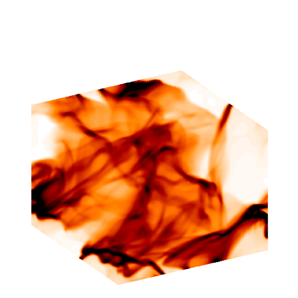
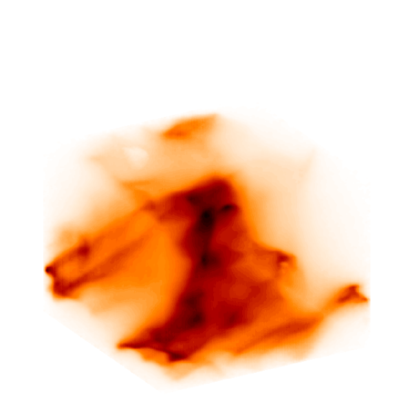
Figure 1:

Figure 2:

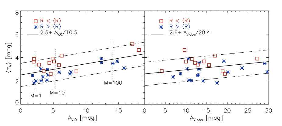
Figure 3:

Figure 4:

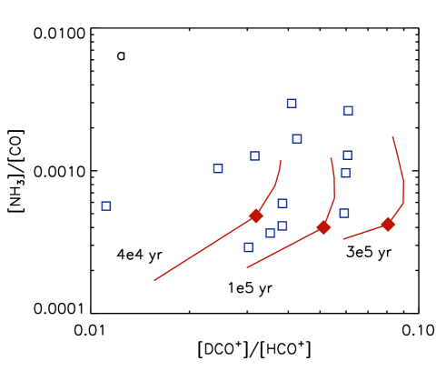
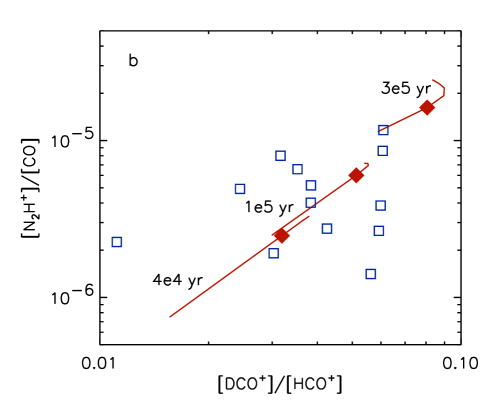
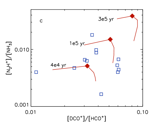
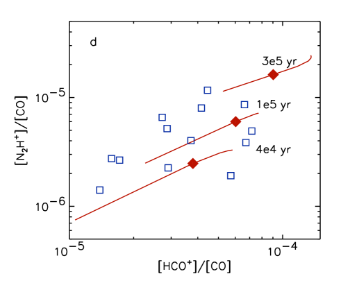
Figure 5:

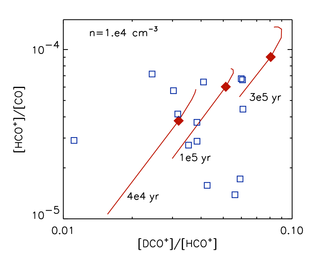
Figure 6:

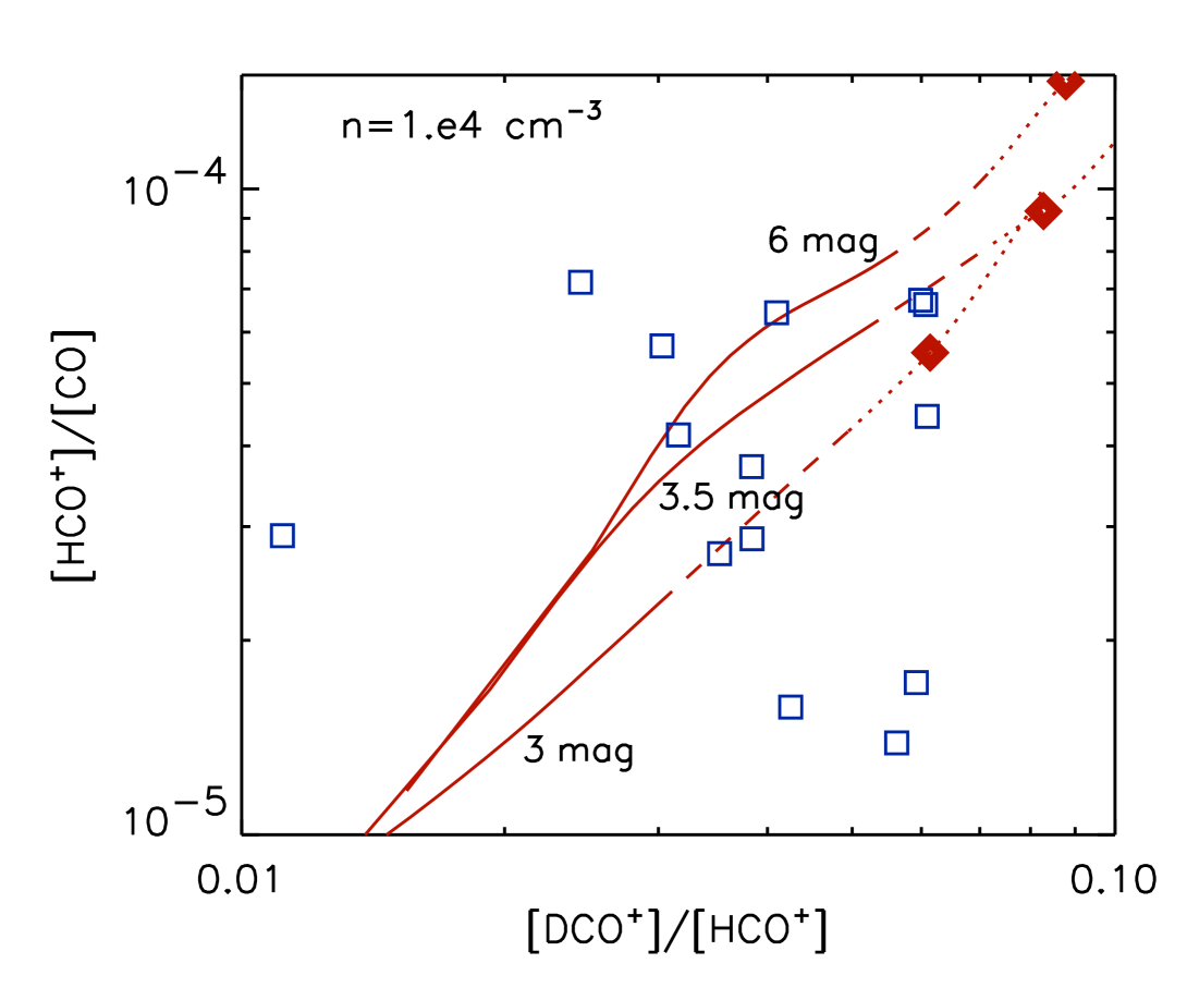
Figure 7:

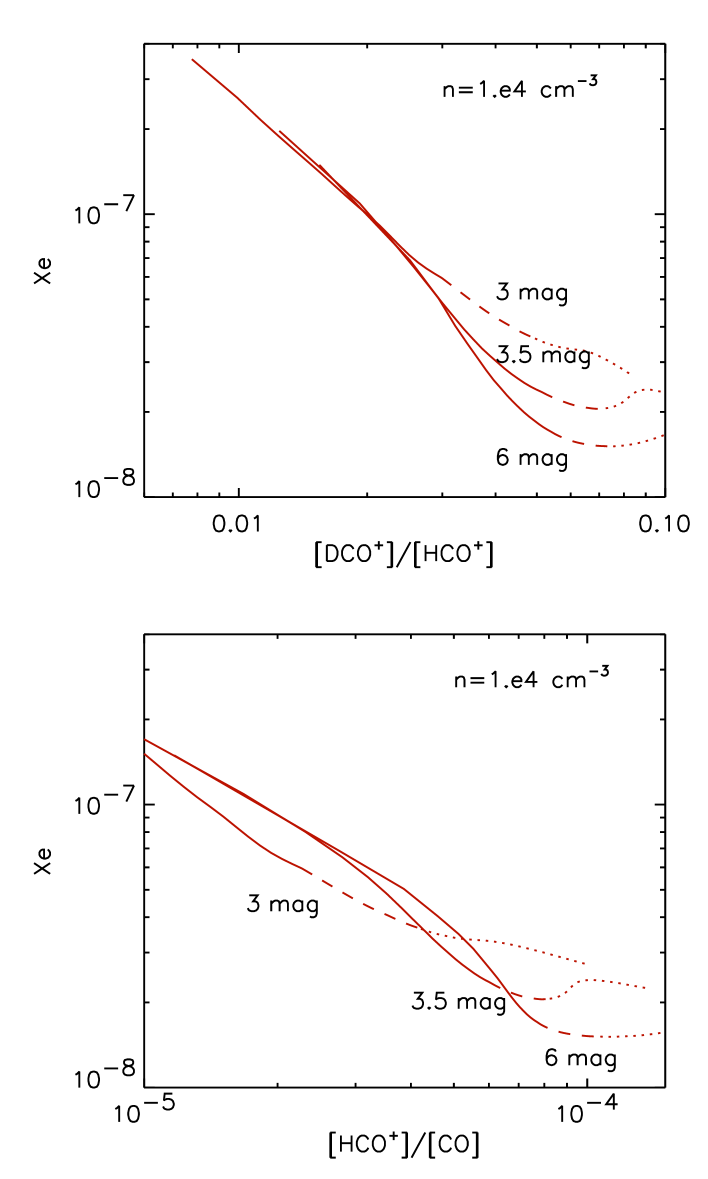
Figure 8:

Figure 9:

References

- Bacmann et al. (2002) Bacmann, A., Lefloch, B., Ceccarelli, C., Castets, A., Steinacker, J., & Loinard, L. 2002, A&A, 389, L6
- Bergin et al. (2002) Bergin, E. A., Alves, J., Huard, T., & Lada, C. J. 2002, ApJL, 570, L101
- Bergin et al. (1995) Bergin, E. A., Langer, W. D., & Goldsmith, P. F. 1995, ApJ, 441, 222
- Bohlin et al. (1978) Bohlin, R. C., Savage, B. D., & Drake, J. F. 1978, ApJ, 224, 132
- Boissé (1990) Boissé, P. 1990, A&A, 228, 483
- Butner et al. (1995) Butner, H. M., Lada, E. A., & Loren, R. B. 1995, ApJ, 448, 207
- Caselli et al. (2002a) Caselli, P., Benson, P. J., Myers, P. C., & Tafalla, M. 2002a, ApJ, 572, 238
- Caselli et al. (1999) Caselli, P., Walmsley, C. M., Tafalla, M., Dore, L., & Myers, P. C. 1999, ApJL, 523, L165
- Caselli et al. (1998) Caselli, P., Walmsley, C. M., Terzieva, R., & Herbst, E. 1998, ApJ, 499, 234
- Caselli et al. (2002b) Caselli, P., Walmsley, C. M., Zucconi, A., Tafalla, M., Dore, L., & Myers, P. C. 2002b, ApJ, 565, 344
- Draine & Lee (1984) Draine, B. T. & Lee, H. M. 1984, ApJ, 285, 89
- Elmegreen (1997) Elmegreen, B. G. 1997, ApJ, 477, 196
- Habing (1968) Habing, H. J. 1968, BAIN, 19, 421
- Hasegawa & Herbst (1993) Hasegawa, T. I. & Herbst, E. 1993, MNRAS, 261, 83
- Hotzel et al. (2002) Hotzel, S., Harju, J., Juvela, M., Mattila, K., & Haikala, L. K. 2002, A&A, 391, 275
- Jessop & Ward-Thompson (2001) Jessop, N. E. & Ward-Thompson, D. 2001, MNRAS, 323, 1025
- Jijina et al. (1999) Jijina, J., Myers, P. C., & Adams, F. C. 1999, ApJS, 125, 161
- Juvela et al. (2002) Juvela, M., Mattila, K., Lehtinen, K., Lemke, D., Laureijs, R., & Prusti, T. 2002, A& A, 382, 583
- Kuiper et al. (1996) Kuiper, T. B. H., Langer, W. D. & Velusamy, T. 1996, ApJ, 468, 761
- McKee (1989) McKee, C. F. 1989, ApJ, 345, 782
- Myers et al. (1991) Myers, P. C., Fuller, G. A., Goodman, A. A., & Benson, P. J. 1991, APJ, 376, 561
- Myers & Khersonsky (1995) Myers, P. C. & Khersonsky, V. H. 1995, ApJ, 442, 186
- Padoan et al. (1999) Padoan, P., Bally, J., Billawala, Y., Juvela, M., & Nordlund, Å. 1999, ApJ, 525, 318
- Padoan et al. (2001) Padoan, P., Juvela, M., Goodman, A. A., & Nordlund, Å. 2001, ApJ, 553, 227
- Padoan & Nordlund (1999) Padoan, P. & Nordlund, Å. 1999, ApJ, 526, 279
- Rawlings et al. (1992) Rawlings, J. M. C., Hartquist, T. W., Menten, K. M., & Williams, D. A. 1992, MNRAS, 255, 471
- Roberts & Millar (2000) Roberts, H. & Millar, T. J. 2000, A&A, 361, 388
- Saito et al. (2002) Saito, S., Aikawa, Y., Herbst, E., Ohishi, M., Hirota, T., Yamamoto, S., & Kaifu, N. 2002, ApJ, 569, 836
- Tafalla et al. (2002) Tafalla, M., Myers, P. C., Caselli, P., Walmsley, C. M., & Comito, C. 2002, ApJ, 569, 815
- van der Tak & van Dishoeck (2000) van der Tak, F. F. S. & van Dishoeck, E. F. 2000, A&A, 358, L79
- Willacy et al. (2002) Willacy, K., Langer, W. D., & Allen, M. 2002, ApJL, 573, L119
- Willacy et al. (1998) Willacy, K., Langer, W. D., & Velusamy, T. 1998, ApJL, 507, L171
- Willacy & Millar (1998) Willacy, K. & Millar, T. J. 1998, MNRAS, 298, 562
- Williams et al. (1998) Williams, J. P., Bergin, E. A., Caselli, P., Myers, P. C., & Plume, R. 1998, ApJ, 503, 689
- Xie et al. (1995) Xie, T., Allen, M., & Langer, W. D. 1995, ApJ, 440, 674