We study the cosmological dynamics of an effective theory for a strongly coupled scalar field in the moduli space of $\mathcal{N}=4$ supersymmetric Yang-Mills theory recently proposed by Silverstein and Tong, called ”D-cceleration”. We discuss various Energy Conditions in this theory. Then we prove the inflationary attractor property using the Hamilton-Jacobi method and study the phase portrait as well as the cosmological evolution of the scalar field.

Cosmological dynamics of D-cceleration

I Introduction

It is a great challenge to implement inflation in string/M-theory. Currently, to achieve this goal, there are mainly two types of models: one is the modification of the Friedmann equation in the braneworld scenario (see, e.g. brane for a review); another is specific model of inflaton field from string/M-theory (see, Linde for a recent important development). In this paper, we will consider a scenario belonging to the second type recently proposed by Silverstein and Tong Tong .

In Tong , Silverstein and Tong considered the inflaton as the scalar field in the moduli space of the $\mathcal{N}=4$ supersymmetric Yang-Mills (SYM) theory. They call this model ”D-cceleration”. In the strong coupling region, the effective description of the theory is via gravity and string theory by using the AdS/CFT correspondence AdSCFT . Then in the gravity side, the causal speed-limit in the bulk will translate into a speed limit on moduli space. This has also been observed before by Kabat and Lifschytz Kabat . Interpreted in the field theory side of the correspondence, this result reflects the breakdown of the moduli-space $\sigma$-model approximation due to the growing importance of the higher derivative terms. The dynamics will be changed dramatically from the canonical scalar field theory due to this speed limit and may lead to inflations without a flat potential.

The effective action comes from, as written in field theory variable, the Dirac-Born-Infeld action of a probe D3-brane moving in AdS${}_{5}\times$S⁵ Tong ; AdSCFT with metric signature $\{-,+,+,+\}$,

$$S=-\frac{1}{g_{YM}^{2}}\int d^{4}x\sqrt{-g}[\frac{\phi^{4}}{\lambda}\sqrt{1+\frac{\lambda(\partial_{\mu}\phi)^{2}}{\phi^{4}}}+V(\phi)-\frac{\phi^{4}}{\lambda}],$$ (1)

where $g_{YM}$ is the Yang-Mills coupling, and $\lambda=Ng_{YM}^{2}$ is the ’t Hooft coupling, in which $N$ is the rank of the SYM theory. The string coupling $g_{s}$ is given by $g_{s}=g_{YM}^{2}/(4\pi)$. It is worth commenting that in the pure $\mathcal{N}=4$ SYM theory, there does not have the potential $V(\phi)$ (The dynamics of the $\phi$ field without the potential is analyzed in Sec.3.2 of Tong ). The potential $V(\phi)$ arises only after couple $\phi$ to other sectors involved in a full string compactification. However, as we will show in Sec.II, a simple argument based on Strong Energy Condition shows that if we want the $\phi$ field to be a reasonable candidate of inflaton, we must consider a non-zero potential.

It is interesting to note that when $\lambda(\partial_{\mu}\phi)^{2}/\phi^{4}\ll 1$, expanding the action (1) to first order in $\lambda(\partial_{\mu}\phi)^{2}/\phi^{4}$, it just reduces to the lagrangian of a canonical scalar field theory $\mathcal{L}={1\over 2}(\partial_{\mu}\phi)^{2}+V(\phi)$. So the lagrangian (1) can be viewed as a correction to the canonical scalar field theory when the kinetic term $(\partial_{\mu}\phi)^{2}$ is large. On the other hand, the lagrangian (1) is also similar to the effective action of tachyon field tachyon $\mathcal{L}=V(T)\sqrt{1+(\partial_{\mu}T)^{2}}$, which is a physical example of the general scenario of ”k-inflation” kinflation . So it is also conceivable that the dynamics of the theory (1) will be similar in some respects to the tachyon field. The author of Tong mentioned that the theory (1) can be viewed as a physical example of k-inflation. However, the general lagrangian of k-inflation is of the form $\mathcal{L}=K(\phi)p(X)$, where $X={1\over 2}\partial_{\mu}\phi\partial^{\mu}\phi$, $K$ and $p$ are two arbitrary functions. Then we can see that the lagrangian (1) actually does not belong to this form. So this lagrangian is not an example of k-inflation in a precise meaning and the analysis of the dynamics of k-inflation cannot be applied to it.

The most notable feature of the lagrangian (1) is that it automatically imposes a restriction on $\dot{\phi}$, the speed limit:

$$\dot{\phi}^{2}\leq\frac{\phi^{4}}{\lambda}.$$ (2)

Thus when $\phi$ is small, the $\phi$ field will be enforced to roll slowly without the need of a flat potential.

The energy density $\rho$ and pressure $p$ of the $\phi$ field follows from the action (1) (Note that since we are interested in the cosmological dynamics of the $\phi$ field, it is reasonable to assume that $\phi$ is spatially homogeneous),

$$\rho=\frac{\phi^{4}}{\lambda\sqrt{1-\lambda\dot{\phi}^{2}/\phi^{4}}}+V(\phi)-\frac{\phi^{4}}{\lambda},$$ (3)

$$p=-{\phi^{4}\over\lambda}\sqrt{1-\lambda\dot{\phi}^{2}/\phi^{4}}-V(\phi)+\frac{\phi^{4}}{\lambda},$$ (4)

and the equation of motion for $\phi$ can be obtained either by varying $\phi$ in (1) or by the energy conservation equation $\dot{\rho}+3H(\rho+p)=0$,

$$\ddot{\phi}-\frac{6\dot{\phi}^{2}}{\phi}+\frac{4\phi^{3}}{\lambda}+3H(1-\frac{\lambda\dot{\phi}^{2}}{\phi^{4}})\dot{\phi}+(V^{\prime}(\phi)-\frac{4\phi^{3}}{\lambda})(1-\frac{\lambda\dot{\phi}^{2}}{\phi^{4}})^{2/3}=0$$ (5)

It is easy to check that

$$\phi=\frac{\sqrt{\lambda}}{t+\sqrt{\lambda}/\phi_{i}}$$ (6)

where $\phi_{i}$ is the initial value, is always a solution of the evolution equation (5) which satisfies the speed limit exactly, i.e. $\dot{\phi}^{2}=\frac{\phi^{4}}{\lambda}$, irrespective of the precise form of the potential $V$. However, this cannot be a stable solution: from the expression for the energy density $\rho$, i.e. Eq.(3), we can see that when $\phi$ satisfies the speed limit exactly, the energy density tends to infinity (This also has an interesting dual interpretation from AdS/CFT: when the speed of the D-brane tends to unity, according to relativity, its energy tends to infinity). This means that the action (1) is not sensible when $\phi$ satisfies the speed limit exactly.

II Energy conditions

When facing a new field theory that intended to apply to cosmology, one natural question one would like to ask is: under what conditions it will satisfy or violate the various Energy Conditions hawking ?

First, it is easy to see from Eqs.(3), (4) that $\phi$ always satisfies the Weak Energy Condition: $\rho\geq 0$ and $\rho+p\geq 0$. This implies that the equation of state of $\phi$ $\omega\equiv p/\rho$ always satisfies $\omega\geq-1$. Thus this theory will not suffer from the possible instability of vacuum carroll-phantom that might cause problems in a phantom field theory which is characterizes by $\omega<-1$.

Second, with a little more labor, it is also easy to say that the Dominant Energy Condition: $\rho\geq|p|$, is also always satisfied by $\phi$. Thus, from the vacuum conservation theorem of Hawking and Ellis hawking , (see also carter a recent review and a simplified proof), the energy of $\phi$ field cannot propagate outside the light-cone.

At last, let’s come to the Strong Energy Condition: $\rho+p\geq 0$ and $\rho+3p\geq 0$. From Eqs.(3), (4),

$$\rho+3p={2\phi^{4}\over\lambda}(1-\sqrt{1-\lambda\dot{\phi}^{2}/\phi^{4}})+{\dot{\phi}^{2}\over\sqrt{1-\lambda\dot{\phi}^{2}/\phi^{4}}}-2V(\phi).$$ (7)

Then it is easy to see that when $V=0$, $\phi$ will always satisfy the Strong Energy Condition. As is well-known, for a matter to drive an accelerated universe, it is just necessary and sufficient for that matter to violate the Strong Energy Condition. So if $V=0$, as in the case of pure $\mathcal{N}=4$ SYM theory, $\phi$ field cannot be a viable candidate of infaton. Whether $\phi$ field can violate the Strong Energy Condition depends on the precise form of the potential. In this sense, the $\phi$ field is more like a canonical scalar field rather than a tachyon field. Since in the latter case, whether the tachyon field can violate the Strong Energy Condition depends only on the value of $|\dot{T}|$ (see, e.g. gibbons ).

III Inflationary attractor property

Inflation can be predictive only if the solution exhibits an attractor behavior, where the differences between solutions of different initial conditions rapidly vanish (see Sec. 3.7 of Liddle for a review). Thus this section is devoted to the study of the inflationary attractor property of the $\phi$ field for a general potential $V(\phi)$.

The Friedmann equation reads,

$$H^{2}=\frac{1}{3g_{s}M_{p}^{2}}\rho$$ (8)

where $H=\dot{a}/a$ is the Hubble parameter.

We will use the Hamilton-Jacobi formulation for the Modified Friedmann equation HJ , which is a powerful and very effective tool for analyzing the inflationary attractor property attractor . This formulation is also very useful in obtaining solutions of the evolution equations Tong . In this formulation, we will view the scalar field $\phi$ as the time variable and this requires that the $\phi$ field does not change sign during inflation. Without loss of generality, we can choose $\dot{\phi}>0$ in the following discussions. If this is not satisfied, it can be brought about by redefining $\phi\rightarrow-\phi$.

The Hamilton-Jacobi formulation of the Friedmann equation reads Tong

$$V(\phi)=3(g_{s}M_{p}^{2})H(\phi)^{2}-\frac{(g_{s}M_{p}^{2})\phi^{4}}{\lambda}\sqrt{1/(g_{s}^{2}M_{p}^{4})+4\lambda H^{\prime}(\phi)^{2}/\phi^{4}}+\frac{\phi^{4}}{\lambda}$$ (9)

and

$$\dot{\phi}=\frac{-2H^{\prime}(\phi)}{\sqrt{1/(g_{s}^{2}M_{p}^{4})+4\lambda H^{\prime}(\phi)^{2}/\phi^{4}}}$$ (10)

Supposing $H_{0}(\phi)$ is any solution to Eq.(9), which can be either inflationary or non-inflationary. We consider a small homogeneous perturbation $\delta H(\phi)$ to this solution. The attractor property will be satisfied if it becomes smaller as $\phi$ increases. Substituting $H(\phi)=H_{0}(\phi)+\delta H(\phi)$ into Eq.(9) and linearizing, we find that the perturbation obeys

$$2H_{0}^{\prime}\delta H^{\prime}=3H_{0}\sqrt{1/(g_{s}^{2}M_{p}^{4})+4\lambda H^{\prime}(\phi)^{2}/\phi^{4}}\delta H$$ (11)

which has had the general solution

$$\delta H(\phi)=\delta H(\phi_{i})\exp[\int^{\phi}_{\phi_{i}}3H_{0}\sqrt{1/(g_{s}^{2}M_{p}^{4})+4\lambda H^{\prime}(\phi)^{2}/\phi^{4}}\frac{d\phi}{2H_{0}^{\prime}}]$$ (12)

where $\delta H(\phi_{i})$ is the value at some initial point $\phi_{i}$. From Eq.(10), since $H_{0}^{\prime}$ and $d\phi$ have the opposite sign, if $H_{0}$ is an inflationary solution, all linear perturbations are damped at least exponentially.

Thus we conclude that the inflationary attractor property holds for the field $\phi$. See Fig.1 for the phase portrait of the potential (13) where we can clearly perceive this conclusion.

IV Phase portrait and cosmological evolution

In this section, we will study numerically the dynamics of the $\phi$ field for the simplest potential that may lead to a power law acceleration Tong

$$V(\phi)=\frac{1}{2}m^{2}\phi^{2}$$ (13)

It has been shown in Tong that at late time, $\phi$ will just tend to solution (6). We choose this potential is because that in addition to its simplicity, as argued in Tong , higher power terms in the effective potential will be small compared to the quadratic term without significant tuning.

However, the lagrangian (1) cannot be trusted for arbitrarily small $\phi$ because of the back reaction of the probe brane on the geometry. It is shown in Tong that the theory can be trusted only for $\phi$ greater than a critical value Tong ,

$$\phi^{2}>\frac{1}{2}g_{s}m^{2}\equiv\phi_{c}^{2}$$ (14)

Also in Tong , it has been argued that the potential (13) can drive a power law inflation only if $m$ satisfies

$$\frac{m^{2}}{M_{p}^{2}}>\frac{2g_{s}}{\lambda}$$ (15)

where the Planck scale $M_{p}^{2}=(8\pi G)^{-1}$. We have verified numerically that this is indeed the case. Thus in the following discussions, we will impose this bound on the parameter $m$.

In the following discussion, we will fix the tension parameter $\lambda=100$ throughout for illustrative purposes.

To study the evolution, it is convenient to rewrite the evolution equation (5) as a set of two first order equations with two independent re-scaled variables $Y_{1}=\phi/M$ and $Y_{2}=\dot{\phi}/M^{2}$ where $M$ is the inflationary energy scale. Then in terms of $Y_{1}$ and $Y_{2}$, the speed limit (2) and the bound (14) translate into

$$Y_{2}^{2}\leq\frac{Y_{1}^{4}}{\lambda}$$ (16)

and

$$Y_{1}^{2}>\frac{1}{2}g_{s}r_{m}^{2}\equiv Y_{1c}$$ (17)

where $r_{m}\equiv m/M<1$ for any reasonable value of the scalar field’s mass $m$.

We define a dimensionless parameter$r_{i}=M/M_{p}$ for describing the energy scale fraction. In the following discussion, we will always take $r_{i}=10^{-3}$, which corresponds to the GUT scale for the M. Then the evolution equation (5) can be written as an dynamically autonomous system:

$$Y_{1}^{\prime}=\frac{Y_{2}}{H/M}$$ (18)

$$Y_{2}^{\prime}=\frac{1}{H/M}[\frac{6Y_{2}^{2}}{Y_{1}}-\frac{4Y_{1}^{3}}{\lambda}-3\frac{H}{M}(1-\frac{\lambda Y_{2}^{2}}{Y_{1}^{4}})Y_{2}-(r_{m}^{2}Y_{1}-\frac{4Y_{1}^{3}}{\lambda})(1-\frac{\lambda Y_{2}^{2}}{Y_{1}^{4}})^{3/2}]$$ (19)

where a prime denotes differentiation with respect to the number of e-folding $N$ defined by

$$N=\ln\frac{a}{a_{i}}=\int^{t}_{t_{i}}Hdt,$$ (20)

thus $dN=Hdt=d\ln a$.

And in terms of $Y_{1}$ and $Y_{2}$, the Friedmann equation (8) can be rewritten as

$$(\frac{H}{M})^{2}=\frac{r_{i}^{2}}{3g_{s}}[\frac{Y_{1}^{4}}{\lambda\sqrt{1-\lambda Y_{2}^{2}/Y_{1}^{4}}}+\frac{1}{2}r_{m}^{2}Y_{1}^{2}-\frac{Y_{1}^{4}}{\lambda}]$$ (21)

Also in terms of $r_{m}$ and $r_{i}$, the bound (15) translates into

$$r_{m}>\sqrt{\frac{2g_{s}}{r_{i}^{2}\lambda}}$$ (22)

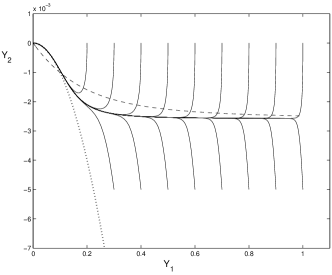
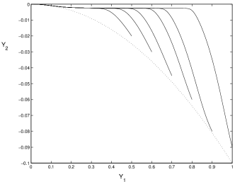
Figure 1: Phase portrait for the field $\phi$ in the re-scaled coordinates $(Y_{1},Y_{2})$ for $g_{s}=1\times 10^{-8}$ and $r_{m}=(10g_{s}/(r_{i}^{2}\lambda))^{1/2}$. The left panel show the behavior for small initial value of $Y_{2}$. The right panel shows the behavior for initial value of $Y_{2}$ close to the speed limit bound. In both panels, the dotted line corresponds to the curve that satisfies the speed limit exactly, i.e. $Y_{2}=-Y_{1}^{2}/\sqrt{\lambda}$. The dashed line in the right panel corresponds to the slow-roll approximated equation (27).

In the following we start the numerical analysis of the dynamical system. Fig.1 shows the trajectories in the phase plane $(Y_{1},Y_{2})$ with $g_{s}=1\times 10^{-8}$ and $r_{m}^{2}=10g_{s}/(r_{i}^{2}\lambda)=10^{-3}$. $Y_{1}$ will take values in the region $Y_{1c}<Y_{1}<1$; $Y_{2}$ will take values in the region $-Y_{1}^{2}/\sqrt{\lambda}<Y_{2}<Y_{1}^{2}/\sqrt{\lambda}$. We can see that there is a curve that attracts all the trajectories which correspond to the slow-roll curve. This confirms our conclusion in the last section for the specific potential (13). For all the allowed initial value, $\phi$ tends to the slow-roll curve quite soon after it begins to evolve. For simplicity, let us then analyze in detail the dynamics of $\phi$ for small initial $Y_{2}$ that satisfies $\lambda Y_{2i}^{2}/Y_{1i}^{4}\ll 1$. Since $Y_{1i}\sim 1$ and $\lambda=100$, this corresponds to $Y_{2i}\ll 10^{-1}$.

See the left panel of Fig.1 where we have taken $Y_{2i}\sim 10^{-3}$. By the numerical calculations, the dynamics of $\phi$ can be divided qualitatively into three stages. First, when it begins to evolve, it quickly evolves to the slow-roll curve. Second, it undergoes a slow-roll stage until $Y_{1}\sim 0.2$. Third, it evolves as the speed limit curve.

In the first stage, from the left panel of Fig.1, we can consistently set $Y_{1}=const.$ and because we have assumed a small initial $Y_{2}$, we can set $1-\lambda Y_{2}^{2}/Y_{1}^{4}\approx 1$. Thus from Eq.(21), $H/M=const.$ and $(H/M)^{2}\sim 10^{-1}Y_{1}^{2}$. Because $Y_{2}\sim 10^{-3}$ and $Y_{1}\sim 1$ in this stage, we have $Y_{2}^{2}/(HY_{1}/M)\ll-Y_{2}$ with $Y_{2}<0$. Thus Eq.(19) reduces to

$$Y_{2}^{\prime}=-3Y_{2}-\frac{r_{m}^{2}}{H/M}Y_{1}$$ (23)

which can be integrated to give

$$Y_{2}=(Y_{2i}+\frac{r_{m}^{2}}{3H/M}Y_{1})\exp(-3N)-\frac{r_{m}^{2}}{3H/M}Y_{1}$$ (24)

Thus in this region, $Y_{2}$ is damped exponentially to the slow-roll curve with $Y_{1}$ kept almost constant as we can see that from the upper right of the left panel. Furthermore, we can see that during the slow-roll stage, $Y_{2}\sim-r_{m}^{2}/(3H/M)$.

In the second stage, since $\lambda Y_{2}^{2}/Y_{1}^{4}\sim 10^{-3}$, we may set $1-\lambda Y_{2}^{2}/Y_{1}^{4}\approx 1$ and $Y_{2}^{\prime}\approx 0$ in the dynamical system as described by Eqs. (18), (19), and (21). Then the system can be approximated by

$$\frac{6Y_{2}^{2}}{Y_{1}}-3\frac{H}{M}Y_{2}-r_{m}^{2}Y_{1}=0$$ (25)

and

$$(\frac{H}{M})^{2}=\frac{r_{i}^{2}}{6g_{s}}r_{m}^{2}Y_{1}^{2}$$ (26)

This is a simple algebraic system of $(Y_{1},Y_{2})$ and can be solved exactly to give

$$Y_{2}=[3\frac{H}{M}-\sqrt{9(\frac{H}{M})^{2}+24r_{m}^{2}}]\frac{Y_{1}}{12}$$ (27)

The dashed line in the left panel of Fig.1 corresponds to the phase portrait of this slow-roll approximated evolution equation. Furthermore, since $(H/M)^{2}\sim 10^{-1}Y_{1}^{2}$ and $r_{m}^{2}=10^{-3}$, Eq.(27) can further reduce to

$$Y_{2}=-\frac{r_{m}^{2}}{3H/M}Y_{1}$$ (28)

This is consistent with Eq.(24).

In the third stage, when $Y_{1c}<Y_{1}<0.2$, the attractor curve coincides with the limit curve that satisfies the speed limit exactly, i.e. $Y_{2}=-Y_{1}^{2}/\sqrt{\lambda}$. This has already been pointed out in Tong as the late time behavior of $\phi$ by using the Hamilton-Jacobi method. However, as we have showed, $\phi$ will behave in this way well before it reaches the critical point $\phi_{c}$.

V Conclusions and Discussions

In this paper, we studied the cosmological dynamics of the D-cceleration scenario. We proved the inflationary attractor property using the Hamilton-Jacobi method and studied the phase portrait. Thus in this respect, this model can be a reasonable model of inflation. Of course, there are still many works needed to be done such as confrontation with observation to see whether this is a viable model of inflation.

It is interesting to ask whether the theory (1) can also be a viable candidate for quintessence which can drive an acceleration in the current universe (see, e.g. carroll-de for a recent review). This is interesting because the model building of quintessence faces the same problem as inflation: it requires the quintessence field to be in a slow-roll phase which requires a flat potential. But this is rather difficult to achieve from a particle physics point of view. So the important feature of D-cceleration, i.e. slow-roll without a flat potential, is also very attractive as a quintessence candidate. However, the problem is that, assuming we still work with the potential (13), the theory will make sense only under the condition that $\phi>\phi_{c}$. So if we want to apply this model to the late universe, we must check that $\phi$ will satisfy $\phi>\phi_{c}$ after inflation for a wide range of initial conditions. Although we still cannot present a definite answer to this question, through numerical computation, we found that the evolution of $\phi$ will be extremely slowed down before it reaches $\phi_{c}$. So this possibility still remains.

Following the same line of reasoning after the effective theory of tachyon is proposed, it is also interesting to consider the evolution of the D-cceleration in brane-world scenarios such as the well-studied Randall-Sundrum II model tachyonbrane .

References

- (1) J. E. Lidsey, astro-ph/0305528; J. E. Lidsey, D. Wands and E. J. Copeland, Phys. Rep. 337 (2000) 343; M. Gasperini and G. Veneziano, Phys. Rep. 373 (2003) 1; M. Quevedo, Class. Quant. Grav. 19 (2002) 5721 [hep-th/0210292].
- (2) S. Kachru, R. Kallosh, A. Linde, J. Maldacena, L. McAllister and S. P. Trivedi, JCAP 0310 (2003) 013 [hep-th/0308055].
- (3) E. Silverstein and D. Tong, hep-th/0310221.
- (4) D. Kabat and G. Lifschytz, JHEP 9905 (1999) 005 [hep-th/9902073].
- (5) O. Aharony, S. S. Gubser, J. M. Maldacena, H. Ooguri and Y. Oz, Phys. Rept. 323 (2000) 183 [hep-th/9905111].
- (6) A. Sen, JHEP 0204 (2002) 048; ibid, JHEP 0207 (2002) 065; M. R. Garousi, Nucl. Phys. B584 (2000) 284-299 [hep-th/0003122].
- (7) C. Armendariz-Picon, T. Damour and V. Mukhanov, Phys. Lett. B456 (1999) 209 [hep-th/9904075];
- (8) S. W. Hawking and G. F. R. Ellis, The Large Scale Structure of Space Time (Cambridge U.P., 1973).
- (9) S. M. Carroll, M. Hoffman and M. Trodden, Phys. Rev. D68 (2003) 023509 [astro-ph/0301273].
- (10) B. Carter, gr-qc/0205010.
- (11) G. W. Gibbons, Phys. Lett. B537 (2002) 1 [hep-th/0204008].
- (12) A. R. Lidde and D. H. Lyth, Cosmological Inflation and Large Scale Structure, Cambrigde University Press, 2000;
- (13) D. S. Salopek and J. R. Bond, Phys. Rev. D42 (1990) 3936; A. G. Muslimov, Class. Quant. Grav. 7 (1990) 231; J. E. Lidsey, Phys. Lett. B273 (1991) 42; A. R. Liddle, P. Parsons and J. D. Barrow, Phys. Rev. D50 (1994) 7222 [astro-ph/9408015];
- (14) Z. K. Guo, H. S. Zhang and Y. Z. Zhang, hep-ph/0309163; Zong-Kuan Guo, Y. S. Piao, R. G. Cai and Y. Z. Zhang, Phys. Rev. D68 (2003) 043508 [hep-ph/0304236]; X. H. Meng and P. Wang, Class. Quant. Grav. 21 (2004) [hep-ph/0312113];
- (15) S. M. Carroll, astro-ph/0310342.
- (16) M. C. Bento, O. Bertolami, A. A. Sen, Phys. Rev. D67 (2003) 063511 [hep-th/0208124].