New measurement on photon yields from air and the application to the energy estimation of primary cosmic rays

Abstract

The air fluorescence technique is used to detect ultra-high energy cosmic rays (UHECR), and to estimate their energy. Of fundamental importance is the photon yield due to excitation by electrons, in air of various densities and temperatures. After our previous report, the experiment has been continued using a $\@@nuc{90}{Sr}$ $\beta$ source to study the pressure dependence of photon yields for radiation in nitrogen and dry air. The photon yields in 15 wave bands between 300 nm and 430 nm have been determined. The total photon yield between 300 nm and 406 nm (used in most experiments) in air excited by a 0.85 MeV electron is 3.81$\pm$0.13 ($\pm$13 % systematics) photons per meter at 1013 hPa and 20 ^∘C. The air density and temperature dependencies of 15 wave bands are given for application to UHECR observations.

, , and

1 Introduction

In order to detect ultrahigh-energy cosmic rays (UHECR), atmospheric fluorescence light from the trajectory of the extensive air shower may be measured by mirror-photosensor systems (the fluorescence technique). In this type of experiment, the photon yield from electrons exciting air of various densities and temperatures is the most fundamental information for estimating the primary energy of UHECR. We have reported in our previous paper [1] that the photon yield between 300 nm and 406 nm in air excited by an electron with a mean kinetic energy of 0.85 MeV ($\@@nuc{90}{Sr}$ $\beta$) is 3.73$\pm$0.15($\pm$14% systematics) photons per meter at 1000 hPa and 20^∘C. We measured it with six narrow band interference filters, whose central wave lengths were 314.7, 337.7, 356.3, 380.9, 391.9 and 400.9 nm. The bandwidth of each filter at 50% of the peak transmission was about 10 nm. We estimated the photons in unmeasured wave band to be 8.8% with help from the values reported by Bunner [2]. We have also shown that the photon yields in the 337 and 358nm bands are proportional to d$E$/d$x$, when we compare our measurements with the photon yields measured at 300$\sim$1000MeV by Kakimoto et al. [3, 4].

We have made the new measurements with additional 9 filters and have improved the photon yields reported before. By comparing the measurements with filters of overlapping wavelength, the contamination of bands in the tail of each filter is estimated and corrected. In this report we provide the photon yields between 300nm and 430nm from our own measurements. The air density and temperature dependences of each wave band, and the average values in the radiative transition from the level $v^{\prime}$ to the level $v^{\prime\prime}$ in the first negative 1N(0, $v^{\prime\prime}$), and in the second positive 2P(0, $v^{\prime\prime}$), 2P(1, $v^{\prime\prime}$) and 2P(2, $v^{\prime\prime}$) systems, are given for application to UHECR observations.

In our previous report [1], we have shown the pressure dependence of the relaxation rate of the excited level of N₂ and N${}_{2}^{+}$ in nitrogen gas and in air. The radiative lifetimes $\tau_{0}$ have been obtained after determining the reference pressure $p^{\prime}$ from the pressure dependence of the photon yields (see Eqs.(5) and (10) in [1]). The definitions of $\tau_{0}$ and $p^{\prime}$ will be given in Section 3. Since there have been many experiments (e.g. [5], [6]) before the 1970s that measure $\tau_{0}$ with accuracy much better than ours, we don’t include our present measurements of $\tau_{0}$ in this article.

2 Experiment

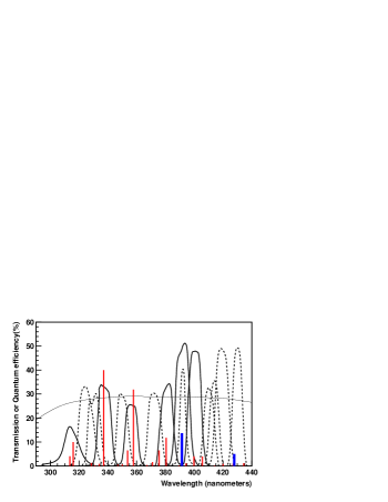
Figure 1: Typical example of quantum efficiency of PMT used (a thin solid curve) and transmission coefficients of interference filters used in the present experiment (dashed curves). Thick solid curves are those used in the previous report [1]. The relative intensities of fluorescence bands at 1000 hPa from the nitrogen molecule (thin vertical lines) and ion (broad vertical lines) in air from Bunner [2] are shown.

We chose a photon counting and thin target technique to measure the pressure dependence of photon yields (the number of photons produced by electrons per meter of travel) from nitrogen and air excited by electrons, following the method employed by Kakimoto et al. [4]. Experimental details are described in our previous report[1].

The central values of the new filters used in the present measurement are 325.0, 330.6, 350.2, 372.5, 410.0, 414.0, 418.5 and 430.0nm, and their bandwidths at half maximum are about 10nm. A measurement at 392.0nm with a band width of 4.35nm is also made. Their transmissions are indicated by dashed curves in Fig.1. The solid curves are transmissions of the filters used in the previous measurement [1]. By subtracting the contribution of bands in the tail of the transmission curves, the photon yields from 15 bands between 300 and 430nm are determined. Contributions from the 311.7, 313.6, 330.9, 333.9, 346.9, 350.0, 358.2, 367.2, 371.1, 388.4 and 389.4 nm bands can’t be separated and are included in other bands.

The systematic errors of the present experiment are discussed in [1]. Although the uncertainty from the contamination of lines in the tails of filter transmissions is reduced from 5% to 2%, the total systematic error is only reduced from 13.8% to 13%. This is because the main systematic errors are from uncertainties in the collection efficiency and quantum efficiency of the photomultiplier tubes used in the present experiment.

3 Photon yield

As described in Bunner [2] and in our previous report [1], the photon yield $\epsilon$ per unit length from gas excited by an electron is written as a function of pressure $p$ at a constant temperature $T$ in Kelvin:

$$\epsilon=\frac{p}{RT(h\nu)}\left(\frac{\mbox{d}E}{\mbox{d}x}\right)\ \left(\frac{\Phi^{\circ}}{1+\frac{p}{p^{\prime}}}\right)=\frac{Cp}{1+\frac{p}{p^{\prime}}}\ ,$$ (1)

where $R$ is the specific gas constant (N₂ : 296.9 m²s^-2K^-1 and Air : 287.1 m²s^-2K^-1) , $\displaystyle\frac{\mbox{d}E}{\mbox{d}x}$ is the energy loss in eV kg^-1 m², and $h\nu$ is the photon energy (eV). $\Phi^{\circ}$ corresponds to the fluorescence efficiency in the absence of collisional quenching. $p^{\prime}$ is the reference pressure where the lifetime of collisional de-excitation is equal to the combined lifetime, $\tau_{0}$, of the excited state for decay to any lower state, and of internal quenching.

The fluorescence efficiency for the $i$th band at pressure $p$, $\Phi_{i}(p)$, is expressed by

$$\frac{1}{\Phi_{i}(p)}=\frac{1}{\Phi_{i}^{o}}\left(1+\frac{p}{p^{\prime}_{i}}\right)\ ,$$ (2)

where $\Phi_{i}^{o}$ is $\Phi^{o}$ of the $i$th band.

The $p^{\prime}$ for nitrogen is written in terms of $\tau_{o}$ and the cross-section for nitrogen-nitrogen collisional de-excitation $\sigma_{nn}$ as

$$\frac{1}{p^{\prime}}=\frac{4\tau_{o}}{\sqrt{\pi M_{n}kT}}\sigma_{nn}\ ,$$ (3)

where $M_{n}$ is the N₂ molecular mass and $k$ is Boltzmann’s constant. $p^{\prime}$ for air is related to $\sigma_{nn}$ and the cross-section for nitrogen-oxygen collisional de-excitation $\sigma_{no}$ as

$$\frac{1}{p^{\prime}}=\frac{4\tau_{\circ}}{\sqrt{\pi M_{n}kT}}\left(f_{n}\sigma_{nn}+f_{o}\sigma_{no}\sqrt{\frac{M_{n}+M_{o}}{2M_{o}}}\right)=\frac{D}{\sqrt{T}}\ ,$$ (4)

where $M_{o}$ is the mass of oxygen molecule, and $f_{n}$ and $f_{o}$ are the fractions of nitrogen (0.79) and oxygen (0.21) in air, respectively.

It should be noted that since $p^{\prime}$ is proportional to $\sqrt{T}$, then $p^{\prime}$ at $T$, $p^{\prime}_{T}$, may be expressed by

$$p^{\prime}_{T}=p^{\prime}_{20}\sqrt{\frac{T}{293}}\ ,$$ (5)

where $p^{\prime}_{20}$ is $p^{\prime}$ at 20^∘C.

4 Analysis

4.1 Derivation of photon yields

The photon yield per unit length per electron $\epsilon$ is determined as the number of signal counts $N$ divided by the product of the following: the total number of electrons $I$, the length of the fluorescence portion $a$, the solid angle of the PMT $\Omega$, the quartz window transmission $\eta$, the filter transmission $f$, and the quantum efficiency QE and the collection efficiency CE of the PMT.

$$\epsilon=\frac{N}{I\times a\times\Omega\times\eta\times f\times\mathrm{QE}\times\mathrm{CE}}\ .$$ (6)

In the following analysis we use a value of $f$ appropriate for the main nitrogen emission band in each filter band pass. The number of photons from another band in a given filter is estimated from measurements in two adjacent filters and is subtracted from the observed photons. $I$ is about $(4\sim 5)\times 10^{8}$ from about 80 hours in each run. Finally, $\epsilon$ from a run in a vacuum is subtracted from each $\epsilon$ determined above and the corrected $\epsilon$ is determined.

4.2 Two components analysis method

In order to separate the photons from the 1N band system (427.8 nm) and the 2P band system (427.0 nm), a “two components” analysis has been performed in one filter band. The method is described in detail in our previous report [1]. Briefly, we have fitted the observed pressure dependence of $\epsilon_{\mathrm{obs}}(p)$ with a superposition of two bands in one filter by the least square(LS) method. In this case the observed photon yield $\epsilon_{\mathrm{obs}}(p)$ is the sum of the photon yields of the main band $\epsilon_{1}(p)$ and the sub-band $\epsilon_{2}(p)$, and is written as follows :

$$\epsilon_{\mathrm{obs}}(p)=\epsilon_{1}(p)+\epsilon_{2}(p) = \frac{C_{1}}{x+a_{1}}+\frac{C_{2}}{x+a_{2}}\ \ ,$$ (7)

where $x=\frac{1}{p}$, $a_{1}=\frac{1}{p^{\prime}_{1}}$ and $a_{2}=\frac{1}{p^{\prime}_{2}}$. $C_{1}$ and $p^{\prime}_{1}$ are the parameters of the main band in the filter, and $C_{2}$ and $p^{\prime}_{2}$ are those of the other band.

We determine a set of four parameters $a_{1}$, $C_{1}$, $a_{2}$ and $C_{2}$ in Eq.(7) by the LS method.

5 Results

5.1 Nitrogen

The pressure dependencies of photon yields in nitrogen gas with fourteen filters are plotted by solid circles in Fig. 2. In each figure, the main emission band in each filter band is listed. The solid curves in the figures are the best fits of Eq.(1) with $p^{\prime}$ listed in the figure. Open circles are the yields of the main band in the filter after the subtraction of other bands, which was determined by taking into account the transmission coefficients of other bands. The errors are relatively large due to the uncertainties of these subtractions. The values of $p^{\prime}$ and $C$ for each band are determined by a fit to Eq. (1) by the LS method as described in [1].

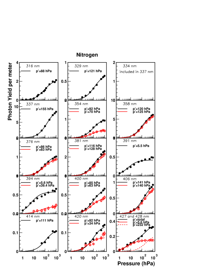
Figure 2: The pressure dependence of $\epsilon$ in N₂ at 20^∘C excited by electrons with an average energy of 0.85 MeV in 14 filters of different central wave length or different wave bands. In each figure, the main contributing line in each wave band is listed. Solid circles are the measured values. Open circles are the values after the subtraction of contamination of other emission bands. Black solid curves are the best fits of Eq.(1) to the experimental points without subtraction. Red ones are the best fits to the corrected points (open circles). In the figure labeled 427 and 428 nm, results of a two-components analysis are shown. Open circles with a solid line are from the 1N band system and the dashed line represents the 2P band system.

Table 1: Summary of the measurements of nitrogen gas. See text for detail.

main	$\epsilon$	$p^{\prime}$	$C$	$\Phi^{\circ}$
$\lambda$(nm)	m-1	hPa	$\times 10^{-2}$/(hPa$\cdot$m)	$\times 10^{-4}$
316	02.030$\pm$0.210	088.10$\pm$07.50	02.510$\pm$0.140	05.070$\pm$0.280
329	00.622$\pm$0.063	121.00$\pm$10.00	00.575$\pm$0.033	01.120$\pm$0.060
337	08.280$\pm$0.250	155.00$\pm$04.00	06.160$\pm$0.100	11.700$\pm$0.200
354	00.417$\pm$0.044	070.30$\pm$06.40	00.634$\pm$0.035	01.150$\pm$0.060
358	05.640$\pm$0.310	125.00$\pm$06.00	05.070$\pm$0.160	09.070$\pm$0.290
376	00.873$\pm$0.059	082.50$\pm$04.70	01.140$\pm$0.040	01.950$\pm$0.070
381	02.090$\pm$0.250	128.00$\pm$14.00	01.840$\pm$0.090	03.080$\pm$0.160
391	00.419$\pm$0.049	005.46$\pm$00.50	07.720$\pm$0.540	12.600$\pm$0.900
394	00.185$\pm$0.078	039.40$\pm$12.50	00.490$\pm$0.130	00.790$\pm$0.220
400	00.399$\pm$0.036	062.90$\pm$04.80	00.674$\pm$0.033	01.080$\pm$0.050
406	00.730$\pm$0.150	140.00$\pm$25.00	00.597$\pm$0.064	00.940$\pm$0.100
414	00.108$\pm$0.029	111.00$\pm$24.00	00.108$\pm$0.017	00.167$\pm$0.027
420	00.073$\pm$0.028	034.00$\pm$10.00	00.222$\pm$0.050	00.338$\pm$0.076
427	00.188$\pm$0.113	232.00${}^{+144.\phantom{0}\phantom{0}}_{-\phantom{0}71.\phantom{0}\phantom{0}}$	00.099$\pm$0.038	00.148$\pm$0.057
428	00.151$\pm$0.031	005.60$\pm$01.10	02.720$\pm$0.240	04.070$\pm$0.360
Sum	21.690$\pm$0.550	(300nm$\sim$406nm)
Sum	22.200$\pm$0.560	(300nm$\sim$430nm)

Photon yields ($\epsilon$) per meter per electron of average energy 0.85MeV in nitrogen gas at 1013 hPa and 20^∘C are determined with $p^{\prime}$ and $C$, which are listed in the third and the fourth column in Table 1. $\Phi^{\circ}$ values are also listed in the table. The total $\epsilon$ between 300 and 406 nm is 21.69$\pm$0.55, and that between 300 and 435 nm is 22.20$\pm$0.56.

5.2 Air

The pressure dependencies of photon yields in dry air, which is a mixture of 78.8% nitrogen gas and 21.1% oxygen gas, in fourteen wave bands are indicated by solid circles in Fig. 3. Open circles are the yields of the main band in the filter after the subtraction of other bands, which are estimated from measurements in neighbouring filter bands, taking into account the transmission of those lines.

Table 2: Summary of the measurements of air.

main	$\epsilon$	$p^{\prime}$	$C$	$\Phi^{\circ}$
$\lambda$(nm)	m-1	hPa	$\times 10^{-2}$/(hPa$\cdot$m)	$\times 10^{-4}$
316	0.549$\pm$0.057	023.00$\pm$01.90	2.440$\pm$0.150	04.800$\pm$0.290
329	0.180$\pm$0.026	040.20$\pm$04.60	0.465$\pm$0.042	00.880$\pm$0.080
337	1.021$\pm$0.060	019.20$\pm$00.70	5.430$\pm$0.150	10.010$\pm$0.270
354	0.130$\pm$0.022	030.60$\pm$03.90	0.437$\pm$0.046	00.769$\pm$0.080
358	0.799$\pm$0.080	018.10$\pm$01.40	4.500$\pm$0.280	07.820$\pm$0.480
376	0.238$\pm$0.036	034.10$\pm$04.10	0.722$\pm$0.068	01.200$\pm$0.110
381	0.287$\pm$0.050	019.40$\pm$02.60	1.510$\pm$0.170	02.460$\pm$0.270
391	0.302$\pm$0.020	005.02$\pm$00.26	6.040$\pm$0.250	09.600$\pm$0.390
394	0.063$\pm$0.033	024.20$\pm$09.40	0.267$\pm$0.093	00.420$\pm$0.150
400	0.129$\pm$0.019	024.20$\pm$02.80	0.544$\pm$0.053	00.847$\pm$0.082
406	0.118$\pm$0.019	012.30$\pm$01.60	0.972$\pm$0.010	01.490$\pm$0.150
414	0.041$\pm$0.009	019.30$\pm$03.40	0.217$\pm$0.031	00.327$\pm$0.047
420	0.042$\pm$0.015	007.30$\pm$01.90	0.580$\pm$0.130	00.860$\pm$0.200
427	0.032$\pm$0.023	072.00${}^{+60.\phantom{0}\phantom{0}}_{-23.\phantom{0}\phantom{0}}$	0.047$\pm$0.021	00.069$\pm$0.031
428	0.121$\pm$0.022	003.86$\pm$00.59	3.140$\pm$0.280	04.570$\pm$0.410
Sum	3.810$\pm$0.130	(300nm$\sim$406nm)
Sum	4.050$\pm$0.140	(300nm$\sim$430nm)

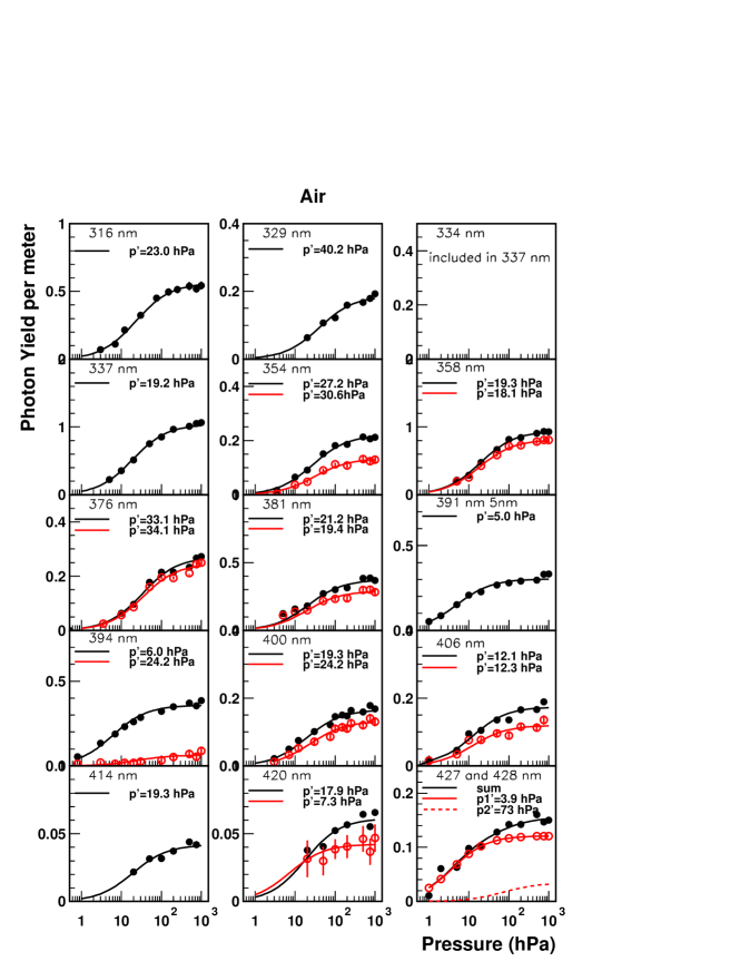
Figure 3: The pressure dependence of $\epsilon$ in air at 20^∘C excited by electrons with an average energy of 0.85 MeV in fourteen wave bands. In each figure, the main contributing band in each filter is listed. Solid circles are the measured values. Red open circles are the values after the subtraction of contamination of other bands described in the text. Black solid curves are the best fits of Eq.(1) to the experimental points. Red ones are the best fits to open circles. In the plot labeled 427 and 428 nm, the results of a two-components analysis are shown. Open circles with the solid line are from the 1N band system and the dashed line represents the 2P band system.

The values of $\epsilon$ in air at 1013 hPa and 20^∘C are determined from Eq.(1) with the best fitted values of $p^{\prime}$ and $C$. These together with $\Phi^{\circ}$ values are shown in Table 2. In estimating $\epsilon$, $C$ and $\Phi^{\circ}$, the contamination of lines in the tail of the transmission curve are subtracted from each other as mentioned before. Therefore some values listed in this table are somewhat reduced from the values in Table 9 of [1], where the measured values in each filter at 1000 hPa were listed. Total photons per meter per electron between 300 and 406nm is 3.81$\pm$0.13 and between 300 and 428nm is 4.05$\pm$0.14.

6 Discussion on experimental results

6.1 Comparison with our previous report

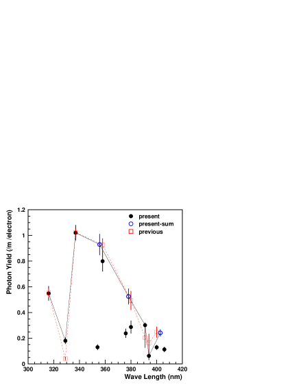
Figure 4: Comparison of the present photon yields per meter per electron (closed circles) with our previous report (open squares) [1]. Open circles are the sum of two bands which were not separated in our previous measurement.

The present results are obtained after subtracting the contamination of other bands in the tail of each filter, by comparing the measurements with another filter of overlapping wavelength. In this subtraction we have used the fitted curve to the experimental points. The photon yields at 1013 hPa in Table 1 and 2 are calculated with the best fitted values of $p^{\prime}$ and $C$. In contrast, in our previous report, the measured values at 1000 hPa are listed and the unmeasured values are estimated from the table by Bunner [2].

In Fig. 4, the present values of $\epsilon$ per meter per electron at 1013 hPa and 20^∘C are compared with the previous results. The closed circles are the present results and the open circles are the sum of two bands where they were not separated in the previous measurement. The lines are drawn to compare them easily. There are slight differences between the new and old results at 329 nm and 391 nm. In the previous report we estimated the value at 329 nm from that listed in Bunner [2], which is relatively low compared with the present measurement. Considering the 391 nm value, in the previous report we separated the 394nm band from the 391nm band by using a two components analysis, while in the present experiment the filter of the narrower bandwidth is used to separate them. Though the combined yield at 391nm and 394nm is similar, the individual values are somewhat different as seen around 391nm in Fig. 4.

6.2 Density and temperature dependence of the photon yields

The photon yields per meter by an electron of energy $E$ can be rewritten as a function of the gas density $\rho$ (in kg m^-3) and the temperature (in Kelvin) to apply to the atmosphere [4].

$$\epsilon = \frac{\left(\frac{\d E}{\d x}\right)_{E}}{\left(\frac{\d E}{\d x}\right)_{0.85\mathrm{MeV}}}\frac{A\rho}{1+\rho B\sqrt{T}}\ ,$$ (8)

where

$$A=\frac{\left(\frac{\d E}{\d x}\right)_{0.85\mathrm{MeV}}\Phi^{\circ}}{h\nu}$$ (9)

and

$$\ B=\frac{R_{air}}{p^{\prime}_{20}}\sqrt{293}\ .$$ (10)

where $R_{air}$ is the specific gas constant for air (see equation 1) . The values of $A$ and $B$ are calculated and are listed in Table 3.

Table 3: A and B values in 15 bands

main	Nitrogen		Air
$\lambda$(nm)	$A$	$B$	$A$	$B$
	m2kg-1	m3kg-1K${}^{-\frac{1}{2}}$	m2kg-1	m3kg-1K${}^{-\frac{1}{2}}$
316	21.80$\pm$1.20	00.577$\pm$0.049	20.50$\pm$1.30	02.14$\pm$0.18
329	05.00$\pm$0.29	00.419$\pm$0.035	03.91$\pm$0.35	01.22$\pm$0.14
337	53.60$\pm$0.90	00.328$\pm$0.008	45.60$\pm$1.20	02.56$\pm$0.10
354	05.52$\pm$0.31	00.723$\pm$0.066	03.68$\pm$0.39	01.60$\pm$0.21
358	44.10$\pm$1.40	00.407$\pm$0.019	37.80$\pm$2.30	02.72$\pm$0.22
376	09.95$\pm$0.35	00.616$\pm$0.035	06.07$\pm$0.57	01.44$\pm$0.17
381	16.00$\pm$0.80	00.397$\pm$0.042	12.70$\pm$1.40	02.53$\pm$0.35
391	67.20$\pm$4.70	09.310$\pm$0.860	50.80$\pm$2.10	09.80$\pm$0.51
394	04.30$\pm$1.20	01.290$\pm$0.410	02.25$\pm$0.78	02.03$\pm$0.79
400	05.87$\pm$0.28	00.808$\pm$0.061	04.58$\pm$0.44	02.03$\pm$0.23
406	05.20$\pm$0.56	00.363$\pm$0.064	08.18$\pm$0.82	03.99$\pm$0.52
414	00.94$\pm$0.15	00.460$\pm$0.100	01.83$\pm$0.26	02.55$\pm$0.45
420	01.93$\pm$0.43	01.490$\pm$0.460	04.90$\pm$1.10	06.80$\pm$1.70
427	00.86$\pm$0.33	00.220$\pm$0.100	00.40$\pm$0.18	00.68$\pm$0.38
428	23.70$\pm$2.10	09.100$\pm$1.800	26.50$\pm$2.40	12.70$\pm$1.90

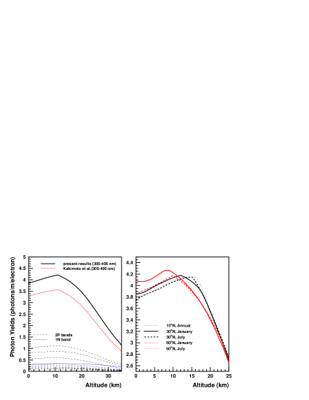
Figure 5: The altitude dependence of photon yields per meter for a 0.85 MeV electron ( between 300 and 406 nm). In the right- and left-hand figures, the US Standard Atmosphere 1976 and 1966 are assumed, respectively. In the left-hand figure, thin dashed lines are from the 2P band systems and a thin line is from the 1N band system. A thick solid line is the sum of all bands between 300 and 406 nm. The relation from Kakimoto et al. is also shown with a dotted line for wavelengths between 300 and 400 nm. The photon yields in January and July are compared in the right-hand figure at latitudes of 30^∘N and 60^∘N.

Using the values of $A$ and $B$ in Table 3, the photon yield of a 0.85 MeV electron is shown in Fig. 5 as a function of altitude. The US Standard Atmosphere 1976 [7] is assumed in the left-hand figure. Thin dashed lines are from the 2P band system and a thin solid line is from the 1N band system. A thick line shows the sum from all bands between 300nm and 406nm. The altitude dependence from Kakimoto et al. between 300 nm and 400 nm is also shown by a thick dotted line. Since the proportion of yield from the 406nm band is 3.2%, there is a difference of about 14% (300$\sim$400 nm) between ours and Kakimoto et al. independent of altitude. This is because the photon yields of Kakimoto et al. were underestimated in their unmeasured bands.

The altitude dependence of photon yields in January and July are compared in the right-hand figure for latitudes 30^∘N and 60^∘N, assuming the US Standard Atmosphere 1966 [8]. The annual value is also shown for 15^∘N. Monthly mean values of temperature and densities from CIRA 1986 (COSPAR International Reference Atmosphere) lie approximately between the lines shown for January and July at 30^∘N [9]. It would be necessary to use the several types of altitude dependence at different latitudes in experiments from space like EUSO (Extreme Universe Space Observatory) [10].

6.3 Average $p^{\prime}$ values in different radiative systems

For the radiative transition from the level $v^{\prime}$ to the level $v^{\prime\prime}$ in the 1N and 2P systems, $p^{\prime}$ values are expected to be the same for a fixed $v^{\prime}$ irrespective of $v^{\prime\prime}$, if $\Phi^{\circ}$ is much smaller than unity. So in Table 4, we summarize the average values of $p^{\prime}$, $B$ and the ratio of photon yields in nitrogen gas and air at 1013 hPa. Here weighted averages of four bands (337, 358, 381 and 406nm) for 2P(0, $v^{\prime\prime}$), five bands (316, 354, 376, 400 and 427 nm) for 2P(1, $v^{\prime\prime}$), two bands (394 and 420 nm) for 2P(2, $v^{\prime\prime}$) and two bands (391 and 428 nm) for 1N(0, $v^{\prime\prime}$) are taken for each parameter.

The present $p^{\prime}$ values are larger than those listed in Bunner [2], except 2P(0,$v^{\prime\prime}$) in air. The reason is not clear. In the next sub-section we compare the fluorescence efficiency at pressures of 100 $\sim$ 1000 hPa directly with other experiments.

Table 4: Average $p^{\prime}$ and $B$ values in different radiative systems in nitrogen gas and in air.

transition	gas	$p^{\prime}$	$B$	$\epsilon(N_{2})$/$\epsilon(air)$	$p^{\prime}$   [2]
state		hPa at 20∘C	m3kg-1K${}^{-\frac{1}{2}}$	at 1013 hPa	hPa at 27∘C
2P(0,$v^{\prime\prime}$)	N2	144.70$\pm$3.10	00.343$\pm$0.013	7.70$\pm$0.42	12000
	air	018.10$\pm$0.60	02.720$\pm$0.090		02000
2P(1,$v^{\prime\prime}$)	N2	074.50$\pm$2.80	00.628$\pm$0.03	3.43$\pm$0.29	032.6
	air	025.60$\pm$1.40	01.920$\pm$0.100		008.7
2P(2,$v^{\prime\prime}$)	N2	036.20$\pm$8.00	01.380$\pm$0.260	1.94$\pm$0.81	014.5
	air	007.90$\pm$1.80	06.200$\pm$1.400		006.1
1N(0,$v^{\prime\prime}$)	N2	005.48$\pm$0.46	09.270$\pm$0.250	1.36$\pm$0.16	001.6
	air	004.83$\pm$0.24	10.200$\pm$0.500		001.6

6.4 Comparison with other experiments

The present values of $\Phi_{i}(p)$ given by Eq.(2) in N₂ and air at $p=$800 hPa ($\sim$600 torr) are listed in Table 5, together with those of Davidson and O’Neil [11], Kakimoto et al.[3, 4] and Mitchell [12]. The values of Davidson and O’Neil are on average 2.6 times larger than ours for nitrogen, but 0.88 of ours for air. The agreement of the present results with Kakimoto et al., whose experimental conditions are similar to the present ones, is rather good both in nitrogen and in air. The efficiencies of several bands calculated from the experiment of Mitchell using X-ray photons from 0.9 to 8.0 keV [12] are also listed. Though his excitation method and the target thickness are quite different from ours, it should be noted that the efficiencies at 800 hPa for air are in fairly good agreement with each other.

Table 5: Comparison of fluorescent efficiencies $\Phi_{i}(p)$ for N₂ and air at $p$=800 hPa with those of D&O:Davidson and O’Neil [11], K:Kakimoto et al. cited from [3],[4] and M:Mitchell [12].

wave	Nitrogen				Air
length	Present	D&O	K	M	Present	D&O	K	M
nm	$\times 10^{-4}$				$\times 10^{-5}$
337	1.900$\pm$0.060	5.20	1.87	2.45	2.340$\pm$0.110	2.10	2.1	3.38
354	0.093$\pm$0.010	0.47			0.284$\pm$0.047	0.32
358	1.230$\pm$0.070	3.70	1.35		1.730$\pm$0.170	1.50	2.2
376	0.182$\pm$0.012	0.37			0.489$\pm$0.074	0.30
381	0.425$\pm$0.050	1.40		0.585	0.580$\pm$0.100	0.52		0.79
391	0.086$\pm$0.010	0.10		0.114	0.598$\pm$0.040	0.70	0.84	0.64
394	0.037$\pm$0.015				0.123$\pm$0.065	0.05
400	0.079$\pm$0.007	0.20			0.249$\pm$0.037	0.18
406	0.140$\pm$0.029	0.43		0.180	0.226$\pm$0.017	0.18		0.227
428	0.028$\pm$0.006	0.11			0.220$\pm$0.039	0.27

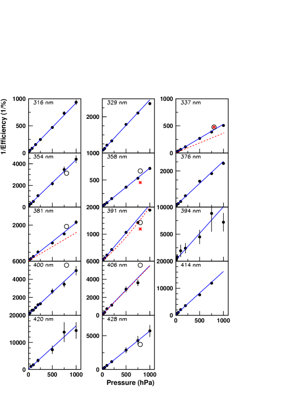
Figure 6: The reciprocal of the efficiency $\frac{1}{\Phi(p)}$ in air is plotted as a function of pressure. The best-fit functions are shown by solid lines. The relations of Mitchell [12] are shown as dashed lines in some bands. Open circles are from Davidson and O’Neil [11]. Asterisks are from Kakimoto et al. [4]

The efficiency $\Phi_{i}^{o}$ has been determined from the intercept at zero pressure of Eq.(2) in past measurements at low pressures [13]. $\frac{1}{\Phi_{i}(p)}$ for air in $\frac{1}{\%}$ is plotted as a function of pressure in Fig. 6. The results of LS fitting to Eq.(2) are shown by solid lines. The determined $\Phi_{i}^{o}$ from the intercept at zero pressure and $p^{\prime}$ from the slope are in good agreement with the values listed in Table 2. The dashed lines are from Mitchell [12]. The agreement is good for the 391 and 406 nm bands, but not good at 337 nm and 381 nm. Open circles are from Davidson and O’Neil [11] and the asterisks are from Kakimoto et al. [4]. Their agreement with the present results for the 337, 354, 358, 381, 391 and 428 nm bands are good, while there are slight differences for the 400 and 406 nm bands.

As shown in Fig. 6, the present results are in fairly good agreement with Davidson and O’Neil [11] and Mitchell [12]. The values of $p^{\prime}$ and $\Phi^{o}$ for the 391 nm band from Mitchell are in good agreement with Hirsh et al. [13] measured at low pressure. According to Mitchell, for the 391 nm band there is a significant deviation from Eq. (2) at pressures higher than 100 torr (133 hPa). This deviation results from a three-body deactivation process and can be expressed as

$$\frac{1}{\Phi(p)}=\frac{1}{\Phi^{o}}(1+Kp+Dp^{2}),$$ (11)

where $\Phi^{o}$=0.53%, $K$=1.08torr^-1 (0.810hPa^-1) and $D$=4.4$\times 10^{-4}$torr^-2 (2.48$\times 10^{-4}$hPa^-2) for the 391 nm band, which is shown by a dashed curve in the figure. Therefore we may conclude that our efficiencies at high pressures coincide with other data within experimental error, even if the present $p^{\prime}$ is different from that determined at low pressure by Hirsh et al.

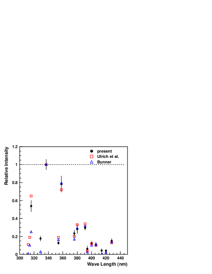
Figure 7: Relative photon intensities in air at 1013 hPa in each band between 300nm and 430 nm. The intensities are normalized to 1.0 at 337 nm.

The relative intensity of each band in air is plotted in Fig. 7 with those from Bunner [2] and Ulrich et al.[14]. The incident energies of electrons are quite different (present:0.85MeV, Ulrich et al.:15keV Bunner:mainly 50keV), but the agreement may be within the experimental error of each experiment.

We may, therefore, surely conclude that the present results can be applied to cosmic ray experiments, where photon yields at high pressures above 100 hPa are important.

7 Remarks to the energy determination of UHECR

7.1 Effects to the UHECR experiments so far

In order to estimate the effects of the present results to the energy determination of the UHECR experiments so far made, let us compare the observed number of photons from the extensive air showers using the present photon yields with those used by the HiRes experiment [15]. The HiRes experiment currently uses a combination of results from Kakimoto et al. [4] and Bunner [2].

The conditions for the present calculation are similar to a previous one [16] and are summarized below.

• Air shower simulation code used: CORSIKA 6.020 [17, 18] with QGSJET model [19].

  • Primary particle=proton

  • Energy $E$=$10^{19}$eV and $10^{20}$eV

  • Zenith angle $\theta=0$ and 60^∘ (In the case of $\theta=60^{\circ}$, the shower axis is on the plane perpendicular to the line of sight.)

  • In each combination of above parameters, 30 events are simulated to get the average longitudinal development curve.

• The number of emitted photons is calculated from the total energy deposit of shower particles, $\Sigma$d$E$/d$x$, in each step for sampling of longitudinal development, using Eq. (8). The energy release provided by CORSIKA was used for this calculation, in which the contribution by particles below simulation energy threshold is carefully taken into account [20].

• The observation height is 0 m a.s.l.

• Emitted photons in each step width of depth are attenuated by Rayleigh scattering with the following transmission factor

  $$T_{R}=\exp\left[-\frac{|x_{1}-x_{2}|}{X_{R}}\left(\frac{400\mathrm{[nm]}}{\lambda}\right)^{4}\right],$$ (12)

  where $X_{R}$=2974 g/cm², and $x_{1}$ and $x_{2}$ are the slant depths of two points.

• Photons are attenuated by Mie scattering with

  $$T_{M}=\exp\left(\frac{H_{M}}{L_{M}\cos\theta}\left[\exp\left(-\frac{h_{1}}{H_{M}}\right)-\exp\left(-\frac{h_{2}}{H_{M}}\right)\right]\frac{400\mathrm{[nm]}}{\lambda}\right),$$ (13)

  where scale height $H_{M}=1.2$km and the horizontal attenuation length $L_{M}=25$km. $h_{1}$ and $h_{2}$ are the heights of the emission point and the detection point of the light, respectively.

• Total number of observed photons is calculated by adding photons from each step of depth.

• US standard atmosphere 1976[7] is used for the altitude dependences of density and temperature.

• Wavelength dependences of the HiRes filter transmission and quantum efficiency (QE) of the HiRes Photomultiplier tube (PMT) are taken into account in some cases.

Figure 8: Comparison of observed total photon number in various conditions. $R_{N}=\frac{N_{HiRes}}{N_{present}}$ is plotted as a function of distance. (a) The effect of the primary energy for the showers with $\theta=0^{\circ}$. Circles with a solid line are for $\log E(\mathrm{eV})=20$ and triangles with a dashed line for $\log E(\mathrm{eV})=19$. Only Rayleigh scattering is taken into account. (b) The effect of zenith angle for $\log E=20$. Only Rayleigh scattering is taken into account. A solid line is for $0^{\circ}$ and a dashed line for $60^{\circ}$. (c) The effect of Mie scattering for $\log E=20$ and $\theta=0^{\circ}$. Circles are for the case that only Rayleigh scattering is taken into account, while triangles are for the case that Mie scattering is also considered. (d) The case of HiRes filter transmission and PMT QE for the showers with $\log E=20,\theta=0^{\circ}$. Both Rayleigh and Mie scatterings are taken into account. Circles are the same with those in (c).

In Fig.8, the ratios $R_{N}$ of the number of total observed photons with the HiRes photon yields ($N_{HiRes}$) to that with the present ones ($N_{present}$) are plotted for various conditions as a function of distance (horizontal distance to the 2 km point a.s.l. along the shower track). $N_{HiRes}$ is smaller than $N_{present}$ by $-11$% to $-15$% depending on the distance to the shower due to Rayleigh scattering (Fig.8 (a)). In the case of the inclined shower, the change of $R_{N}$ with distance is smaller than for the case of the vertical shower, and the difference is between $-11$% and $-13$% (Fig.8(b)). $R_{N}$ changes little if we include the effect of Mie scattering (with its weak wavelength dependence) (Fig.8(c)) and is almost independent of the primary energy (Fig.8(a)). However, if the HiRes filter transmission and the QE of the PMT are taken into account, $R_{N}$ becomes closer to unity, $-4$% to $-7$%, depending on the distance (Fig.8(d)). This is because the transmission coefficient of the broad band filter used in HiRes drops below 320nm and above 380nm where the difference of photon yields between the present experiment and those assumed by HiRes are relatively large.

We need more a detailed analysis based on the experimental conditions to infer the individual energy estimation of cosmic rays, taking into account the wavelength dependent items (photon yields, scattering effects, detector performance, etc.).

7.2 Application of the present photon yields

In UHECR fluorescence experiments, the primary energy is estimated from the calorimetric energy, $E_{cal}$, with a correction for missing energy, $E_{miss}$, that carried by neutrinos and muons, and that lost due to nuclear excitation [21]. $E_{cal}$ may be determined from the experiment from the path-length integral multiplied by the mean ionization loss rate, $\alpha$, over the entire shower as

$$E_{cal}=\alpha\int^{\infty}_{0}N_{ch}(X)\mathrm{d}X\ ,$$ (14)

where $N_{ch}(X)$ is the number of charged particles in the shower as a function of atmospheric depth $X$ in g/cm². Song et al. [21] showed that this technique provides a good estimate of the primary energy of cosmic rays with $\alpha$=2.19 MeV/(g/cm²) by using the CORSIKA air shower simulation program.

Their arguments would be accepted as far as $N_{ch}(X)$ can be determined unambiguously. In practice, however, it is not straightforward to convert the observed number of photons for each angular bin in the camera of the detector to $N_{ch}(X)$. This is because the photon yield depends on the temperature and density of air along the trajectory of the electrons, and most particles of low energies are not traveling parallel to the shower axis. Alvarez-Muñiz et al. [22] studied the ratio of the average track length traveled by the shower particles in a some depth interval and that projected onto the shower axis. They showed that the ratio depends on the shower age and is 1.18 at shower maximum. That is, $E_{cal}$ is possibly overestimated, if Eq. (14) is used without path length correction.

Instead of estimating $N_{ch}(X)$, Dawson [15] has proposed to use the energy deposited in the atmosphere by the shower per g/cm² of depth. This is determined from the number of photons, $L(X)$, after correcting the attenuation of photons due to Rayleigh and Mie scattering and subtracting Cherenkov contamination. That is, the energy deposited by the shower in the grammage interval $\Delta X$, $\Delta E_{dep}(X)$, is expressed by

$$\frac{\Delta E_{dep}(X)}{\Delta X}=\frac{1}{\Delta X}\sum_{i}\left(\frac{L_{i}(X)(h\nu)_{i}}{\Phi_{i}(X)}\right),$$ (15)

where $L_{i}(X)$ is the fraction of the flux $L(X)$ in different wavelength bin $i$ and $(h\nu)_{i}$ is the photon energy of bin $i$.

Then the calorimetric energy is estimated from

$$E_{cal}=\int^{\infty}_{0}\frac{\Delta E_{dep}(X)}{\Delta X}\mathrm{d}X\ ,$$ (16)

It would be much more realistic to use Eqs. (15) and (16) to estimate the primary energy. $\Phi_{i}(X)$ is a function of pressure (=$\rho R_{Air}T$) at depth $X$ and is expressed by Eq. (2). Recommended values of $\Phi_{i}^{\circ}$ and $p^{\prime}$ are listed in Table 2 for each wavelength.

8 Conclusion

Photon yields have been measured in fifteen wave bands as a function of pressure, for nitrogen and dry air excited by electrons of an average energy of 0.85 MeV. The pressure dependencies of 15 wave bands between 300 nm and 430 nm have been determined with our own measurements. The total photon yields between 300 nm and 430 nm are 22.20$\pm$0.56 and 4.05$\pm$0.14 per meter per electron at 1013 hPa and 20^∘C for nitrogen and air, respectively. If we restrict the wave bands up to 406 nm, the corresponding values are 21.69$\pm$0.55 and 3.81$\pm$0.13. The systematic error in the measurement is 13 %.

From the pressure dependence of photon yields, their temperature and density dependencies of each band are determined for application to the energy estimation of UHECRs by the fluorescence method. It would be much more realistic to use energy deposition rather than the number of charged particles for each angular bin in the camera of the detector to estimate the primary energy. $\Phi_{i}^{\circ}$ and $p^{\prime}$ in each wavelength are given in Table 2 for application to estimate the energy deposition.

References

- [1] M. Nagano, K. Kobayakawa, N. Sakaki and K. Ando, Astroparticle Physics, 20 (2003) 293.
- [2] A.N. Bunner, Ph.D. thesis (Cornell University) (1967).
- [3] S. Ueno, Master thesis (Tokyo Institute of Technology), (1996) (in Japanese).
- [4] F. Kakimoto, E.C. Loh, M. Nagano, H. Okuno, M. Teshima and S. Ueno, Nucl. Instrum. Methods Phys. Res., A372 (1996) 244.
- [5] J.E. Hesser, J. Chemical Physics, 48 (1968) 2518.
- [6] L.W. Dotchin, E.L. Chupp and D.J. Pegg, J. Chemical Physics, 59 (1973) 3960.
- [7] U.S. Standard Atmosphere 1976, U.S. Government Printing Office (Washington D.C., 1976).
- [8] U.S. Standard Atmosphere Supplements,1966, U.S. Government Printing Office (Washington D.C., 20402).
- [9] From the slide shown by V. Rizi at the Workshop Airlight 03, December (2003). http://www.auger.de/events/air-light-03/index.html
- [10] EUSO Report on the Phase-A Study, EUSO-PI-005-1 (ed. by L. Scarsi et al.) (2004).
- [11] G. Davidson and R. O’Neil, J. Chem. Phys. 41 (1964) 3946.
- [12] K.B. Mitchell, J. Chem. Phys. 41 (1970) 1795.
- [13] M.N. Hirsh, E. Poss and P.N. Eisner, Phys. Rev. A 1 (1970) 1615.
- [14] From the slide shown by A. Ulrich at the Workshop Airlight 03, December (2003). http://www.auger.de/events/air-light-03/index.html
- [15] B. Dawson, http://www.auger.org/admin/GAP-2002-067 (2002).
- [16] N. Sakaki, M. Nagano, K. Kobayakawa and K. Ando, Proc. Int. Cosmic Ray Conf. (Universal Academy Press, Inc., Tokyo) (2003) 841.
- [17] D. Heck, J. Knapp, J.N. Capdevielle, G. Schatz, and T. Thouw, Report FZKA 6019 (1998), Forschungszentrum Karlsruhe; http://www-ik.fzk.de/~heck/corsika/physics_description/corsika_phys.html
- [18] D. Heck and J. Knapp, Report FZKA 6097 (1998), Forschungszentrum Karlsruhe
- [19] N.N. Kalmykov, S.S. Ostapchenko and A.I. Pavlov, Nucl. Phys. B (Proc. Suppl.), 52B (1997) 17.
- [20] M. Risse and D. Heck Astroparticle Physics, 20 (2004) 661.
- [21] C. Song, Z. Cao, B.R. Dawson, B.E. Fick, P. Sokolsky and X. Zhang, Astroparticle Physics, 14 (2000) 7.
- [22] J. Alvarez-Muñiz, E. Marqués, R.A. Vázquez and E. Zas, Phys. Rev D, 67 (2003) 101303(R).