Oscillation frequencies and mode lifetimes in $\alpha$ Centauri A

Abstract

We analyse our recently-published velocity measurements of $\alpha$ Cen A (Butler et al. 2004). After adjusting the weights on a night-by-night basis in order to optimize the window function to minimize sidelobes, we extract 42 oscillation frequencies with $l=0$–3 and measure the large and small frequency separations. We give fitted relations to these frequencies that can be compared with theoretical models and conclude that the observed scatter about these fits is due to the finite lifetimes of the oscillation modes. We estimate the mode lifetimes to be 1–2 d, substantially shorter than in the Sun.

1 Introduction

Its proximity and its similarity to the Sun have made $\alpha$ Cen A a prime target for asteroseismology. The first clear detection of p-mode oscillations was made by Bouchy & Carrier (2001, 2002) using velocity measurements with the CORALIE spectrograph over 13 nights. These results confirmed the earlier but less secure detection by Schou & Buzasi (2000), who used photometry from the WIRE satellite. Based on the CORALIE data, Bouchy & Carrier (2002) published frequencies for 28 modes with $l=0$–$2$ and $n=15$–$25$ and these have been compared with theoretical models by Thévenin et al. (2002) and Thoul et al. (2003). Meanwhile, oscillations in $\alpha$ Cen B have been reported by Carrier & Bourban (2003), adding to the growing list of stars in which solar-like oscillations have been detected – see Bedding & Kjeldsen (2003) for a recent review.

We recently reported observations of $\alpha$ Cen A made over 5 nights in both Chile with UVES and in Australia with UCLES (Butler et al., 2004, hereafter Paper I). These observations covered a shorter time span than those by Bouchy & Carrier but had substantially better velocity precision and the benefit of two-site coverage.

In Paper I we described the method used to process the velocity measurements. In brief, we first removed slow drifts and sudden jumps of a few metres per second, presumably instrumental, from each time series. We then used the measurement uncertainties as weights in calculating the power spectrum (according to $w_{i}=1/\sigma_{i}^{2}$), but we found it necessary to modify some of the weights to account for a small fraction of bad data points. In the end, we reached a noise floor of 2.0 cm s^-1 in the combined amplitude spectrum. In this paper, we extract oscillation frequencies, measure the large and small frequency separations and also estimate the mode lifetimes.

2 Optimizing the window function

The observing window contains gaps due to day time and bad weather, which means that each peak in the power spectrum is accompanied by sidelobes. This can be quantified by calculating the spectral window, which is the power spectrum of the observing window and is shown in Fig. 6 of Paper I. The two-site coverage of our observations means that the gaps are relatively small in the latter part of the run, when the weather was best. However, as discussed in Paper I, the UVES data have much higher weight than the UCLES data, due to their higher precision. This means that the spectral window, which takes the weights into account, has quite strong sidelobes (24% in power). As is well known, these sidelobes complicate the oscillation spectrum, especially for weaker modes, for which the interaction between noise and signal can cause sidelobes to become higher than the central peak and lead to mis-identifications.

To address this problem, we have adjusted the weights on a night-by-night basis in order to optimize the window function. To be specific, we allocated separate adjustment factors to each of the three UVES nights and the five UCLES nights. The weights on each night were multiplied by these factors and the spectral window was calculated, and this process was iterated to minimize the height of the sidelobes. The final values for these weight multipliers were 0.88, 1.00 and 1.12 for the three UVES nights and 0.11, 0.42, 3.25, 8.19 and 7.62 for the five UCLES nights. We treated separately the short period of overlap (see Paper I), and the weight multiplier for that period turned out to be 1.39.

This optimization process has significantly increased the weight given to the last three UCLES nights, which makes sense because these fill in the gaps in the UVES data. The power spectrum based on these adjustment factors is shown in Fig. 1. The resulting spectral window is shown in the inset, and the highest sidelobes are only 3.6% in power. The optimization process has slightly degraded the frequency resolution, with the FWHM of the spectral window increasing from 3.85 $\mu$Hz to 4.13 $\mu$Hz. However, the main trade-off is an increase in the noise floor in the amplitude spectrum at high frequencies, from 2.0 to 2.9 cm s^-1. Nevertheless, we have found that the improvement in the spectral window makes the oscillation spectrum much clearer, and this compensates for the reduction in signal-to-noise. We note that we found similar results to those reported here when we performed the analysis using a compromise weighting scheme, in which we used the square roots of the weight multipliers given above.

3 Frequency analysis

The large separation of $\alpha$ Cen A was measured to be $\sim 106\,$$\mu$Hz by Schou & Buzasi (2000) and Bouchy & Carrier (2001). In Fig. 2 we show the central part of our power spectrum (2020–2970 $\mu$Hz) folded with a spacing of $\Delta\nu=106.2$ $\mu$Hz. We can clearly see peaks corresponding to modes with degree $l=0,1,2$ and $3$. In Fig. 3 we show the power spectrum in echelle format, where we have smoothed in the vertical direction to make the ridges more visible. Again, four ridges corresponding to $l=0$–$3$ are visible.

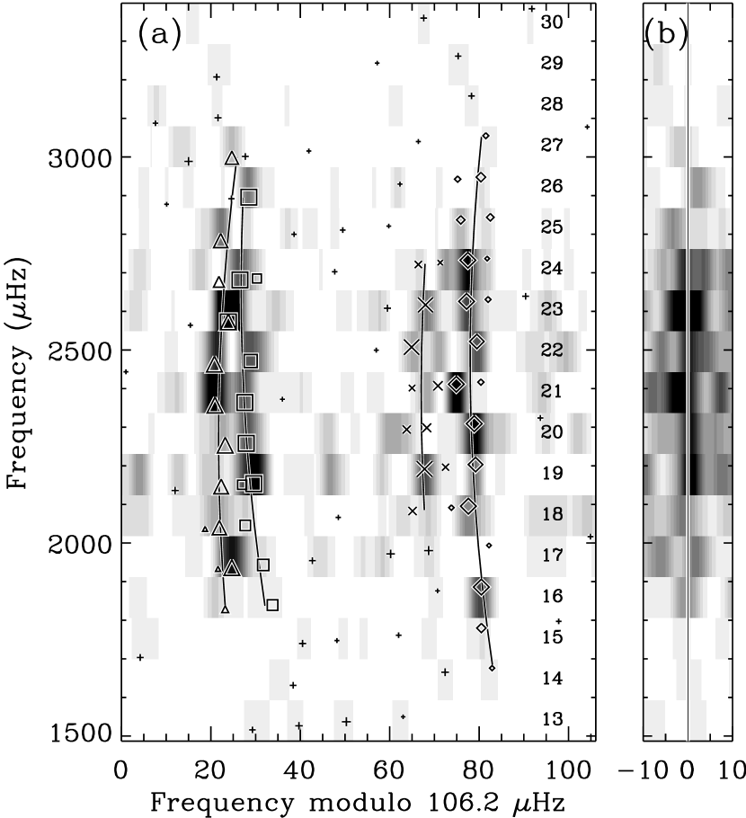
Figure 4: (a) The greyscale shows the power spectrum in echelle format (without smoothing) and the symbols show the peaks extracted by iterative sine-wave fitting: $l=0$ (squares), $l=1$ (diamonds), $l=2$ (triangles), $l=3$ (crosses) and other peaks (plus signs). The sizes of the symbols are proportional to the amplitudes of the peaks. The curves show fits to the frequencies, as described in the text, and the numbers up the right side show the $n$ value of each order. (b) The power summed over the four ridges ($l=0$–3) after first subtracting from each one the frequency predicted by equations (4)–(7).

The next step was to measure the frequencies of the strongest peaks in the power spectrum, which we did in the standard way using iterative sine-wave fitting. These frequencies are given in Table 1 and are shown as symbols in Fig. 4(a), over-plotted on a grey scale of the power spectrum itself (this time without any smoothing). The sizes of the symbols indicate the strengths of the peaks (the amplitudes are given in Table 2). We have assigned $l$ values to the strongest peaks, based on their location in the echelle diagram. The four curves are fits to the data and are described below.

There is a significant scatter of the individual peaks about each ridge, which we interpret as reflecting the finite lifetime of the oscillation modes. In several cases, the iterative sine-wave fitting has produced two peaks that appear to represent a single oscillation mode, which is to be expected if we have partially resolved the modes (see Sec. 4 for further discussion of the mode lifetimes). In these cases, both peaks are shown in Fig. 4(a) but in Tables 1 and 2 (and also in Fig. 5) they are combined into a single weighted mean. It is also important to note that the separation between $l=0$ and $l=2$ is not well resolved by our observations, and in one case (2572.7 $\mu$Hz) it seems that the two modes have combined to form a single peak.

To show the power spectrum more clearly, we have plotted it on an expanded scale in Fig. 5 and indicated the extracted frequencies. Note that interference between noise peaks, oscillation peaks and their sidelobes has created apparent mismatches in a few places between the peaks in the power spectrum and the dotted lines representing the extracted frequencies. Such interference is relatively minor given the low level of both noise and sidelobes, but it is still significant (and it is, of course, the reason we chose to extract frequencies using the iterative fitting process). Also, as mentioned above, the iterative fitting has sometimes produced two peaks that have been averaged into a single value for this figure.

Asteroseismology involves comparing observed frequencies with theoretical models, and the values listed in Table 1 could be used for that purpose. However, the scatter caused by the finite mode lifetimes means that we would do better to fit to the ridges, in order to obtain more accurate estimates for the eigenfrequencies of the star. We now describe the procedure that we used to perform this fit, which begins with an examination of the small frequency separations.

Figure 6(a) shows our measured values for the three small separations, which are defined according to the usual conventions (for a recent review, see Bedding & Kjeldsen, 2003). Thus, $\delta\nu_{02}$ is the separation between adjacent peaks with $l=0$ and $l=2$ and $\delta\nu_{13}$ is the separation between $l=1$ and $l=3$. The third small separation, $\delta\nu_{01}$, is the amount by which $l=1$ modes are offset from the midpoint between the $l=0$ modes on either side. Since one could equally well define $\delta\nu_{01}$ to be the offset of $l=0$ modes from the midpoint between consecutive $l=1$ modes, we have shown both versions in Fig. 6(a).

The observations show that the small separations in $\alpha$ Cen vary with frequency, as was already reported for $\delta\nu_{02}$ by Bouchy & Carrier (2002). We have fitted straight lines to each of the three separations (fitting a polynomial of higher degree is not justified by the data). These lines are shown in Fig. 6(a) and the equations are as follows:

$$\delta\nu_{02} = ~{}~{}5.46\,\mbox{$\mu$Hz}\;-\;0.0060\;(\nu-2400\,\mbox{$\mu$Hz})$$ (1)

$$\delta\nu_{13} = 10.99\,\mbox{$\mu$Hz}\;-\;0.0012\;(\nu-2400\,\mbox{$\mu$Hz})$$ (2)

$$\delta\nu_{01} = ~{}~{}2.41\,\mbox{$\mu$Hz}\;-\;0.0029\;(\nu-2400\,\mbox{$\mu$Hz})$$ (3)

Using these fits, we were then able to adjust the measured frequencies to remove the effect of the small separations and so align them all in a single ridge. The result is shown in Fig. 6(b). Note that we have taken the frequencies modulo $\Delta\nu/2$, so that the even ($l=0$, 2) and odd ($l=1$, 3) ridges are superimposed. To this single ridge we then fitted a parabola (the highest degree polynomial that is justified by the data), which is shown in the figure.

This completes our fit to the observed frequencies, which has involved nine free parameters (three linear fits and one parabola). We show this fit and the observed frequencies in Fig. 6(c), and also in Fig. 4(a). The equations for this fit are as follows:

$$\nu_{n,0} = \left(2363.85+105.70\;(n-21)+0.088\;(n-21)^{2}\right)\,\mbox{$\mu$Hz}$$ (4)

$$\nu_{n,1} = \left(2414.35+106.10\;(n-21)+0.088\;(n-21)^{2}\right)\,\mbox{$\mu$Hz}$$ (5)

$$\nu_{n,2} = \left(2464.60+106.52\;(n-21)+0.088\;(n-21)^{2}\right)\,\mbox{$\mu$Hz}$$ (6)

$$\nu_{n,3} = \left(2509.70+106.41\;(n-21)+0.088\;(n-21)^{2}\right)\,\mbox{$\mu$Hz}.$$ (7)

These relations, rather than the actual frequencies, should be used when comparing with theoretical models because the measured frequencies are significantly affected by the mode lifetime. Note that these relations should not be extrapolated to frequencies beyond those actually measured. The formal uncertainties on the frequencies given by these relations are shown in Fig. 6(d), based on the uncertainties in the parameters of the parabola that was fitted in Fig. 6(b). Over most of the range the uncertainty is 0.3–0.4 $\mu$Hz, rising to about 0.8 $\mu$Hz at the ends.

To examine whether the oscillations frequencies deviate systematically from equations (4)–(7), we have used those equations to “straighten” the ridges. Figure 4(b) shows the result, where we have summed the power of the four ridges ($l=0$–3) after first subtracting from each the frequency predicted by equations (4)–(7). Looking at the highest frequencies (above 3000 $\mu$Hz), there seems to be evidence for a departure from the fit in the sense that the ridge of power curves to the left. More observations are needed to confirm this result.

Another useful parameter to compare with models is the large separation, $\Delta\nu$. The measured values are shown in Fig. 6(e) and there is an upward trend with frequency that was previously noted by Bouchy & Carrier (2002) and which is responsible for the curvature in the echelle diagram. The line in Fig. 6(e) shows the large separation for $l=1$ calculated from equation (5). Lines for other $l$ values (not shown) are almost indistinguishable.

The small solid circles in Fig. 6(c) show the 28 frequencies reported by Bouchy & Carrier (2002). Note these are all $l=0$–$2$ because those observations were single-site and aliases prevented the detection of $l=3$. On the other hand, our observations were shorter, which made it more difficult to separate $l=0$ from $l=2$. Keeping in mind the scatter induced by the finite mode lifetimes, the agreement between the two results is excellent, especially for $l=1$.

4 Mode lifetimes

As already mentioned, the observed frequencies show a significant scatter about the fitted relations. If the modes were coherent (i.e., pure sinusoids with infinite lifetimes), we have shown using simulations that we would be able to measure them with a typical accuracy of 0.4 $\mu$Hz or better. The observed scatter is much greater than this, which we interpret as reflecting the finite lifetimes of the oscillation modes. As is well established for the Sun, the power spectrum of a stochastically excited oscillation that is observed for long enough will display a series of closely spaced peaks under a Lorentzian profile, the width of which indicates the mode lifetime (e.g., Toutain & Fröhlich, 1992). If, as in this case, the observations are not long enough to resolve the Lorentzian profile then the effect of the finite mode lifetime is to randomly shift each oscillation peak from its true position by a small amount. This is responsible for the scatter observed in Fig. 6.

Measuring this scatter gives us an opportunity to estimate the mode lifetime in $\alpha$ Cen A. In Table 3 we give the scatter of the observed frequencies about the fit for two frequency ranges (a finer subdivision in frequency is not justified by the data). We have converted these to mode lifetimes using simulations, as follows. We simulated a single oscillation mode, sampled with the same window function and weights as the actual observations. We used the method described by Stello et al. (2004) to simulate an oscillation that was re-excited continuously with random kicks and damped on a timescale that was an adjustable parameter (the mode lifetime). For a given mode lifetime, we created 100 simulated time series that differed only in the random number seed. For each one we measured the position of the peak in the power spectrum and hence determined the scatter of the “observed” frequency about its true value. This was repeated for different values of the mode lifetime, allowing us to calibrate the relationship between the mode lifetime and the scatter in the observed frequencies. The inferred mode lifetimes for $\alpha$ Cen A are given in Table 3.

To check this technique, we also analysed segments of an 805-day series of full-disk velocity observations of the Sun taken by the GOLF instrument on the SOHO spacecraft (Ulrich et al., 2000). We sampled these data with the same window function and weights as the $\alpha$ Cen A observations, and extracted the frequencies of the strongest 30 oscillation peaks using the same iterative sine-wave fitting method as for $\alpha$ Cen A (see Section 3). We compared these frequencies with the values measured by Thiery et al. (2000) from the full 805-day GOLF series, and thereby determined the scatter on our “observed” solar frequencies. We then used the calibration derived from the simulations, as described in the previous paragraph, to infer mode lifetimes. The results for two frequency ranges are given in Table 3. In this case, we were able to compare these mode lifetimes with published values. For this we took values measured by Chaplin et al. (1997) from fitting Lorentzian profiles to a 32-month power spectrum of ground-based solar velocities. We see that our method reproduces the published lifetimes within the uncertainties, confirming the validity of the technique.

Our main result is that mode lifetimes for $\alpha$ Cen A are 1–2 d, significantly shorter than the values of 3–4 d found in the Sun. Is this result consistent with the results for $\alpha$ Cen A presented by Bouchy & Carrier (2002)? Their frequencies were measured from a time series of considerably longer duration than ours (12.4 d versus 4.6 d), so we would expect them to have lower scatter. This is indeed the case – we measure a scatter of about 0.8 $\mu$Hz from their frequencies. This is much greater than would be expected for coherent oscillations (about 0.1–0.2 $\mu$Hz), but is consistent with the mode lifetime that we measured from our observations.

Note that the mode lifetime $\tau$ is related to the FWHM $\Gamma$ of the corresponding Lorentzian via $\tau=1/(\pi\Gamma)$. Thus, if $\alpha$ Cen A were observed for long enough, we would expect each mode to generate a Lorentzian profile in the power spectrum with width $\Gamma=2$–3 $\mu$Hz. This is less than the FWHM of 4 $\mu$Hz of the spectral window of our observations, which explains why such a profile is not apparent in our power spectrum.

We have assumed that the scatter of the observed frequencies about a smooth trend is due to the effects of the finite mode lifetime. However, we should also consider that the actual eigenfrequencies of the star may have small deviations from regularity. For the Sun, this is indeed the case, but at a low level: the frequencies reported by Thiery et al. (2000) deviate from a parabola in the echelle diagram by 0.2–0.3 $\mu$Hz. If $\alpha$ Cen A possesses irregularities of this magnitude, their contribution to the scatter that we measured is very small. Correcting for this would lead us to reduce the values of scatter in Table 3 by about 0.02 $\mu$Hz, and to increase the estimates of mode lifetimes by a few percent. We conclude that such frequency deviations have negligible effect on our measurements of the mode lifetime.

5 Conclusions

We have analysed the two-site observations of $\alpha$ Cen A that were described in Paper I. Our main results are as follows:

1. By adjusting the weights for each night, we optimized the window function and reduced the sidelobes in the spectral window to only 3.6% in power. This allowed us to measure the frequencies of the strongest peaks in the power spectrum using iterative sine-wave fitting, without any ambiguities from daily aliases.

2. We clearly detected several modes with $l=3$, the first time this has been achieved for solar-like oscillations.

3. We made fits to the measured frequencies and obtained the relations in equations (4)–(7). Given the significant scatter in the frequencies, we suggest that comparison with theoretical models is best done via these fitted relations.

4. Based on the scatter of the observed frequencies, we inferred mode lifetimes in $\alpha$ Cen A of 1–2 d. These shorter-than-expected lifetimes present a challenge to theoretical models (Houdek et al., 1999), and also raise concerns for asteroseismology because they degrade the precision with which oscillation frequencies can be measured. It is clear that more stars need to be observed before we can determine how this important parameter varies in the H-R diagram.

Figure 1: Power spectrum of the combined $\alpha$ Cen A velocity time series, with weights for each night adjusted to optimize the window function. The inset shows the spectral window (power in arbitrary units), with the frequency scale expanded by a factor of 5.

Figure 2: The power spectrum of $\alpha$ Cen A folded at the large separation, showing peaks corresponding to $l=0$–3.

Figure 3: The power spectrum of $\alpha$ Cen A in echelle format, and smoothed slightly in the vertical direction. The column of numbers on the right shows the $n$ value of each order.

Figure 5: Power spectrum of $\alpha$ Cen A with mode frequencies overlaid. Same as Fig. 1, but on an expanded scale and with the frequencies in Table 1 marked by dotted lines.

Figure 6: (a) The three small separations as a function of frequency. Symbols connected by dotted lines show the measured values: $\delta\nu_{02}$ (triangles), $\delta\nu_{13}$ (crosses) and $\delta\nu_{01}$ (two sets of squares). The three solid lines are lines of best fit. (b) The frequencies after adjusting by subtracting off the small separations, to align them in in a single ridge. The curve is the parabola of best fit. (c) The measured frequencies (unadjusted) in echelle format. The curves show the four parabolas defined by equations (4)–(7), and the small solid circles show the frequencies reported by Bouchy & Carrier (2002). (d) Formal uncertainty in the fit as a function of frequency. (e) The large separation as a function of frequency for the four values of $l$, where the line shows the separation for $l=1$ calculated from equation (5). In panels (b), (c) and (e) the symbols indicate $l$ values, with the same meaning as in Fig. 4.

Table 1: Oscillation frequencies for $\alpha$ Cen A ($\mu$Hz)

$n$	$l=0$	$l=1$	$l=2$	$l=3$
14	…	1675.9	…	…
15	…	1779.7	1828.6	…
16	1839.2	1885.9	1935.7	…
17	1943.3	1993.8	2038.9	2082.9
18	2045.5	2094.6	2146.3	2193.1
19	2152.9	2203.2	2253.4	2296.3
20	2258.1	2309.1	2357.3	2404.8
21	2364.0	2412.4	2463.4	2507.5
22	2471.5	2522.1	2572.7	2616.8
23	2572.7	2627.1	2676.8	2723.5
24	2682.7	2733.2	2783.4	…
25	…	2840.2	…	…
26	2895.9	2945.7	2998.3	…
27	…	3055.1	…	…

Table 2: Oscillation amplitudes for $\alpha$ Cen A (cm s^-1)

$n$	$l=0$	$l=1$	$l=2$	$l=3$
14	…	6.5	…	…
15	…	11.8	8.8	…
16	13.5	25.0	30.2	…
17	14.4	5.9	19.1	10.6
18	13.3	24.9	18.7	24.8
19	34.0	18.6	21.3	15.2
20	20.7	31.3	31.8	14.4
21	21.1	31.6	27.1	19.6
22	16.7	18.5	40.3	18.9
23	40.3	26.2	13.9	11.2
24	27.8	30.5	18.0	…
25	…	14.4	…	…
26	21.4	14.4	16.8	…
27	…	7.5	…	…

Table 3: Mode lifetimes in $\alpha$ Cen A and the Sun

	Frequency	Scatter	Inferred	Published
	($\mu$Hz)	($\mu$Hz)	lifetime (d)	lifetime (d)
$\alpha$ Cen A	1700–2400	1.50 $\pm$ 0.23	1.4${}^{\scriptscriptstyle{+0.5}}_{\scriptscriptstyle{-0.4}}$
	2400–3000	1.60 $\pm$ 0.25	1.3${}^{\scriptscriptstyle{+0.5}}_{\scriptscriptstyle{-0.4}}$
Sun	2400–3050	0.95 $\pm$ 0.17	4.0${}^{\scriptscriptstyle{+2.0}}_{\scriptscriptstyle{-1.1}}$	3.17 $\pm$ 0.15
	3050–3700	1.31 $\pm$ 0.23	2.0${}^{\scriptscriptstyle{+1.0}}_{\scriptscriptstyle{-0.6}}$	1.59 $\pm$ 0.09

References

- Bedding & Kjeldsen (2003) Bedding, T. R., & Kjeldsen, H., 2003, Proc. Astron. Soc. Aust., 20, 203.
- Bouchy & Carrier (2001) Bouchy, F., & Carrier, F., 2001, A&A, 374, L5.
- Bouchy & Carrier (2002) Bouchy, F., & Carrier, F., 2002, A&A, 390, 205.
- Butler et al. (2004) Butler, R. P., Bedding, T. R., Kjeldsen, H., McCarthy, C., O’Toole, S. J., Tinney, C. G., Marcy, G. W., & Wright, J. T., 2004, ApJ, 600, L75.
- Carrier & Bourban (2003) Carrier, F., & Bourban, G., 2003, A&A, 406, L23.
- Chaplin et al. (1997) Chaplin, W. J., Elsworth, Y., Isaak, G. R., McLeod, C. P., Miller, B. A., & New, R., 1997, MNRAS, 288, 623.
- Houdek et al. (1999) Houdek, G., Balmforth, N. J., Christensen-Dalsgaard, J., & Gough, D. O., 1999, A&A, 351, 582.
- Schou & Buzasi (2000) Schou, J., & Buzasi, D. L., 2000, In Helio- and Asteroseismology at the Dawn of the Millenium, Proc. SOHO 10/GONG 2000 Workshop, ESA SP-464.
- Stello et al. (2004) Stello, D., Kjeldsen, H., Bedding, T. R., De Ridder, J., Aerts, C., Carrier, F., & Frandsen, S., 2004, Sol. Phys. accepted, astro-ph/0401331.
- Thévenin et al. (2002) Thévenin, F., Provost, J., Morel, P., Berthomieu, G., Bouchy, F., & Carrier, F., 2002, A&A, 392, L9.
- Thiery et al. (2000) Thiery, S., Boumier, P., Gabriel, A. H., Bertello, L., Lazrek, M., García, R. A., Grec, G., Robillot, J. M., Roca Cortés, T., Turck-Chièze, S., & Ulrich, R. K., 2000, A&A, 355, 743.
- Thoul et al. (2003) Thoul, A., Scuflaire, R., Noels, A., Vatovez, B., Briquet, M., Dupret, M.-A., & Montalban, J., 2003, A&A, 402, 293.
- Toutain & Fröhlich (1992) Toutain, T., & Fröhlich, C., 1992, A&A, 257, 287.
- Ulrich et al. (2000) Ulrich, R. K., García, R. A., Robillot, J.-M., Turck-Chièze, S., Bertello, L., Charra, J., Dzitko, H., Gabriel, A. H., & Roca Cortés, T., 2000, A&A, 364, 799.