A Mode Fitting Methodology
Optimized for Very Long Time Series

Abstract

I describe and present the results of a newly developed fitting methodology optimized for very long time series. The development of this new methodology was motivated by the fact that we now have more than half a decade of nearly uninterrupted observations by GONG and MDI, with fill factors as high as 89.8% and 82.2% respectively. It was recently prompted by the availability of a 2088-day-long time series of spherical harmonic coefficients produced by the MDI team. The fitting procedure uses an optimal sine-multi-taper spectral estimator – whith the number of tapers based on the mode linewidth, the complete leakage matrix (i.e., horizontal as well as vertical components), and an asymmetric mode profile to fit simultaneously all the azimuthal orders with individually parametrized profiles. This method was applied to 2088-day-long time series of MDI and GONG observations, as well as 728-day-long subsets, and for spherical harmonic degrees between 1 and 25. The values resulting from these fits are inter-compared (MDI versus GONG) and compared to equivalent estimates from the MDI team and the GONG project. I also compare the results from fitting the 728-day-long subsets to the result of the 2088-day-long time series. This comparison shows the well known change of frequencies with solar activity – and how it scales with a nearly constant pattern in frequency and $m/\ell$. This comparison also shows some changes in the mode linewidth and the constancy of the mode asymmetry.

1 Motivation

Several methodologies for the precise measurements of p-mode frequencies have been developed over the years (see, amongst other, Libbrecht, 1988; Anderson, Duvall, & Jefferies, 1990; Korzennik, 1990; Schou, 1992; Duvall et al., 1993; Toutain et al., 1998; Appourchaux, Rabello-Soares, & Gizon, 1998; Rabello-Soares & Appourchaux, 1999; Thiery, 2000; Jimenez-Reyes, 2001). These techniques have evolved as the quality of the observations have improved over the years. More recently, such methods have produced frequency and rotational frequency splitting tables – typically based on 36-day-long and 72-day-long time series for GONG and MDI data respectively – that have been the basis for countless inferences of the structure and dynamics of the solar interior.

Some eight years after the deployment of the GONG network and the launch of the SOHO spacecraft, we now have access to more than half a decade of nearly uninterrupted times series of solar observations. The MDI team has recently produced a 2088-day-long time series of spherical harmonic coefficients at a one minute sampling interval, namely a time series in excess of 3 millions points. For low-degree and low-frequency modes the availability of such a very long time series provides a unique opportunity to develop a mode fitting methodology that exploits the properties of such an exquisite data set.

I present here a new methodology that I have developed to fit modes using very long time series. This methodology includes an optimal multi-taper spectral estimator, the complete leakage matrix (i.e., horizontal as well as vertical components), an asymmetric profile and the simultaneous fitting of individual profiles at all the azimuthal orders ($m$) for a given ($n$, $\ell$) mode. The contamination by nearby modes ($n^{\prime}$, $\ell^{\prime}$) within the fitting range is also included. Since simultaneous fitting on these contaminants is impractical, the fitting procedure is iterated – i.e., the characteristics of the contaminants used in the fitting correspond to the values fitted at the previous iteration.

The primary goal for this work was to extend the mode fitting to low-order and low-degree modes. The low degree modes carry information on the structure and dynamics of the deep interior while the low-order low-degree modes are long lived (i.e., show very narrow peaks) and can thus be measured with very high precision. Since their amplitude is small, they will emerge above the background noise only for very long time series. The secondary goals were to fit simultaneously all the modes instead of using the traditional polynomial expansion in ${m}/{\ell}$, while using the complete leakage matrix, as well as to include the well known mode profile asymmetry.

I describe the data sets I used in Section 2, and present the details of the methodology in Section 3. In Section 4 I present the results of fitting both MDI and GONG 2088-day-long co-eval time series. These results are compared to equivalent estimates from the MDI team and the GONG project. I also present the results of fitting two-year-long subsets of that time series for both data sets, and how the fitted parameters change with epoch and henceforth with solar activity.

2 Data Sets Used

The work presented here is based on times series of spherical harmonic coefficients computed from full-disk observations by the MDI and GONG instruments and limited to $\ell\leq 25$. The MDI 2088-day-long time series was used to develop the methodology. It was then applied to the co-eval GONG data set. Both data sets were also subdivided in five 728-day-long overlapping segments (actually 1,048,576 minute long, i.e.: $1024^{2}$), each offset by some 364 days (i.e., 524,288 minutes) from the previous one. The last 728-day-long segment was completed by augmenting the 2088-day-long time series by an extra 97 days (i.e., 139,008 minutes) to fill it completely. The respective ranges of all the time series analyzed are shows in Table 1.

Length	Segment No	From	To
2088-day	n/a	04/30/1996 at 23:59:30 UT	01/17/2002 at 23:59:26 UT
728-day	1	04/30/1996 at 23:59:30 UT	04/29/1998 at 04:14:30 UT
728-day	2	04/30/1997 at 02:07:30 UT	04/28/1999 at 06:22:30 UT
728-day	3	04/29/1998 at 04:15:30 UT	04/26/2000 at 08:30:30 UT
728-day	4	04/28/1999 at 06:23:30 UT	04/25/2001 at 10:38:30 UT
728-day	5	04/26/2000 at 08:31:30 UT	04/24/2002 at 12:46:30 UT

Table 1: Respective time ranges for the time-series analyzed

The fill factors of the 2088-day-long time series, before detrending, are 89.8% and 82.2% for MDI and GONG observations respectively. The time series of spherical harmonic coefficients were detrended using a 21-minute-long running mean and clipped with a 3$\sigma$ rejection threshold. The rejection reduced the fill factor by less than one percent for the MDI time series and by less than two percents for the GONG time series. For the MDI observations, discontinuities resulting from instrumental reconfigurations were removed by detrending over sub-intervals delineated by these reconfigurations.

3 Methodology

The key original aspects of this new methodology are the use of an optimal multi-tapered spectral estimator, the simultaneous fitting of all $m$ spectra and the use of an asymmetric profile. The fitted model includes both radial and horizontal leakage components and the leakage of nearby modes inside the fitting range.

3.1 Spectral Estimator

The $N^{\rm th}$ order sine multi-taper, defined as

$$P_{\ell,m}^{(N)}(\nu)=\sum_{k=1}^{N}\left|{\rm FFT}\left[\sin(\frac{\pi\,k\,i}{M+1})c_{\ell,m}(t_{i})\right]\right|^{2}$$ (1)

was used as power spectrum estimator, where $c_{\ell,m}(t_{i})$ represents the spherical harmonic coefficient for $\ell$ and $m$ at the time $t_{i}$, and $M$ is the length of the time series. Sine multi-tapered power spectra were computed with an oversampling factor of 2, and for a pre-selected list of number of tapers. For the 2088-day-long time series, I used 5, 9, 21, 45 and 91 tapers, while for the 728-day-long time series I used 3, 7, 15, 31 and 63 tapers. The choice of the optimal number of tapers amongst that list is explained below.

3.2 Mode Fitting

The fitting procedure uses a downhill simplex minimization (Nelder & Mead, 1965; Press, Teukolsky, Vetterling, & Flannery, 1992) to fit simultaneously, and in the least-squares senses, all the multiplets for a given mode, i.e. all $m$ for a given $n,\ell$. The fitting is done iteratively, over a frequency range limited to only encompass the closest spatial leaks ($\delta m=\pm 2$, $\delta\ell=0$), using the optimal multi-taper power spectrum and fitting only for the modes whose amplitudes are above some prescribed threshold.

The fitted profile is an asymmetric Lorentzian:

$$P_{n,\ell,m}(\nu)=\frac{1+\alpha_{n,\ell}(x_{n,\ell,m}-\alpha_{n,\ell}/2)}{x_{n,\ell,m}^{2}+1}$$ (2)

where

$$x_{n,\ell,m}=\frac{\nu-\nu_{n,\ell,m}}{\Gamma_{n,\ell}/2}$$ (3)

The mode linewidth, $\Gamma_{n,\ell}$, and its asymmetry, $\alpha_{n,\ell}$, are assumed to be independent of the azimuthal order, $m$. The power spectrum is thus modeled as the superposition of the mode profile and the spatial leaks present in the fitting range:

$$P_{\ell,m}(\nu)= A_{n,\ell,m}P_{n,\ell,m}(\nu)+B_{n,\ell,m}$$

$$+ \sum_{m^{\prime}}A_{n,\ell,m^{\prime}}\,C(n,\ell,m^{\prime};n,\ell,m)\,P_{n,\ell,m^{\prime}}(\nu)$$

$$+ \sum_{n^{\prime},\ell^{\prime},m^{\prime}}A_{n^{\prime},\ell^{\prime},m^{\prime}}\,C(n^{\prime},\ell^{\prime},m^{\prime};n,\ell,m)\,P_{n^{\prime},\ell^{\prime},m^{\prime}}(\nu)$$

where $A$ represents the respective mode power amplitudes, $B$ the noise background levels and $C$ the leakage coefficients. For obvious procedural reasons, I will refer to the terms in the first summation as spatial leaks (same $n$ and $\ell$) and the ones in the second summation as mode contamination (leaks from a different $n$ and $\ell$). The sum on $m^{\prime}$ is actually limited to $m^{\prime}=m-2$ and $m^{\prime}=m+2$ by the choice of the fitting range (see below). The sum on $n^{\prime},\ell^{\prime},m^{\prime}$ is included only if a nearby mode ($|\ell-\ell^{\prime}|\leq 3$ & $|m-m^{\prime}|\leq 3$) fall within the widened fitting window (i.e., the fitting range expanded by 40% to include the tail of nearby leaks).

In the absence of mode contamination in the fitting range, there are 2$\ell$+1 amplitude, frequency, and background parameters plus one linewidth and asymmetry parameters, or $3\times(2\ell+1)+2$ coefficients to fit using $2\ell+1$ sections of spectra. By performing a simultaneous fit, the main peak as well as the spatial leaks are used to constrain the mode parameters, under the implicit assumption that the leakage coefficients are perfectly well known.

For $\ell\leq 25$, the mode contamination is dominated by $n-n^{\prime}=\pm 1$ and $\ell-\ell^{\prime}=\mp 3$, and is almost confined to the high frequency modes. When present, this mode contamination was added in the fitted model by using the mode parameters resulting from the previous iteration, and leaving them fixed. The fitting procedure is therefore repeated — i.e. iterated — until the mean change in the mode frequencies between iterations drops below some prescribed threshold.

3.2.1 Fitting Range

The fitting frequency range is set to be $\tilde{\nu}_{n,\ell,m}\pm\delta\nu$, where $\tilde{\nu}_{n,\ell,m}$ represents some estimate of the multiplet frequency at the previous fitting step (see below) and $\delta\nu$ is given by

$$\delta\nu=4\,\Gamma^{(\rm eff)}_{n,\ell}+\Delta\nu$$ (5)

where $\Gamma^{(\rm eff)}$ is the effective mode linewidth and $\Delta\nu=800$ nHz. The factor 4 ensures a good sampling of the mode profile while the additional 800 nHz is added to always include the $\delta m=\pm 2$, $\delta\ell=0$ spatial leaks. This range is set to never be smaller than 1.2 $\mu$Hz at low frequencies and reduced, at high frequencies, to not exceed the mid-point from the frequency of the previous order and to the next order. The effective mode linewidth, $\Gamma^{(\rm eff)}_{n,\ell}$, is estimated by

$$(\Gamma^{(\rm eff)}_{n,\ell})^{2}=\tilde{\Gamma}^{2}_{n,\ell}+\Gamma_{r,N}^{2}$$ (6)

where $\tilde{\Gamma}_{n,\ell}$ is some estimate of the mode linewidth (see below) and $\Gamma_{r,N}$ is the resolution of the $N^{\rm th}$ order multi-taper power spectrum, given by

$$\Gamma_{r,N}=N\ \Gamma_{r}=\frac{N}{T}$$ (7)

and where $T$ is the time interval span by the time series.

3.2.2 Optimal Multi-Taper

The optimal $N^{\rm th}$ order multi-tapered power spectrum is defined as the highest order multi-taper spectrum from a pre-selected list having a resolution at least five times better than the effective mode linewidth, whenever possible. The value of $N$ is thus selected to satisfy:

$$\frac{\tilde{\Gamma}_{n,\ell}}{5}\geq\Gamma_{r,N}=N\,\Gamma_{r}$$ (8)

Mainly for convenience, an estimate of the mode linewidth was used for this selection and for the determination of the mode fitting range. This estimate was computed from a polynomial parameterization as a function of frequency, based on previous published estimates (Schou, 1999). The logarithm of the mode linewidth was estimated by a 6th order polynomial in $\nu$.

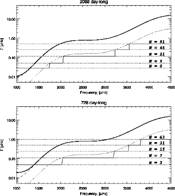
Figure 1: Mode linewidth (long dash) and effective linewidth (solid bold curve), compared to multi-tapers spectral resolution (dotted lines). The optimal number of multi-tapers (see description in text) is indicated by the stepwise solid line, and is such that the spectral resolution remains 5 times smaller than the effective linewidth, whenever possible. Top and bottom panels correspond to 2088-day-long and 768-day-long time series, respectively.

Figure 1 compares the estimate of the mode linewidth to the $N^{\rm th}$ order multi-tapered spectrum resolution, for the pre-selected list of values of $N$, and indicates the number of tapers selected for the fitting.

3.2.3 Detectability Threshold

At low frequencies, the mode amplitude becomes comparable if not smaller than the background noise all the while the mode linewidth becomes smaller than the spectral resolution, forcing the fitting procedure to hunt for small and narrow peaks. This can easily lead to confusing a noise spike with a mode peak and can lead to what is sometimes referred as fitting the grass. To prevent such “grass fitting”, only modes with a power amplitude 3 times greater than the root-mean-squares (RMS) of the residuals to the fit were kept. As the fitting proceeds a sanity check rejects any mode whose amplitude has dropped below that threshold. If this happens, the amplitude of the mode is set to zero and its amplitude and frequency are no longer fitted, leaving the fitting procedure to only adjust the background term to the noise.

As a result of the line of sight apodization of any radial velocity observation, the near sectoral modes ($m\approx\pm\ell$) emerge above the noise background before the near zonal ones ($m\approx 0$). By not using a polynomial expansion in $m$, I end up fitting only the azimuthal degrees that are large enough, and I avoid any potential bias in the estimate of the frequency splittings based on an expansion that would be unevenly constrained.

3.2.4 Fitting Procedure & Initial values

At each iteration the fitting is done in steps, i.e. not all the parameters are adjusted simultaneously right away. The whole procedure is iterated to include progressively better and better estimates of the mode contamination.

An initial value of all the mode parameters is first needed. The initial guess for the mode frequency was computed by using previous estimates of the singlet frequencies ($\nu_{\ell,m}$) and of the polynomial expansion coefficients for the frequency splittings. The frequency table was extended at low frequencies by looking at “derotated” $m$-averaged spectra while the frequency splittings table was extended with values that produced nearly “straight” derotated $m$-averaged spectra. The initial values for the linewidth and the asymmetry were computed from a polynomial parameterization in term of frequency, also based on previous estimates, and extrapolated when needed. The initial amplitude and background parameters were computed from averaging appropriate portions of the section of the spectrum being fitted and then performing a polynomial fit of these values as a function of $m$ with a 3$\sigma$ rejection of outliers.

To make sure that the result is not biased by the initial guess of the parameters, the fitting steps at the very first iteration were different from the ones taken during the consecutive iterations. The first iteration included additional steps where the fitting was done on individual spectra (i.e., one $m$ at a time) instead of the simultaneous fitting of all the $m$.

A sanity check is performed after each step to remove from the fitting any peak with too low of an amplitude. The amplitude of such peaks are set to zero and their amplitude and frequency is no longer fitted. This check is followed by a readjustment of the fitting interval by using for the center of the interval smoothed values resulting from a polynomial fit of the frequencies as a function of $m$, with a 3$\sigma$ rejection of outliers.

3.2.5 Leakage Coefficients

The first leakage coefficients I used for the MDI observations were based on the direct computation of the spatial leakage from the leakage equations (see Section 3.1 of Korzennik, Rabello-Soares, & Schou (2004)). Such calculation leads to an approximation of the actual leakage coefficients as it remains oversimplified by ignoring effects like the detector finite pixel size and the on-board Gaussian weighting performed on the MDI Structure Program images.

A more sophisticated leakage matrices computation was carried out by Schou (1999), by constructing simulated images corresponding to the line-of-sight contribution of each component of a single spherical harmonic mode. These images were then decomposed into spherical harmonic coefficients using the same numerical decomposition used to process the observations. This approach allows to include the effect of the finite pixel size of the detector and incorporates the above mentioned Gaussian weighting. It also takes into account de facto the effects of both the foreshortening at high lattitudes and the image apodization performed in the spatial decomposition.

In both cases, the horizontal and vertical components were computed and the horizontal to vertical displacement ratio, $\beta$, taken to be the theoretical prediction. Using a simple outer boundary condition, i.e. that the Lagrangian pressure perturbation vanishes ($\delta p=0$), the small amplitude oscillation equations for the adiabatic and non-magnetic case lead to an estimate of the ratio $\beta$, given by:

$$\beta_{n,\ell}=\frac{G\;M_{\odot}\;L}{R_{\odot}^{3}\;\omega^{2}_{n,\ell}}=\frac{\nu_{0,\ell}^{2}}{\nu_{n,\ell}^{2}}$$ (9)

where $G$ is the gravitational constant, $M_{\odot}$ is the solar mass, $R_{\odot}$ is the solar radius, $\omega$ is the cyclic frequency ($\omega=2\pi\nu$) and $L^{2}={\ell(\ell+1)}$.

Leakage matrices were also computed by Schou (private communication, 2004) specifically for the GONG observations. The GONG project has also recently computed leakage matrices (Howe & Hill, private communication, 2004) for the GONG observations, but have only included the vertical component. I have therefore used for the fitting of the GONG data Schou’s complete leakage matrix. In all cases, since the time series are long compared to a year I used leakage matrices computed for $B_{\rm o}=0$.

Figure 2 compares the leakage matrix, for selected values of $\ell$ and $\beta$, resulting from my direct and approximate computation to the values computed explicitly by Schou for the MDI instrument. Figure 3 compares the radial component of the leakage matrix as computed by the GONG project and by Schou, for the GONG observations. The differences seen in Figure 2 should not come as a surprise: the wider leakage seen in the explicit computations is primarly the result of the Gaussian weighting. The RMS of the differences for the radial component of the GONG leakage matrices, as shown in Figure 3, is less than 0.2% above $\ell=4$. The discrepancy at $\ell=1$ is due to the fact that the GONG values includes already the effect of subtracting the image average.

3.2.6 Error Bars Computation

Uncertainties on all the fitted parameters were estimated from the covariance matrix of the problem. This covariance matrix was estimated from the Hessian matrix (Press, Teukolsky, Vetterling, & Flannery, 1992) using numerical estimates of the second derivative of the merit function. The increments appropriate for the estimate of these derivatives were based on the size of the shrunk simplex resulting from the fitting.

4 Results

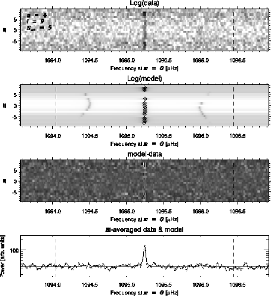
Figure 4: Example of fitting, for MDI 2088-day-long time series, for $\ell=9$, $n=4$ and $N=5$. The top panel shows a fraction of the derotated power spectra (5th sine multi-taper). The second panel from the top shows the model of the power spectra, diamonds indicate the location of the mode frequencies. The third panel from the top shows the residuals and the bottom panel show $m$-averaged profiles (data and model). The vertical dash lines delineates the frequency range used for the fitting. Notice how for this low order case some of the modes amplitudes were not large enough to be fitted.

Figures 4 to 8 illustrate the fitting of the MDI 2088-day-long time series for $\ell=9$ and a selection of values of $n$. It shows that for $n=4$ not all azimuthal orders emerge above the background; it illustrates with $n=7$ the case where modes and leaks are well resolved; it shows for $n=10$ a case where the leaks nearly merge with the main peak; for $n=18$ it illustrates the $n^{\prime}=n+1$, $\ell^{\prime}=\ell-3$ contamination and finally for $n=25$ it presents an example of fitting a high order mode where the optimal spectral estimator uses a large number of multi-tapers.

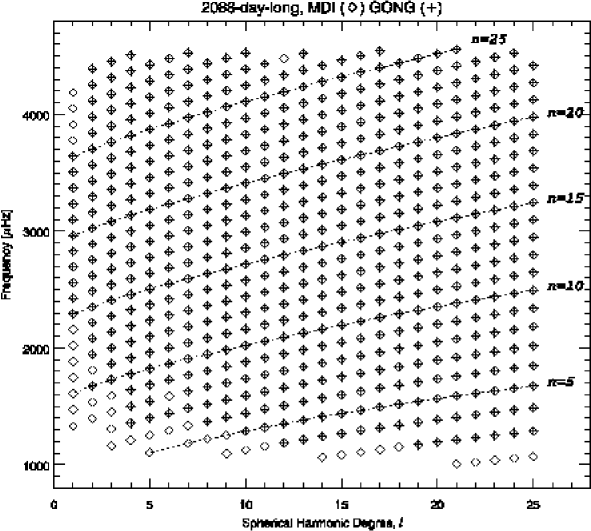
Figure 9: The coverage, in a $\ell-\nu$ diagram, of the fitting range for the 2088-day-long time series, with diamonds for the MDI observations and crosses for the GONG observations. The higher fill factor and lower signal-to-noise ratio of the MDI time series allowed to extend the fitting towards lower frequencies.

I have produced frequency tables of individual multiplets based on MDI and GONG observations for 2088-day-long time series as well as five 728-day-long time series, for $1\leq\ell\leq 25$. The coverage in the $\ell-\nu$ diagram is illustrated in Figure 9 and corresponds to some 15,491 & 14,883 $(n,\ell,m)$ multiplets or some 595 & 554 $(n,\ell)$ singlets for MDI and GONG 2088-day-long time series respectively. The higher fill factor and lower signal-to-noise ratio (SNR) of the MDI time series has allowed me to push the fitting of that time series towards lower frequencies.

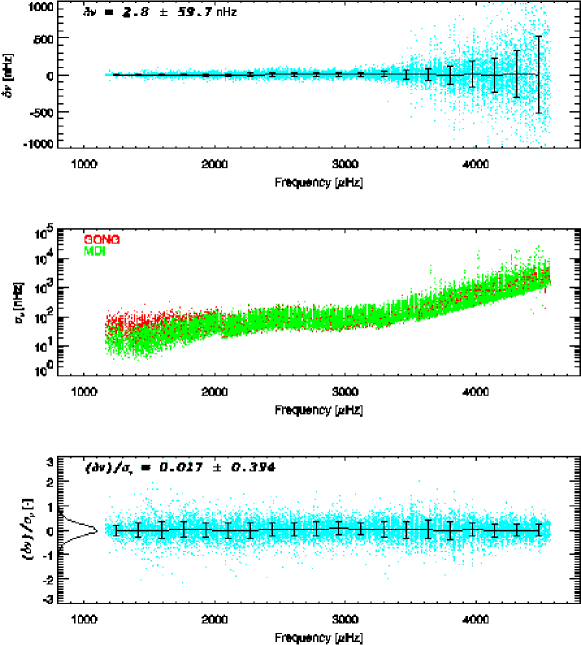
Figure 10: Comparison of fitting results (multiplets) from the two 2088-day-long co-eval MDI and GONG time series. Top panel shows frequency differences while the bottom panel shows the frequency differences scaled to their uncertainties (blue points); in both plots the solid line results from bining the points over 20 equispaced frequency intervals, with the error bars representing the standard deviation within the bin. A histogram of the scaled difference is drawn in the bottom panel. The middle panel shows the frequency uncertainties.

Figure 10 compares the results from fitting the two 2088-day-long co-eval time series, i.e. MDI and GONG. The frequency differences are small ($2.8\pm 59.7$ nHz) and, as expected, increase with frequency – since the accuracy of the fitting decreases as the mode linewidth increases. The reduced frequency differences (${\delta\nu}/{\sigma_{\nu}}$) are uniform and correspond to a nearly Gaussian distribution with a mean of 0.017 and a standard deviation of 0.394. The smaller than expected value of the standard deviation suggests that my estimate of the uncertainties might be too conservative. At low frequency, the error bars on the frequency for the GONG observations are larger than the corresponding one for the MDI observations again as the results of the difference in fill factor and SNR.

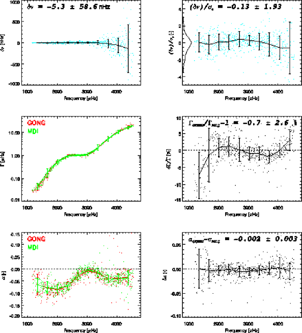
Figure 11: Comparison of fitting results (singlets) from the two 2088-day-long co-eval MDI and GONG time series (top panels). Middle panels compare the mode linewidth ($\Gamma$) while the bottom panels compare the mode asymmetry ($\alpha$). The solid lines correspond to bining individual points (shown as dots) over 10 equispaced frequency intervals, with the error bars representing the standard deviation within the bin.

Figure 11 compares the mode linewidth ($\Gamma_{n,\ell}$) and the asymmetry coefficients ($\alpha_{n,\ell}$), as well as the singlet mode frequencies. The mode singlet was computed by fitting a Clebsch-Gordan polynomial expansion (Ritzwoller & Lavely, 1991) to the multiplets, with a 3$\sigma$ rejection. Mode linewidths and asymmetries between both data sets are nearly identical.

Comparisons for the five 728-day-long segments show similar results, and are quantitatively summarized in Table 2. The larger average frequency difference seen for segment no. 2 results most likely from the data gap at the end of that time series present in the MDI observations. Since the gap is at the end of that time series, the results for MDI and GONG observations do not correspond to the same mean solar activity level.

Table 2: Quantitative Comparison, MDI versus GONG.

	$\delta\nu$		${\delta\nu}/{\sigma_{\nu}}$		${\delta\Gamma}/{\Gamma}$		$\delta\alpha$
	[nHz]				[%]
2088-day-long	$2.8$$\,\pm\,$	$59.7$	$0.017$$\,\pm\,$	$0.394$	$-0.6$$\,\pm\,$	$2.7$	$-0.001$$\,\pm\,$	$0.003$
728-day-long seg. no. 1	$-2.9$$\,\pm\,$	$93.5$	$-0.009$$\,\pm\,$	$0.389$	$1.5$$\,\pm\,$	$3.1$	$0.002$$\,\pm\,$	$0.005$
no. 2	$25.9$$\,\pm\,$	$118.1$	$0.124$$\,\pm\,$	$0.569$	$-1.5$$\,\pm\,$	$3.6$	$-0.002$$\,\pm\,$	$0.003$
no. 3	$-5.7$$\,\pm\,$	$113.4$	$-0.035$$\,\pm\,$	$0.660$	$-1.8$$\,\pm\,$	$1.3$	$-0.001$$\,\pm\,$	$0.003$
no. 4	$2.8$$\,\pm\,$	$85.8$	$0.013$$\,\pm\,$	$0.791$	$0.2$$\,\pm\,$	$1.1$	$-0.002$$\,\pm\,$	$0.004$
no. 5	$5.4$$\,\pm\,$	$100.0$	$0.023$$\,\pm\,$	$0.392$	$-0.1$$\,\pm\,$	$2.0$	$-0.003$$\,\pm\,$	$0.006$

4.1 Comparisons with Previous Estimates

4.1.1 MDI Observations

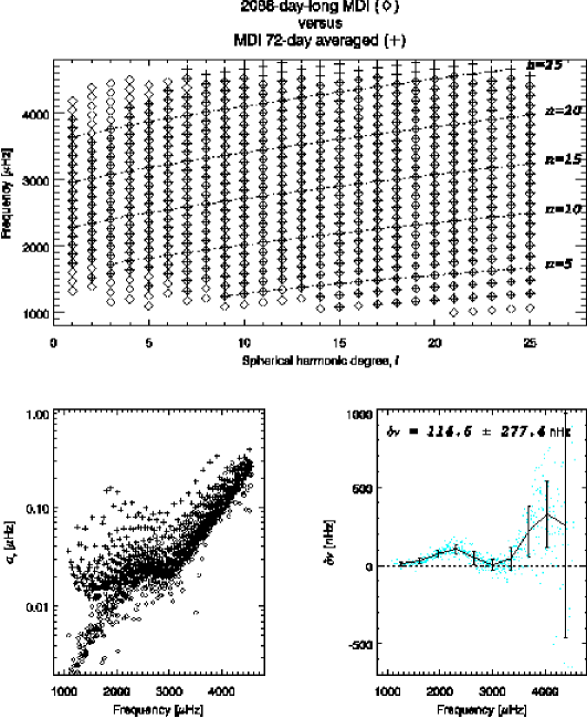
Figure 12: Comparison between singlets resulting from fitting the 2088-day-long MDI time series (diamonds) and the corresponding MDI average values computed from 27 tables resulting from fitting 72-day-long times series. Top panel shows the respective coverage in an $\ell$ – $\nu$ diagram. The lower left panel compares the frequency uncertainties, while the lower right shows the frequency differences (dots) and these differences binned over 10 equispaced frequency bins – the error bars represent the standard deviation inside each bin.

Figure 12 compares results from my fit to the MDI 2088-day-long time series to average values computed from 27 tables resulting from fitting 72-day-long times series that covers the same time span and are routinely computed by the MDI team (Schou, 1999). The averaging was weighted by the uncertainty – to reflect the relative fill factor of each period. The comparison is for singlets, since the MDI fitting procedure uses a polynomial expansion in $m$.

The top panel illustrates the region of the $\ell$ – $\nu$ diagram where fitting a very long time series allows for detecting additional low order modes. The comparison of the resulting fitting uncertainty (lower right) shows – as expected – that at high frequency the uncertainty is dominated by the mode linewidth while at low frequency by the length of the time series.

This figure also shows a systematic difference between frequencies, with a specific frequency dependence. One obvious reason for this difference is the fact that Schou’s fitting uses a symmetric profile while I am fitting an asymmetric one.

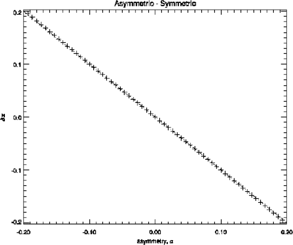
Figure 13: Offset resulting from fitting a symmetric profile to an asymmetric peak, as a function of the asymmetry coefficient, $\alpha$, for a fixed FWHM. The predicted offset (crosses) scales nearly lineary with the asymmetry coefficient (dash line).

To estimate the effect of fitting a symmetric profile to an asymmetric peak I have computed a grid of isolated asymmetric profiles and fitted them with symmetric ones. The resulting offset in frequency varies nearly linearly with the asymmetry coefficient as defined in my parameterization, for a given FWHM, as shown in Figure 13. The systematic error introduced by fitting an asymmetric peak with a symetric profile is thus given by

$$\nu_{\rm asymmetric}-\nu_{\rm symmetric}=-\alpha\,\Gamma/2$$ (10)

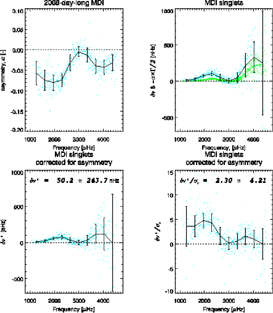
Figure 14: Observed asymmetry (top left) and estimate of systematic frequency offsets due to fitting a symmetric profile to an asymmetric peak (green points in top right panel) compared to observed differences (blue points and solid line in top right panel), for MDI values. The bottom panels show residual differences after correcting for the effect of not including the mode asymmetry. The solid lines represent the values (blue dots) binned over 10 equispaced frequency bins. The standard deviation inside each bin is represented by the error bars.

Roughly half of the frequency differences seen in Figure 12 can be explained by this model, as shown Figure 14. The residual differences after correcting for the asymmetry using Eq. 10, are marginaly significant, i.e. at the 4$\sigma$ level, and still show a systematic trend with frequency.

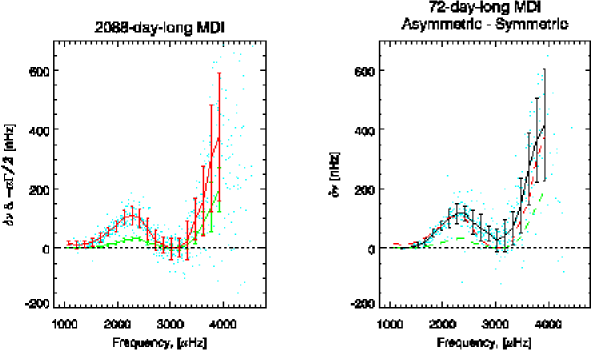
Figure 15: (Left) Comparison of observed differences between fitting the 2088-day-long MDI time series and the corresponding MDI average values computed from 27 tables resulting from fitting 72-day-long times series (raw values as blue dots and binned values shown as the red line) with the predicted differences resulting from a simple model (green points and line) of fitting an isolated symmetric profile to an asymmetric one. (Right) Frequency differences resulting from symmetric and asymmteric fits carried out by Schou using a 72-day-long MDI time series (individual values shown as dots, solid line represents binned values) compared to the frequency differences shown in the left panel (red line, binned values) and the simple model prediction (green line, binned values).

Back in 1991, Schou (private communication) fitted one 72-day-long MDI time series using an asymmetric profile as well as a symmetric one. The comparison between his symmetric and asymmetric fitting for that time series and for modes up to $\ell=25$ is shown in Figure 15. The frequency differences compare very well with the systematic differences seen in Figure 12 and are nearly twice as large as the values predicted by Eq. 10. While one could be tempted to rescale the prediction of Eq. 10 by some ad hoc factor, I must point out that not only there is no rationale for this – unless either the leakage matrix or the horizontal to vertical ratio or both are substantially wrong – but also that a single factor would not match the observed differences (such factor would have to be quite different for frequencies above and below 3 mHz).

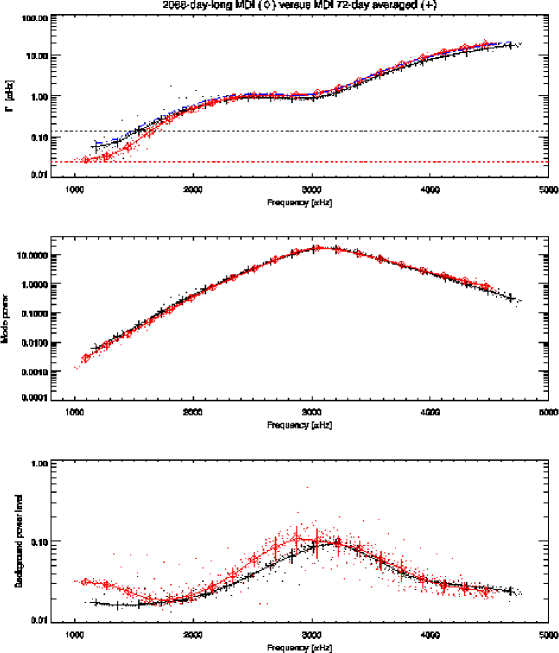
Figure 16: Comparison between results from fitting the 2088-day-long MDI time series (red dots & diamonds) and the corresponding MDI average values computed from 27 tables resulting from fitting 72-day-long times series (black dots & crosses). The top panel compares linewidths, the horizontal lines correspond to the respective time series frequency resolution, while the blue curve illustrates the factor 1.2 between the two sets. The middle panel compares the mode power ($A\times\Gamma$). The bottom panel compares the background power level.

Comparison of mode linewidths, amplitudes and background levels are shown in Figure 16. The mode linewidth comparison shows a small systematic discrepancy (i.e., a factor of 1.2) above 2.5 mHz, while below 2.5 mHz it indicates that the MDI estimates are too large – most likely as a result of the resolution limit of the 72-day-long time series – despite being corrected for the intrinsic frequency resolution of the time series. The mode power and background level estimates compare rather well.

4.1.2 GONG Observations

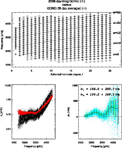
Figure 17: Comparison between results from fitting the 2088-day-long GONG time series (diamonds or black dots) and the corresponding GONG average values computed from 58 tables resulting from fitting 36-day-long times series (crosses or red dots). Top panel shows the respective coverage in an $\ell$ – $\nu$ diagram, when computing averages only if the multiplet is present in at least 10 of the 58 tables. The lower left panel compares the frequency uncertainties for the multiplets, while the lower right panel shows the frequency differences (dots, multiplets) and the differences (singlets and multiplets) binned over equispaced frequency bins – the error bars represent the standard deviation inside each bin. The binned singlets differences is shown as the green curve.

Figure 17 compares results from my fit to the GONG 2088-day-long time series to average values based on 58 tables resulting from fitting 36-day-long times series that covers the same time span and are routinely computed by the GONG project (Hill et al., 1996). The averaging was weighted by the uncertainty – to reflect the relative fill factor of each period. Singlets were then computed – by fitting a Clebsch-Gordan polynomial expansion to the multiplets, with a 3$\sigma$ rejection of outliers – to produce comparisons similar to the case of the MDI observations.

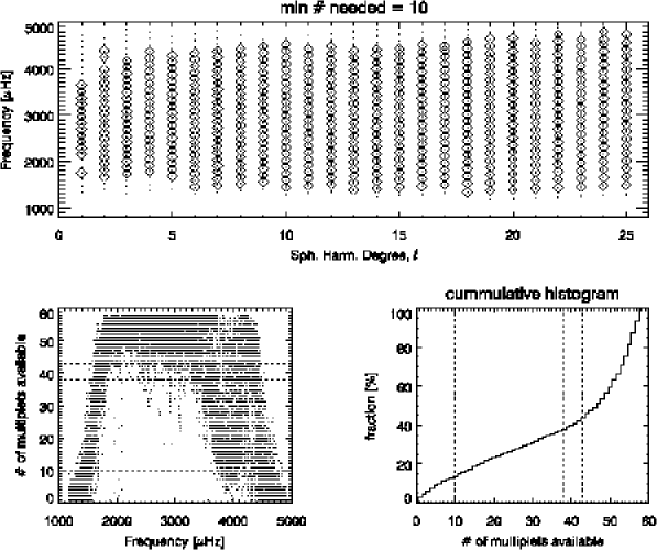
Figure 18: This figure illustrates a consistency problem present in the GONG frequency tables. The top panel shows in an $\ell$–$\nu$ diagram averaged multiplets (dots) and the resulting average singlets when only considering multiplets that are present in at least 10 of the 58 tables. The lower left panel shows the number of times each multiplet is present – as a function of its frequency. The lower right panel shows the cumulative histogram of the number of times a multiplet is present. Dashed lines are draw at 10 (the value I ended up using) and at 2/3 and 3/4 of 58. When using 10 as a threshold only some 15% of the mode set has to be dropped, while if I would use a more conservative threshold nearly half of the mode set would be ignored. Note also how using only such a threshold can skew singlet estimates at the edge of the covered $\ell$–$\nu$ diagram.

Unfortunately the GONG fitting methodology does not produce consistent frequency tables: for a substantial number of modes the same multiplets are not fitted every time, as illustrated in Figure 18. The averages used in the comparison in Figure 17 correspond to the case where the multiplet is measured at least 10 times out of 58. Using a higher threshold – to obtain better temporal averages – would reduce substantially the resulting frequency set.

The lower SNR of the GONG observations at low frequency does not allow to push mode fitting down to orders as low as for the MDI observations. But using a long time series still allowed me to fit low order modes that are rarely (less than 10 out of 58 times) fitted by the GONG project.

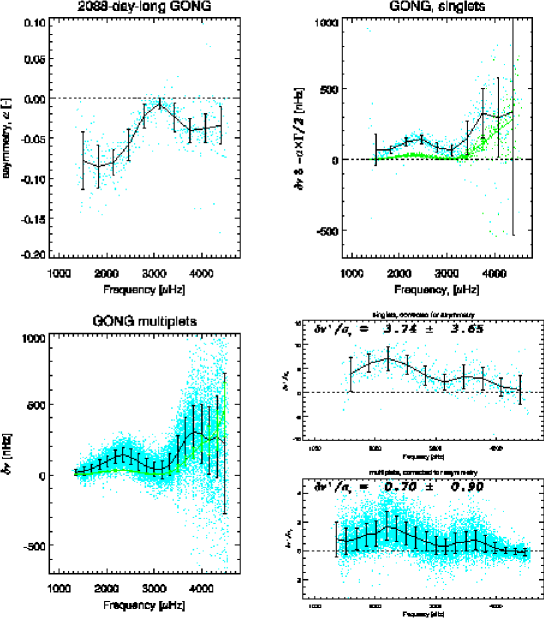
Figure 19: Observed asymmetry (top left) and estimate of systematic frequency offsets due to fitting a symmetric profile to an asymmetric peak (in green, top right) compared to observed differences (blue dots and solid line) for GONG singlets. The bottom left panel compares directly the multiplets (blue dots and solid line) to the estimate of systematic offsets (green curve). The bottom right panels show the reduced frequency differences, after correcting for the effect of not including the mode asymmetry, for singlets and multiplets.

The frequency comparison, presented in Figure 19, shows systematic differences – whether using singlets or multiplets. The GONG project also fits a symmetric profile, hence some of the discrepency can be attributed to fitting a symmetric profile to an asymmetric peak. The residual differences, after correcting for the asymmetry using Eq. 10, are also shown in Fig. 19 for both singlets and multiplets. The corrected singlets show marginally significant differences (at the 4$\sigma$ level) with a systematic trend with frequency as for the MDI comparison (see Fig. 14). The corrected multiplets show the same trend with frequency, but with less significance (0.8$\sigma$) simply because the uncertainties on the multiplets are larger.

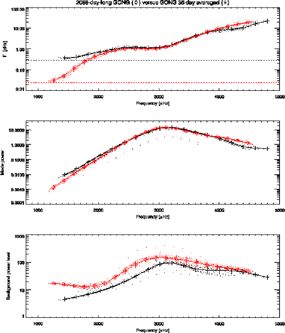
Figure 20: Comparison between results from fitting the 2088-day-long GONG time series (red dots & diamonds) and the corresponding GONG average values computed from 58 tables resulting from fitting 36-day-long times series (black dots & crosses). The top panel compares linewidths, the horizontal lines correspond to the respective time series frequency resolution. The middle panel compares the mode power ($A\times\Gamma$). The bottom panel compares the background power level.

Comparison of mode linewidth, presented in Figure 20, indicates that below 2.5 mHz the GONG values are dominated by the frequency resolution of the time series – not surprisingly, since by contrast to MDI’s estimates they are not corrected for that effect – while agreeing rather well above 2.5 mHz – except for the dip between 4 and 4.5 mHz. Mode power levels compare rather well – except at low and high frequencies – while estimates of the background level do not compare as well.

4.1.3 MDI Observations - II

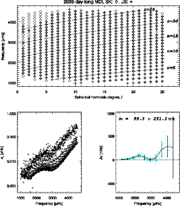
Figure 21: Comparison of MDI singlets resulting from this work (crosses) and from Schou’s fitting to the same 2088-day-long time series (diamonds). Coverage in the $\ell$ – $\nu$ diagram is very similar. My estimate of frequency uncertainties appears too conservative while the frequency differences show a systematic pattern with frequency.

Schou (private communication, 2004) has carried out a fitting of the 2088-day-long time series as well – using the same methodology he uses for fitting the 72-day-long time series. He has graciously provided me with the results of that fit for a direct comparison that is shown in Figures 21 and 22. Coverage over the $\ell-\nu$ diagram is comparable, while the comparison of the uncertainties on the frequency suggests – as indicated earlier – that my estimates might be too conservative, by as much as a factor 3. The comparison of the mode frequencies (singlets) shows again systematic differences, that are in part explained by the effect of not including the mode asymmetry.

The residual frequency differences after correcting for the asymmetry using Eq. 10 are at the 3$\sigma$ level and present a residual systematic variation with frequency. The mode linewidths agree remarkably well (the discrepancy factor of $1.2$ is no longer present) – except at very low frequency where my uncorrected estimates are biased by the frequency resolution. The mode power and background level estimates compare rather well.

4.2 Changes with Epoch

4.2.1 MDI & GONG Observations

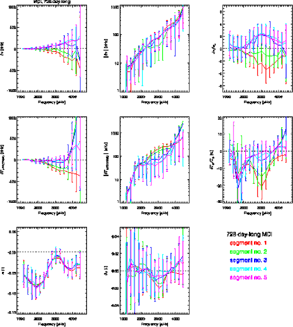
Figure 23: Changes in singlet parameters, with respect to the values estimated from the 2088-day-long time series, using MDI observations over the five 728-day-long segments. Panels in the top row show change in frequency, panels in the middle row show changes in linewidth, while the panels in the bottom row compare estimates of asymmetry. Binned values, over equispaced interval in frequency are shown, with the standard deviation within the bin indicated by the error bars.

Changes in frequency, linewidth and asymmetry, with respect to the values estimated from the 2088-day-long time series, and using MDI observations over the five 728-day-long segments are illustrated in Figure 23. This figure shows that the frequency changes with epoch scale with frequency and range from 5 to 800 nHz, a now well established property that can be explained by changes with activity levels concentrated near the solar surface. The frequency changes at low degrees and very low frequency are very small and barely significant. These changes are thus small enough to justify using very long time series to fit these modes.

Changes in linewidth with epoch also scale with frequency, with relative changes as large as 20% observed around 3 mHz. Changes at low frequency are hard to measure since the measured width is dominated by the spectral resolution. The mode asymmetry shows no significant sign of change with time.

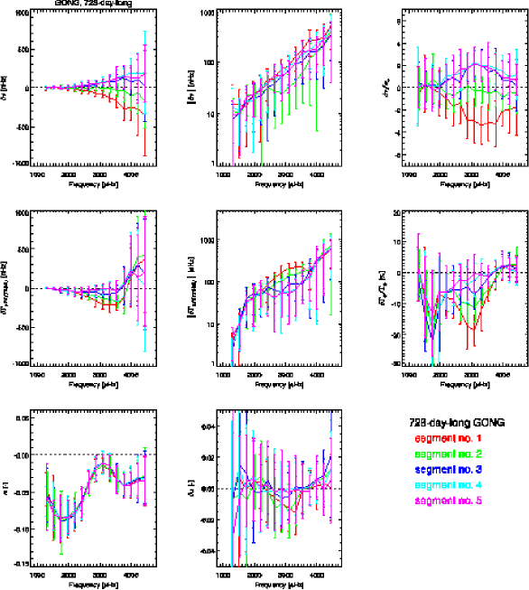
Figure 24: Changes in singlet parameters, with respect to the values estimated from the 2088-day-long time series, using GONG observations over the five 728-day-long segments. Panels in the top row show change in frequency, panels in the middle row show changes in linewidth, while the panels in the bottom row compare estimates of asymmetry. Binned values, over equispaced interval in frequency are shown, with the standard deviation within the bin indicated by the error bars.

Changes in frequency, linewidth and asymmetry, with respect to the values estimated from the 2088-day-long time series, and using GONG observations over the five 728-day-long segments are shown in Figure 24. These are very similar to the ones for the MDI data.

4.2.2 Changes as a Function of Frequency and Azimuthal Order

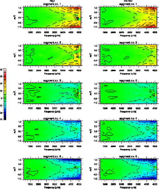
Figure 25: Changes in frequency for each 728-day-long segment with respect to the values estimated from the 2088-day-long time series based on multiplets and plotted as a function of frequency and the ratio $m/\ell$, for MDI (left column) and GONG (right column). The frequency differences were binned over a grid equispaced in $\nu$ and $m/\ell$.

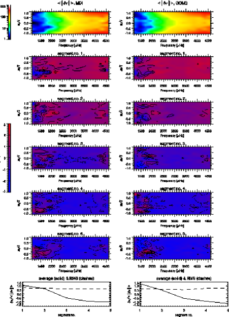
Figure 26: Top panels: average of the absolute value of the changes in frequency for each 728-day-long segment with respect to the values estimated from the 2088-day-long time series, as shown in Fig. 25. Middle 5 panels: frequency changes divided by the average of the absolute values, for each 728-day-long segment. Bottom panels: average and RMS of the changes scaled by the average of the absolute values as a function of segment number. The RMS remains nearly constant while the average varies with time, indicating that the changes in frequencies can be described by a fixed pattern nearly constant in time scaled by a time dependant factor.

Changes in frequency, computed from multiplets rather than singlets, with respect to epoch are shown for both data set in Figure 25, as a function of frequency and azimuthal order. The individual frequency differences were binned over an equispaced grid in $\nu$ and $m/\ell$ to generate this figure. This figure shows that the change in frequencies is concentrated near the sectoral modes and that it is dominated by a pattern mostly symmetric in $m$ and nearly constant in time – given a time dependant scaling factor. This is clearly illustrated in Figure 26 where the top panels show the average of the absolute value of the binned frequency differences, while the midle panels show how well the changes for each segment scale with that average. The bottom panels show the variation of the mean scaled changes and the nearly constancy of the RMS of these scaled changes.

5 Conclusions

Fitting very-long time series has allowed me to push the precise characterization of low degree modes to lower frequencies. The use of such a very long time series is well justified for fitting of these modes since their variation with activity remains small and comparable to the fitting uncertainty itself. The resulting table of frequencies will allow us to further improve inferences on the structure and dynamics of the solar deep interior.

The methodology I have developed includes the most up-to-date procedural elements: the use of an optimized sine multi-tapered power spectrum estimator; the simultaneous fitting of all azimuthal orders – each individually parameterized; the use of the complete leakage matrix and the inclusion of an asymmetric mode profile.

The inter-comparison of the values resulting from my fit to the co-eval MDI and GONG time series is very good. The comparison with equivalent values produced by the MDI team and the GONG project is not as good. It is complicated by the inclusion in my fit of the mode profile asymmetry. The observed differences in mode frequencies are most likely dominated by the effect of including or not the mode profile asymmetry. Unfortunately a simple model for this effect does not fully account for the discrepancies.

Figure 2: Comparison of leakage matrix, for selected values of $\ell$ and $\beta$, resulting from a direct computation (analytical approximation) to the values computed explicitly by Schou for the MDI instrument. The RMS of the differences is around 4 to 7% below $\ell=10$ and less than 2% above. The “wider” leakage seen in the explicit computation is primarly the result of including the Gaussian weighting of the MDI images for the Structure Program data.

Figure 3: Comparison of the radial component of the leakage matrix computed for the GONG observations by the GONG project (black) and by Schou (red). The RMS of the differences is less than 0.2% above $\ell=4$.

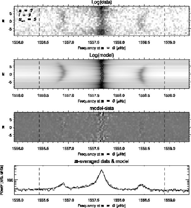
Figure 5: Example of fitting, as in Figure 4, but for $n=7$. In this case the mode and the leaks are still well resolved and all the modes are well above the background.

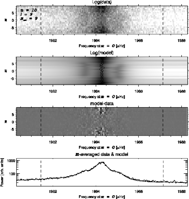
Figure 6: Example of fitting, as in Figure 4, but for $n=10$. In this case the closest spatial leaks ($\delta m=\pm 2$, $\delta\ell=0$) are barely resolved, and blends with the main peak in the $m$-averaged spectrum.

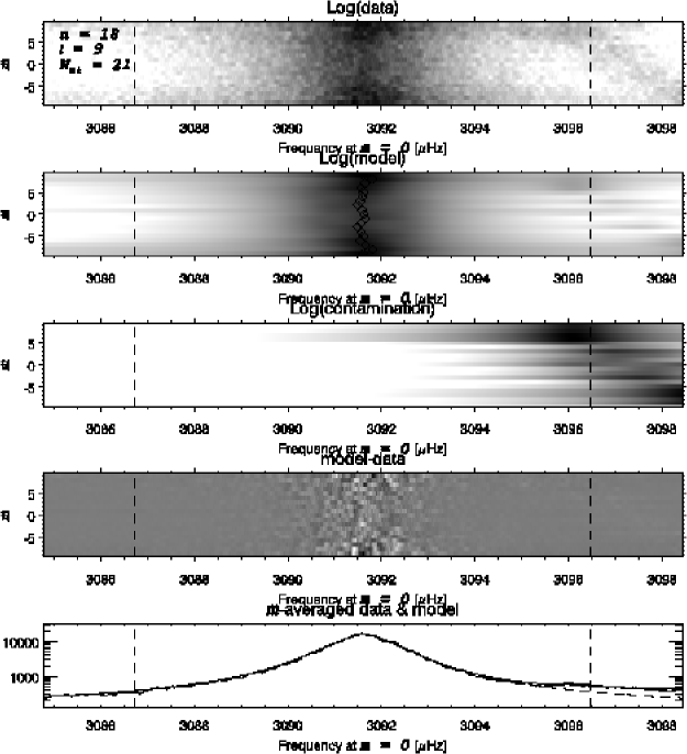
Figure 7: Example of fitting, as in Figure 4, but for $n=18$, to illustrate the $n^{\prime}=n\pm 1$, $\ell^{\prime}=\ell\mp 3$ contamination. The contamination – illustrated by itself in an additional panel – is in this case relatively well separated from the main peak. The $m$-averaged model without including this contamination is illustrated in the bottom panel by the dashed line.

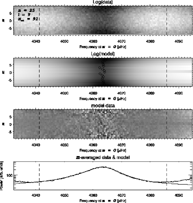
Figure 8: Example of fitting, as in Figure 4, but for $n=25$, where the mode linewidth is very large and a large number of tapers has been used to estimate the power spectrum ($N=91$).

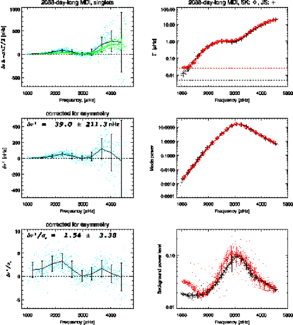
Figure 22: Comparison of MDI singlets resulting from this work (crosses) and from Schou’s fitting to the same 2088-day-long time series (diamonds). The frequency differences (blue dots and black curves for binned values) are not fully explained by the effect of not including an asymmetry in the mode fitting (green points, top left panel). Residual differences, after correcting for the effect of not including the mode asymmetry, remain at the 3$\sigma$ level. Mode linewidth and power as well as estimates of background level compares remarkably well.

References

- Anderson, Duvall, & Jefferies (1990) Anderson, E. R., Duvall, T. L., & Jefferies, S. M. 1990, ApJ, 364, 699
- Appourchaux, Rabello-Soares, & Gizon (1998) Appourchaux, T., Rabello-Soares, M.-C., & Gizon, L. 1998, A&AS, 132, 121
- Duvall et al. (1993) Duvall, T. L., Jefferies, S. M., Harvey, J. W., Osaki, Y., & Pomerantz, M. A. 1993, ApJ, 410, 829
- Hill et al. (1996) Hill, F., et al. 1996, Science, 272, 1292
- Jimenez-Reyes (2001) Jimenez-Reyes, S. 2001, Ph.D. Thesis, La Laguna Univ.
- Korzennik (1990) Korzennik, S. G. 1990, Ph.D. Thesis, UCLA.
- Korzennik, Rabello-Soares, & Schou (2004) Korzennik, S. G., Rabello-Soares, M. C., & Schou, J. 2004, ApJ, 602, 481
- Libbrecht (1988) Libbrecht, K. G. 1988, ApJ, 334, 510
- Nelder & Mead (1965) Nelder, J.A., Mead, R. 1965, Computer Journal, 7, 308.
- Nigam & Kosovichev (1998) Nigam, R. & Kosovichev, A. G. 1998, ApJ, 505, L51
- Press, Teukolsky, Vetterling, & Flannery (1992) Press, W. H., Teukolsky, S. A., Vetterling, W. T., & Flannery, B. P. 1992, Cambridge: University Press, —c1992, 2nd ed.,
- Rabello-Soares & Appourchaux (1999) Rabello-Soares, M. C. & Appourchaux, T. 1999, A&A, 345, 1027
- Ritzwoller & Lavely (1991) Ritzwoller, M. H. & Lavely, E. M. 1991, ApJ, 369, 557
- Schou (1992) Schou, J. 1992,Ph.D. Thesis, Aarhus Univ.
- Schou (1999) Schou, J. 1999, ApJ, 523, L181
- Thiery (2000) Thiery, S. 2000, Ph.D. Thesis, Paris XI Univ.
- Toutain et al. (1998) Toutain, T., Appourchaux, T., Fröhlich, C., Kosovichev, A. G., Nigam, R., & Scherrer, P. H. 1998, ApJ, 506, L147