The Structure of the Local Interstellar Medium. III. Temperature and Turbulence

Abstract

We present 50 individual measurements of the gas temperature and turbulent velocity in the local interstellar medium (LISM) within 100 pc. By comparing the absorption line widths of many ions with different atomic masses, we can satisfactorily discriminate between the two dominant broadening mechanisms, thermal broadening, and macroscopic nonthermal, or turbulent, broadening. We find that the successful use of this technique requires a measurement of a light ion, such as D I, and an ion at least as heavy as Mg II. However, observations of more lines provides an important consistency check and can also improve the precision and accuracy of the measurement. Temperature and turbulent velocity measurements are vital to understanding the physical properties of the gas in our local environment, and can provide insight into the three-dimensional morphological structure of the LISM. The weighted mean gas temperature in the LISM warm clouds is 6680 K and the dispersion about the mean is 1490 K. The weighted mean turbulent velocity is 2.24 km s^-1 and the dispersion about the mean is 1.03 km s^-1. The ratio of the mean thermal pressure to the mean turbulent pressure is $P_{\rm T}/P_{\xi}\,\sim\,26$. Turbulent pressure in LISM clouds cannot explain the difference in the apparent pressure imbalance between warm LISM clouds and the surrounding hot gas of the Local Bubble. Pressure equilibrium among the warm clouds may be the source of a moderately negative correlation between temperature and turbulent velocity in these clouds. However, significant variations in temperature and turbulent velocity are observed. The turbulent motions in the warm partially ionized clouds of the LISM are definitely subsonic, and the weighted mean turbulent Mach number for clouds in the LISM is 0.19 with a dispersion of 0.11. These measurements provide important constraints on models of the evolution and origin of warm partially ionized clouds in our local environment.

1 Introduction

Understanding the physical state of the interstellar medium (ISM) is a fundamental area of research in astrophysics. Theoretical studies of the phases of the ISM have produced classic papers in the astrophysical literature (e.g., Field, Goldsmith, & Habing, 1969; McKee & Ostriker, 1977), the details of which are still being discussed, analyzed, and refined to this day (Cox, 1995; Wolfire et al., 1995a, b; Heiles, 2001a). These classical theoretical models predict the stable coexistence in pressure equilibrium of various phases of interstellar matter: the cold neutral medium (CNM), the warm neutral medium (WNM), the warm ionized medium (WIM), and the hot ionized medium (HIM). Detailed observations are required to test the theory and provide direction for future modifications.

The heliosphere is surrounded by warm partially ionized material (Redfield & Linsky, 2000) in the local interstellar medium (LISM), which has properties intermediate between those of the WNM and WIM theoretical models. The LISM is embedded in a larger cavity, the Local Bubble, presumably filled with hot rarefied gas. Very little cold material, or CNM, resides in the LISM, as is shown by the lack of Na I absorption towards nearby targets (Lallement et al., 2003; Sfeir et al., 1999; Welty, Morton, & Hobbs, 1996; Welsh et al., 1994). However, observations of this cold material are made from low ionization absorption line measurements (Jenkins & Tripp, 2001), and from absorption and emission in the 21 cm hyperfine structure line of H I (Heiles, 2001b). The HIM that presumably pervades the Local Bubble, was identified by the presence of soft X-ray emission by Snowden et al. (1998). The Cosmic Hot Interstellar Plasma Spectrometer (CHIPS) instrument, which was launched on 2003 January 12, should provide important new observations of this rarefied gas (Hurwitz & Sholl, 1999).

Observations of the warm partially ionized gas are vital to unlocking the physical structure of the ISM. Distant WNM environments can be probed by analysis of the 21 cm hyperfine structure line of H I, where the WNM is detected in emission and the CNM in absorption. However, only upper limits of the temperature can be inferred because the contribution of nonthermal, or turbulent, broadening cannot be measured separately (Heiles, 2001b). Ultraviolet (UV) spectra of absorption lines can be used to make accurate temperature and turbulent velocity measurements of gas in the LISM by comparing the observed line widths of ions with different atomic masses. However, for distant lines of sight, the absorption features are typically severely blended, and most information regarding the influences of thermal and turbulent broadening mechanisms on the line widths is lost. Only crude estimates of the temperature can be made from the detection or nondetection of various ionization stages of observed elements (Welty et al., 2002). Therefore, nearby targets, and the intervening warm partially ionized gas, represent a unique opportunity to analyze unsaturated absorption lines with simple and well-characterized component structures so as to measure accurately the temperature and turbulence along lines of sight to these targets.

After more than a decade of high resolution UV spectroscopy with the Hubble Space Telescope (HST), we are beginning to accumulate a critical number of observations of the LISM. Collections of observations presented by Redfield & Linsky (2002, 2004), and researchers referenced therein, provide an opportunity to make fundamental physical measurements of the velocity, temperature, and turbulent velocity in the gas along the line of sight. Researchers investigating the LISM absorption lines towards nearby stars typically calculate a temperature and turbulent velocity for a given line of sight, but do not analyze the results in the context of the LISM as a whole. We present here the first systematic survey of temperature and turbulent velocity measurements for the LISM gas within 100 pc of the Sun.

2 Calculating the Temperature and Turbulent Velocity

By measuring the LISM absorption line widths of many ions, one can disentangle the contributions of thermal and turbulent broadening. The standard equation that relates the absorption line width, or Doppler parameter ($b$), and the temperature ($T$) and turbulent velocity ($\xi$) of the absorbing gas is

$$b^{2}=\frac{2kT}{m}+\xi^{2}=0.016629\frac{T}{A}+\xi^{2},$$ (1)

where $k$ is Boltzmann’s constant, $m$ is the mass of the ion, and $A$ is the atomic weight of the ion in atomic mass units. Although only two line width measurements are required to solve Equation 1 for the temperature and turbulence, an accurate solution requires that the two ions have very different masses. Ideally, one would like to compare line widths of the two ions with the greatest mass differences that are observed in the LISM, hydrogen and iron. Iron is an excellent candidate because there are a number of resonance lines in the 2000-2600 Å region that span a range of optical depths, permitting precise measurements of unsaturated absorption lines. In addition, due to its large mass, thermal broadening is typically negligible and the line is intrinsically narrow, which improves the precision of the line fitting and facilitates the identification of individual velocity components. Redfield & Linsky (2002) presented an inventory of all measured Fe II LISM absorption line measurements toward stars within 100 pc.

The light ions, however, pose more of a problem. Although the strong Ly-$\alpha$ line at 1215 Å is available for measuring the H I absorption line width, the line is heavily saturated and very broad, which makes estimating the stellar continuum difficult. This line can also be broadened by heliospheric and astrospheric absorption components (e.g., Linsky & Wood, 1996; Wood, Linsky, & Zank, 2000). Deuterium is the next lightest ion, only twice as heavy as hydrogen. The D I absorption line is offset by roughly $-82\,$km s^-1 from the H I Ly-$\alpha$ line. For short lines of sight the D I line is typically unsaturated. Since the D I line usually lies on the extended wing of the broad stellar Ly-$\alpha$ emission line, it is relatively straightforward to interpolate the background continuum. D I is the subject of many papers and has been analyzed by many groups. Redfield & Linsky (2004) bring together the full collection of D I Ly-$\alpha$ observations towards stars within 100 pc with known velocity component structures, including many new measurements.

In Figures 1a through 1m, we present our measurements of the temperature and turbulent velocity for all 50 observed LISM components along 29 lines of sight to stars located within 100 pc that have absorption line width measurements of D I and an ion at least as heavy as Mg II. Sources for all of the Doppler width measurements used in Figures 1a-1m can be found in Redfield & Linsky (2002) and Redfield & Linsky (2004). For each velocity component along a particular sightline, there are two plots to visualize the temperature and turbulent velocity measurement. On the left side is a color coded plot of temperature versus turbulent velocity. For a given measured Doppler parameter of a particular ion, Equation 1 defines a curve in the temperature-turbulent velocity plane. The accompanying pair of dashed lines indicate the $\pm\,1\sigma$ error bars around the best fit curve (solid line). The black “$\times$” symbol denotes the best fit value of the temperature and turbulent velocity based on the widths of the deuterium line and all other line widths measured from high resolution echelle (STIS E140H and E230H and GHRS Ech-A and Ech-B) spectra. The surrounding black contours enclose the 1$\sigma$ and 2$\sigma$ ranges for both values. The $1\sigma$ and 2$\sigma$ error contours were determined by calculating the $\Delta\chi$ appropriate for the 68.27% and 95.45% confidence level, respectively, as described in Bevington & Robinson (1992). Except for deuterium, all the other absorption lines are not fully resolved at moderate resolution. Therefore, systematic errors, such as, inaccurate instrumental line spread functions, unresolved blends, and saturated lines, can potentially dominate the moderate resolution results. For this reason, the fits were made only to the deuterium measurement and all additional high resolution measurements. The moderate resolution data are plotted as consistency checks. Two sightlines, HR 1099 and $\beta$ Cet, analyzed by Piskunov et al. (1997), use the H I Doppler width as opposed to D I. Although they did not provide an independent D I line width measurement, their H I Doppler width was forced to agree with the D I line. Therefore, despite the difficulty of analyzing the H I absorption line, these are likely to be reasonable estimates of the H I Doppler parameter.

The plots on the right show another visualization for determining the temperature and turbulent velocity. Here, the observed Doppler parameter for each ion is plotted versus its atomic mass. The red and blue symbols represent the observations that were taken with high resolution and moderate resolution, respectively. The solid line indicates the best fit curve for the temperature and turbulence, as defined by Equation 1. The shaded region encompasses all fits within the $1\sigma$ contour shown in the plot on the left.

Both plots clearly demonstrate the need for using both the light ion, deuterium, and preferably the heaviest ion, iron, for calculating the temperature and turbulent velocity. The deuterium curve in the plots on the left is nearly vertical, whereas the curve for iron is practically horizontal, indicating that for deuterium thermal broadening dominates, and the line width is relatively insensitive to turbulent broadening. The reverse is true for iron. In the plots on the right, D I lies on the steep part of the curve, while practically all the remaining ions are on the flat part of the curve, where turbulent broadening dominates, and the line widths are independent of atomic mass and thermal broadening. Deuterium is significantly broader than all of the other ions and is the only serious constraint on the temperature of the gas. Even the next lightest ion observed in the LISM, C II, is already 6 times the mass of deuterium, and predominantly horizontal in the plots on the left and on the flat part of the curve in the plots on the right.

Although only two measurements are required to solve Equation 1, the intermediate mass ions provide important consistency checks against potentially unidentified systematic errors in the heavy and light ion measurements. Often, the lines of C II and O I have large errors in the Doppler parameter measurement because they are highly saturated. HZ 43 in Figure 1j provides an excellent example of agreement among all of the measured ions. Only a handful of components show significant disagreement among the observed ions. In particular, Altair (Figures 1c and 1d) shows possible discrepancies in the observed C II Doppler width. This is most likely due to the C II absorption line being highly saturated. Low signal-to-noise observations or multiple closely spaced components can also make a precise Doppler width measurement difficult. Otherwise, this technique offers a unique opportunity to measure accurately the temperature and turbulent velocity in distinct collections of gas in the LISM.

Table 1 lists the best fit temperature and turbulent velocity for all components shown in Figures 1a through 1m. The $\pm\,1\sigma$ error bars were determined by fixing each parameter in turn, and calculating the $\Delta\chi$ appropriate for the 68.27% confidence level, as described in Bevington & Robinson (1992). To determine the best fit temperatures and turbulent velocities for each velocity component, we weighted the observed Doppler parameters inversely to their measurement errors. We also include, for each component, the list of ions for which a Doppler width was included in the fit. Two is the minimum number of ions required for this technique, but our fits typically include Doppler widths from $\sim$ 5 different ions, and in some cases as many as eight. Also included in Table 1, are the galactic coordinates and distance to the background star, and the weighted mean velocity measurements for the observed LISM absorption components.

3 Temperature and Turbulent Velocity Distribution in the LISM

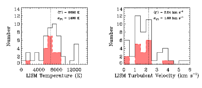
Figure 2: Distributions of measured temperatures and turbulent velocities in the LISM for clouds within 100 pc. The temperature distribution is peaked at the canonical LISM temperature $\sim$ 7000 K. The weighted mean of our sample is $\langle\,T^{\prime}\,\rangle\,=\,$6680 K, while the dispersion about the mean is 1490 K. The weighted mean of the turbulent velocity distribution is $\langle\,\xi^{\prime}\,\rangle\,=\,$2.24 km s^-1, with a dispersion about the mean of 1.03 km s^-1. The weighted mean is indicated by a dotted line. The shaded subsamples represent our most precise measurements, defined by their absolute error being less than the standard deviation of the entire sample.

The distributions of temperatures and turbulent velocities in the LISM are shown in Figure 2. The temperature distribution is strongly peaked, although significant outliers exist and range from 0 K up to 12900 K. In particular, 18% of the sample, or between 8% and 38% if we include the 1$\sigma$ error bars, include measured cloud temperatures that are $<\,5000$ K, which is in the thermally unstable regime (McKee & Ostriker, 1977). Heiles (2001b) discussed a survey that is currently obtaining Zeeman splitting observations of H I 21 cm ISM absorption lines that may be able to provide a distribution of temperatures for more distant warm ISM environments. Our turbulent velocity distribution is likewise peaked, and the range of values extends from 0 km s^-1 to 5.6 km s^-1. The few very high turbulent velocity measurements are likely caused by unresolved blends. Because line widths can increase greatly when there are unresolved closely-spaced velocity components, which are common in the LISM (cf. Welty, Morton, & Hobbs, 1996), undetected blends will increase the widths of all observed ions, although only by a small amount for deuterium. Therefore, the gas associated with a blended absorption feature will be interpreted as having an erroneously high turbulent velocity.

Numerous circumstances specific to each observation can influence the precision of our temperature and turbulent velocity measurements. For example, a single absorption component along the line of sight, high resolution and high signal-to-noise observations, and a favorable H I line profile that leads to a straightforward continuum placement for D I, all contribute to a precise measurement of $T$ and $\xi$. On the other hand, uncertainties in the derived values of $T$ and $\xi$ are generally larger for lines of sight with several velocity components. Because of the range in precision of our measurements, we weight the mean inversely to the measurement error,

$$\langle T^{\prime}\rangle=\frac{\sum\limits_{i=1}^{n}(T_{i}/\sigma_{i}^{2})}{\sum\limits_{i=1}^{n}(1/\sigma_{i}^{2})},$$ (2)

where $T_{i}$ is the measured temperature for an absorbing cloud along a line of sight, $\sigma_{i}$ is the associated 1$\sigma$ error, and $n$ is the total number of measurements, in this sample $n=50$. In many cases the upper ($\sigma_{i}^{+}$) and lower ($\sigma_{i}^{-}$) bounds of the 1$\sigma$ error do not have the same magnitude. Therefore, when $\sigma_{i}^{+}\,\neq\,\sigma_{i}^{-}$, we use the larger of the two quantities as $\sigma_{i}$. The weighted mean temperature of the observed clouds in the LISM is $\langle\,T^{\prime}\,\rangle\,=\,6680$ K. Likewise, the mean turbulent velocity weighted inversely by the measurement error can be calculated from Equation 2 by replacing $T$ by $\xi$. The weighted mean turbulent velocity of clouds in the LISM is $\langle\,\xi^{\prime}\,\rangle\,=\,2.24$ km s^-1.

Although the temperature and turbulent velocity distributions shown in Figure 2 are significantly peaked about the weighted mean, the distributions are not consistent with a constant value of $T$ or $\xi$ for all absorbers in the LISM. This is shown by calculating the $\chi^{2}_{\nu}$ goodness-of-fit measure under the assumption of a constant $T$ and $\xi$ model for the LISM. The minimum value of $\chi^{2}_{\nu}(T_{\rm LISM})\,=\,2.6$ corresponds, as expected, to the weighted mean temperature, $\langle\,T^{\prime}\,\rangle\,=\,6680$ K, and likewise, the minimum value of $\chi^{2}_{\nu}(\xi_{\rm LISM})\,=\,5.6$ corresponds to the weighted mean turbulent velocity, $\langle\,\xi^{\prime}\,\rangle\,=\,2.24$ km s^-1. However, the large values of $\chi^{2}_{\nu}$ indicate that the observed variations of $T$ and $\xi$ cannot be explained by the measurement errors alone, but instead the temperature and turbulent velocity must vary among collections of gas in the LISM.

In order to quantify the observed variation in temperature and turbulent velocity in LISM absorbers, we calculate the weighted dispersion about the mean value,

$$\sigma^{2}_{\langle T^{\prime}\rangle}=\frac{\sum\limits_{i=1}^{n}(1/\sigma_{i}^{2})(T_{i}-\langle T^{\prime}\rangle)^{2}}{\sum\limits_{i=1}^{n}(1/\sigma_{i}^{2})}\cdot\left(\frac{n}{n-1}\right),$$ (3)

as described by Bevington & Robinson (1992). Applying Equation 3 to our temperature measurements, we find that the dispersion about the weighted mean temperature is $\sigma_{\langle\,T^{\prime}\,\rangle}\,=\,1490$ K. By substituting $\xi$ for $T$ in Equation 3, we find that the dispersion about the weighted mean turbulent velocity in LISM absorbers is $\sigma_{\langle\,\xi^{\prime}\,\rangle}\,=\,1.03$ km s^-1. Henceforth, any 1$\sigma$ error bars associated with temperature or turbulent velocity do not indicate the error in the weighted mean, as this assumes that the sample comes from the same parent population or equivalently that these quantities are constant in the LISM and our sample observations would be noisy measurements of that constant quantity. Instead, the 1$\sigma$ errors indicate the dispersion about the weighted mean. In Figure 2 the shaded distributions indicate subsets of the most precise measurements in our sample, those with the smallest measurement errors. Comparing the full distributions to the best measurement subset distributions clarifies the effect of weighting the mean and the dispersion about the mean by the inverse of the measurement errors. Since no information about the measurement errors is conveyed, the complete distribution is implicitly evaluated as if all measurements were made with the same precision. The best measurement subset distributions for both $T$ and $\xi$ are more strongly peaked than the complete samples, because fewer outliers are included, thereby reducing the dispersion. Because the weighting favors the most precise measurements, the mean and dispersion about the mean closely correspond to the best measurement subsample distribution.

3.1 Negative Correlation of Temperature and Turbulent Velocity

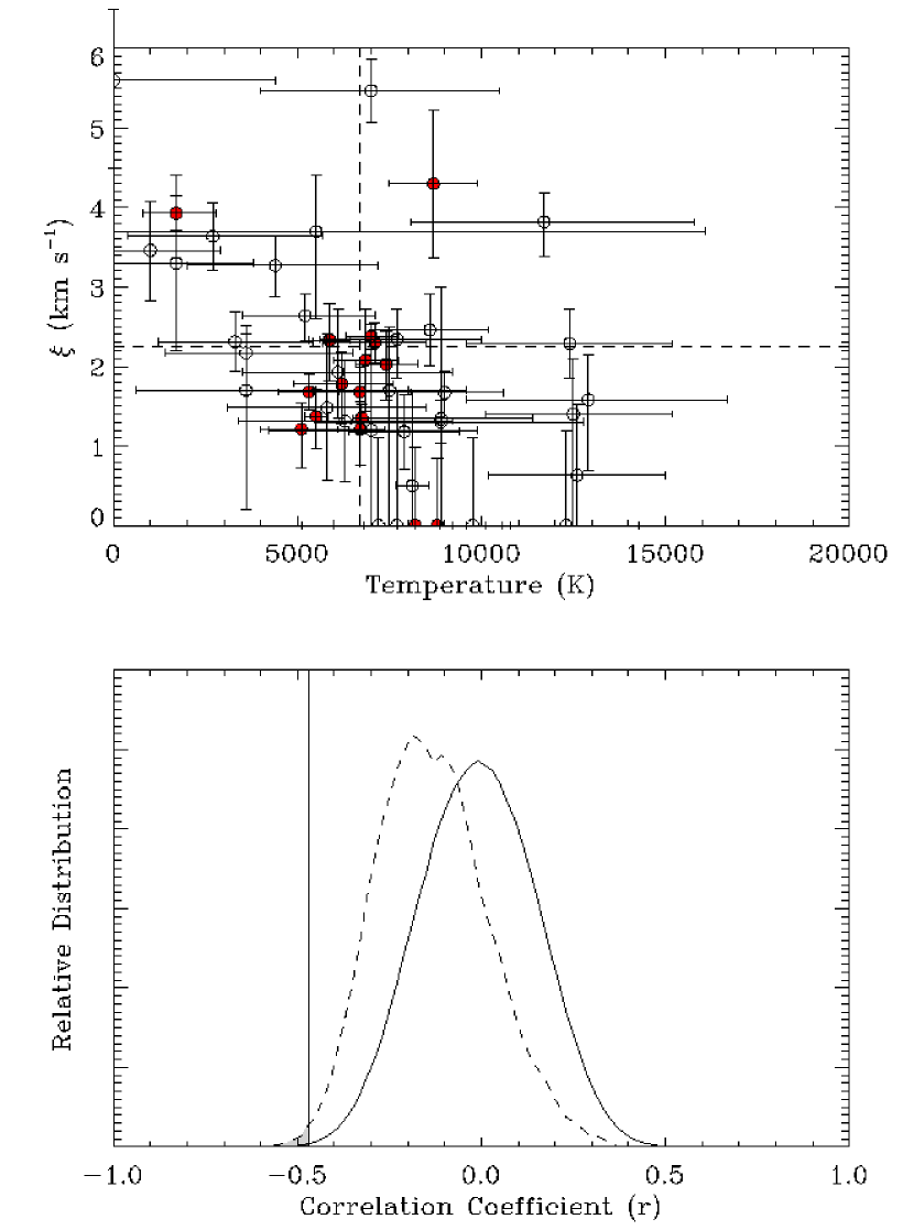
Figure 3: The top plot shows the turbulent velocity as a function of temperature for our complete sample of LISM absorbers within 100 pc. The filled symbols indicate our most precise measurements, defined by their absolute error being less than the standard deviation of the complete sample (see Figure 2). The dashed lines indicate the weighted mean values of the temperature and turbulent velocity. The bottom plot shows the distribution of correlation coefficients in $\sim\,10^{5}$ realizations of two different scenarios. The solid curve shows the distribution of a hypothetical dataset that shows no correlation, varied over the true errors, but assuming the errors in temperature and turbulence are independent and uncorrelated. The dashed curve indicates the same hypothetical sample varied according to the true error bars, but now taking into account the actual alignment of the error contours, which indicate a correlation in the errors of the variables (see error ellipses in Figure 1). For all realizations, the weighted means and dispersions of both variables ($T$ and $\xi$) were identical to the true sample. The vertical line indicates the measured correlation of our true sample. Although the probability that this value of correlation is a result of an uncorrelated parent population increases when we take into account the correlated errors (see shaded regions), the overall probability is still very low ($<\,1$ %). Therefore, the covariance between the errors of temperature and turbulence do not appear to dominate the distribution of the sample, and the moderately negative correlation between temperature and turbulence seems to be significant.

In Figure 3 the temperature and turbulence measurements are compared in aggregate for all 50 absorbers. The subsample of filled symbols indicates a selection of the most precise measurements. The $\pm\,1\sigma$ error bars of some of our measurements can span almost the entire parameter space, and therefore do not provide much insight into the physical structure of the LISM along that particular line of sight. We have therefore selected a subsample of the most precise measurements, where the absolute error is less than the standard deviation of the entire sample, given above. This subsample includes more than a third of the entire sample. There appears to be a moderate negative correlation between the temperature and turbulent velocity. The correlation coefficient ($r$) is –0.47 for the entire sample and –0.35 for the precise subsample, with the probability that the distribution could be drawn from an uncorrelated parent population ($P_{c}$) is 0.010% and 3.5%, respectively (assuming no correlation of the errors). The probability, $P_{c}$, increases when either $|r|$ or the sample size decreases.

As is evident from the alignment of the error contours in Figure 1, the majority of temperature and turbulent velocity determinations show a correlation in their measurement errors. This covariance has approximately the same alignment as the negative correlation. In other words, irrespective of the presence or absence of a negative correlation, the covariance between the errors in $T$ and $\xi$ will tend to smear out the measurements along a negatively sloped axis. To determine the significance of this effect on our sample, we calculate a large number of realizations ($\sim\,10^{5}$) for two different scenarios that have the same weighted mean and dispersion in temperature and turbulent velocity as our true dataset. A hypothetical dataset is used, which has the same number of elements as our true sample, but displays no correlation ($r\,=\,0$). Each realization is a modification of the hypothetical dataset consistent with the errors of our true sample. The two scenarios correspond to assumption that the errors are: (1) uncorrelated, where the axes of the error ellipses would be parallel to the $T$ and $\xi$ axes, and (2) correlated, as is the case for our true sample, where the error ellipses are not aligned with the principal axes. The resulting distributions are shown in the bottom of Figure 3. The first scenario (solid curve) is a distribution of samples drawn from uncorrelated errors, which as expected, peaks at $r\,\sim\,0.0$, and falls off dramatically at levels of moderate correlation ($|r|\,\sim\,0.3$). The second scenario (dashed curve) also draws from our uncorrelated hypothetical sample but is varied according to the errors, where the errors are drawn from the true covariance matrix, taking into account the correlation of measurement errors. As expected, the distribution is slightly skewed to more negative correlations, peaking at $r\,\sim\,-0.19$, due to the smearing of the sample along a negatively sloped axis. The negatively sloping error ellipses in our sample lead to a shift of any distribution of correlations to slightly more negative values, thereby increasing the probability that the observed sample could be drawn from an uncorrelated parent population. In this case, the probability increases by about a factor of 10 for the second scenario compared to the first scenario where the errors are uncorrelated (see shaded regions in Figure 3), but the overall probability still remains relatively small ($<\,1$ %). Therefore, the covariance between temperature and turbulent velocity is a minor influence on the distribution of the sample, and the negative correlation between $T$ and $\xi$ appears to be significant.

A negative correlation between our temperature and turbulent velocity measurements implies that they may not be independent variables and that either some physical phenomenon, possibly pressure equilibrium, is causing the anticorrelation, or that systematic errors in our analysis are leading to the negative correlation. Possible sources of systematic errors that are unique to each individual spectrum include the placement of the stellar continuum and the wavelength calibration. However, we expect these systematic errors to “randomize” within our sample, because they are different for each spectrum as a result of observing a variety of stars, where the location of the absorption is in a different part of the stellar continuum, and our use of different instruments with a range of spectral resolving powers. One important source of systematic error that could be ubiquitous in our sample, is the possible presence of unresolved blends. We attempt to minimize this problem by observing the narrowest LISM absorption lines at the highest available spectral resolution. However, one must consider the possible presence of several discrete absorbers with very similar projected velocities (cf. Welty, Morton, & Hobbs, 1996) and their effect on our results when we assume that there is only one absorber along the line of sight.

If unresolved blends are common in our sample, and multiple discrete absorbers are interpreted as single absorbers, then our line width measurements will be too broad. Because the unresolved blends will affect all resonance lines, independent of mass, the overestimate of the line width for each ion leads to an overestimate of the turbulent velocity. Therefore, some of the high turbulence measurements are probably due to unresolved blends rather than to intrinsically high turbulent velocities. If we neglect the turbulent velocity measurements greater than 3 km s^-1, for example, the negative correlation between temperature and turbulence is still present. The correlation coefficient is then $r\,=\,-0.35$ for the full sample and $r\,=\,-0.44$ for our best measurements subsample, and the probability ($P_{c}$) that the distribution results from an uncorrelated sample increases to 0.50% and 2.0%, respectively. The weak negative correlation may indicate a physical relationship between the temperature and turbulence in LISM clouds, perhaps involving pressure equilibrium.

3.2 Temperature, Turbulent Velocity, and Cloud Mass

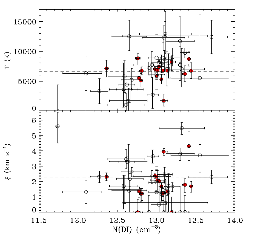
Figure 4: Cloud temperature and turbulent velocity are plotted against D I column density. The filled symbols indicate the best measurement subsample. The dashed lines indicate the weighted mean values of the temperature and turbulent velocity. The D I column density can be converted to a H I column density by applying the locally constant ratio D/H$\,=\,(1.56\,\pm\,0.04)\,\times\,10^{-5}$ (Wood et al., 2004). The hydrogen column density can be used as a proxy for the cloud mass.

The subtle connections between various cloud properties may help elucidate fundamental characteristics of interstellar gas. In Figure 4, we compare the measured temperatures and turbulent velocities with a proxy for cloud mass, the D I column density. The D I measurements are taken from Redfield & Linsky (2004). As discussed in Section 2, a line width measurement of a light ion, in particular D I, is critical for an accurate determination of cloud temperature and turbulent velocity. Therefore, a D I column density is available for all of the sightlines discussed here. The deuterium-to-hydrogen (D/H) ratio appears to be constant within the Local Bubble, D/H$\,=\,(1.56\,\pm\,0.04)\,\times\,10^{-5}$ (Wood et al., 2004). Therefore, the deuterium column density can be used to estimate the hydrogen column density, which is itself a proxy for the mass of the cloud along the line of sight, if we assume that all these clouds have comparable densities.

The plots in Figure 4 explore whether or not the temperature and turbulent velocity of the cloud vary with the cloud mass. Kinetic energy equipartition arguments suggest that, the turbulent motions of smaller clouds may be greater than those of more massive clouds. However, no correlation is discernible between column density and turbulent velocity, and equipartition does not seem to be important on the size scales of these clouds. We note that a single interstellar cloud may not have a unique turbulent velocity. Along a line of sight through an interstellar cloud, it is more likely that we are averaging over many turbulent environments within a single cloud structure, which could mask any equipartition signature. The presence of unresolved velocity structures along the line of sight could also disrupt the distribution of turbulent velocity measurements. No correlation is detected between temperature and column density either. Although the full sample seems to show a moderate positive correlation, that trend is not mirrored in the best measurement subsample, which shows no variation in $T$ or $\xi$ with column density. These comparisons seem to indicate that independent of cloud mass or size, the warm partially ionized clouds that populate the LISM share similar temperature and turbulent properties.

3.3 Cloud Structure and the Routly-Spitzer Effect

Implicit in our determination of the temperature and turbulent velocity for each component along a line of sight is the assumption that all the ions used in our analysis are members of the same collection of gas. Because all of the ions used in this paper are expected to be the dominant ionization stage, where the ionization fraction is $>50$%, for physical conditions appropriate for the LISM (Slavin & Frisch, 2002), this assumption is probably fair. Although some ions, such as, C II, Al II, Si II, and Fe II, clearly dominate the ionization distribution with $>95$% of atoms expected in their ionization stage, other ions, including, D I, N I, O I, and Mg II, have less extreme ionization fractions ranging from 55%-85%. Wood et al. (2002) used LISM column density measurements along the line of sight toward Capella to make a direct comparison between observed ionization fractions of carbon, nitrogen, and silicon, and model predictions by Slavin & Frisch (2002). If differential ionization is acting such that various ions trace distinct interstellar medium, particularly since the degree of ionization fraction dominance spans a significant range for the observed ions, the measured line widths may not fit a single temperature and turbulent velocity. We can test the assumption that the observed ions reside in the same collection of gas by looking for systematic deviations in the Doppler width of each ion compared with the trend for other ions in the same component that would arise if individual ions were sampling different environments. For example, along distant lines of sight ($\sim\,1\,$kpc), Routly & Spitzer (1952) noted that the velocity dispersion of the absorbers increased for clouds which had low Na I to Ca II ratios. This has been confirmed by more recent observations (Siluk & Silk, 1974; Vallerga et al., 1993), and is attributed to large scale structures, such as old supernova shells, that can account for both the large velocity dispersion and the change in abundance ratio. It is possible that something analogous to the Routly-Spitzer effect, whether due to varying depletion or ionization structure within an individual cloud, is acting on a much smaller scale, thereby separating the observed ions into slightly different environments within the cloud. We investigate this issue briefly here, while a detailed discussion of the ionization structure of the LISM will be provided in a subsequent paper.

In Figure 5, we test for any systematic variations by showing the weighted mean deviation for each ion from the best fit temperature and turbulent velocity solution for each cloud. The results are plotted against atomic mass as well as depletion for a typical diffuse cloud taken from the cool diffuse cloud along the $\zeta$ Oph sightline (Savage & Sembach, 1996). Although the magnitudes of the depletions of the two diffuse clouds along the line of sight toward $\zeta$ Oph are slightly offset from each other, the general trend in Figure 5 is the same regardless of which cloud is used as the depletion standard. The absorption features of both carbon and oxygen are typically saturated in our sample, which leads to their large dispersion about the weighted mean. Both deuterium and iron show very little deviation from the best fit value because they are at opposing ends of the range of atomic masses, and therefore, are the most influential in the best fit determination of the temperature and turbulent velocity. There is no indication of a systematic trend for different ions based on their depletion. In fact, the weighted mean of $\Delta$b from the best fit value is never greater than 0.1 km s^-1, which supports the assumption that these particular ions reside in the same collection of gas and provides accurate determinations of temperature and turbulent velocity.

4 Estimate of the Thermal and Turbulent Pressures in the LISM

From the distribution of the observed temperatures and turbulent velocities in the warm clouds in the LISM, we can estimate the mean thermal and turbulent pressures. The thermal pressure is defined as,

$$P_{\rm T}=nkT,$$ (4)

where $n$ is the number density of the particles in the gas, $k$ is Boltzmann’s constant, and $T$ is the gas temperature. Likewise, the turbulent pressure is defined as,

$$P_{\xi}=\frac{1}{2}\rho\xi^{2},$$ (5)

where $\rho$ is the mass density of the gas particles, and $\xi$ is the turbulent velocity of the gas. In order to calculate the gas density in the LISM, we assume cosmic abundances, or $n({\rm H})/n({\rm He})\,\sim\,10$, and that the number of electrons equals the number of protons. The electron number density is assumed to be $n_{\rm e}\,=\,0.11^{+0.12}_{-0.06}$ cm^-3, as measured for the Capella line of sight through the Local Interstellar Cloud (LIC) using the C II^∗ fine structure line (Wood & Linsky, 1997), and using a nearby white dwarf (Holberg et al., 1999). The hydrogen number density for the LISM is assumed to be $n({\rm HI})\,=\,0.1\,$cm^-3 (Redfield & Linsky, 2000). The number density ($n$) is calculated from $n\,=\,\sum\,n_{i}$, where $i$ signifies the particles included in this computation: H I ions, electrons, protons, and helium ions. Similarly, the density ($\rho$) is calculated from $\rho\,=\,\sum\,n_{i}\,m_{i}$.

Given the mean temperature of the LISM, $T\,=\,6680$ K and the measured dispersion of 1490 K, the mean thermal pressure is calculated to be $P_{\rm T}/k\,=\,2280$ K cm^-3 with a dispersion about the mean of 520 K cm^-3, which is consistent with the value $P/k=1700$ to 2300 cm^-3 K estimated by Vallerga (1996) from Extreme Ultraviolet Explorer (EUVE) spectra. The mean turbulent pressure and standard deviation, for a mean turbulent velocity of 2.24 km s^-1 and dispersion of 1.03 km s^-1, is $P_{\xi}/k\,=\,89\pm 82$ K cm^-3. The thermal pressure thus dominates the turbulent pressure, $P_{\rm T}/P_{\xi}\,\sim\,26$. Therefore, the small-scale motions in the warm clouds in the LISM, are dominated by thermal motions, as opposed to small-scale turbulence. The pressure estimates given above ignore the measurement error of $n_{\rm e}$ in order to show the magnitude of the dispersion about the weighted mean pressures. If instead, we ignore the dispersion about the mean temperature and turbulent velocity, and include the measurement error associated with $n_{\rm e}$, the measured thermal pressure is $P_{\rm T}/k\,=\,2280^{+1770}_{-880}$ K cm^-3, and the turbulent pressure is $P_{\xi}/k\,=\,89^{+36}_{-18}$ K cm^-3. Different estimates of the hydrogen number density will not change this ratio significantly because the number density essentially cancels out of the ratio.

The mean total pressure of the warm partially ionized clouds that populate the LISM is $P_{\rm tot}/k=\,P_{\rm T}/k\,+\,P_{\xi}/k\,=\,2370$ K cm^-3 with a dispersion about he mean of 530 K cm^-3. These clouds are surrounded by a larger structure, the Local Bubble, which presumably is characterized by hot ($T\,\sim\,10^{6}$ K) low density ($n_{\rm e}\,\sim\,0.005$ cm^-3) gas, which corresponds to a thermal pressure of $P_{\rm T}/k\,\sim\,11000$ K cm^-3 (Sanders et al., 1977). The pressure imbalance between the warm and hot components of the LISM has been a persistent problem for understanding the structure of our local interstellar environment (Jenkins, 2002). The present survey demonstrates that this discrepancy is common to all known local interstellar clouds within 100 parsecs, and that turbulent pressure is too small to make up the difference between the thermal pressure differences of the warm and hot LISM components. Recent results have stimulated a reexamination of the soft X-ray emission measurements of the Local Bubble, and hence the thermal pressure calculation of the hot medium. It turns out that 25-50% of the detected soft X-rays, initially wholly attributed to the hot gas in the Local Bubble, are the result of charge exchange between solar wind ions and interplanetary neutrals (Cox, 1998; Cravens, 2000; Robertson & Cravens, 2003). Therefore, the thermal pressure of the hot component of the LISM may be significantly lower than the initial estimates, and closer to agreement with the warm clouds of the LISM.

5 Turbulent Mach Number

We calculate the turbulent Mach number ($M_{\xi}$) by taking the ratio of the observed turbulent velocity to the sound speed of the gas along the line of sight,

$$M_{\xi}=\frac{\xi}{\left({\frac{nkT}{\rho}}\right)^{1/2}},$$ (6)

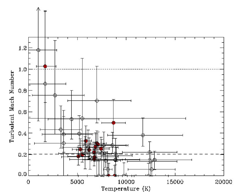
Figure 6: A plot of the turbulent Mach number as a function of cloud temperature. The gradual decrease in turbulent Mach number as a function of increasing cloud temperature is a consequence of the increase in sound speed with temperature, as well as the anticorrelation of turbulent velocity with temperature, discussed in Section 3.1. However, the vast majority of measurements, in particular the best measurement subsample, indicate a turbulent Mach number $\sim\,0.2$, shown by the dashed line. A Mach number of unity is indicated by the dotted line.

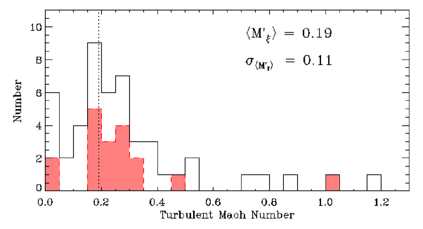
Figure 7: Distribution of the observed turbulent Mach numbers in the LISM. The weighted mean of our sample is $\langle\,M^{\prime}_{\xi}\,\rangle\,=\,$0.19, while the dispersion about the mean is 0.11. The weighted mean is indicated by a dotted line. The best measurement subsample is indicated by the shaded distribution. The high values of the turbulent Mach number may be spurious due to the possible presence of unresolved closely spaced velocity components. Turbulence in clouds within 100 pc is clearly subsonic.

where the calculation of the number density ($n$) and mass density ($\rho$) are described in Section 4. The results of this calculation are shown as a function of cloud temperature in Figure 6. The gradual decrease in turbulent Mach number as a function of increasing cloud temperature that is seen in Figure 6 is a consequence of the increase in sound speed with temperature, as well as the anticorrelation of turbulent velocity with temperature, discussed in Section 3.1. Again, the best measurement subsample is displayed as red symbols, almost all of which are clustered at a turbulent Mach number of $\sim\,0.2$. The weighted mean of the turbulent Mach number ($\langle\,M^{\prime}_{\xi}\,\rangle$) is calculated by replacing $T$ by $M_{\xi}$ in Equation 2, where $\langle\,M^{\prime}_{\xi}\,\rangle\,=\,0.19$. Similarly, the weighted dispersion about the mean value ($\sigma_{\langle\,M^{\prime}_{\xi}\,\rangle}$) is derived from Equation 3, where $\sigma_{\langle\,M^{\prime}_{\xi}\,\rangle}\,=\,0.11$. The same data are also displayed in histogram form in Figure 7. Clearly, the macroscopic nonthermal motions of warm clouds in the LISM are significantly subsonic, in contrast to the highly supersonic turbulent motions in cold neutral clouds (Heiles & Troland, 2003), and in agreement with optical observations of cool clouds (Welty, Morton, & Hobbs, 1996; Dunkin & Crawford, 1999).

6 Spatial Distribution of Temperature and Turbulent Velocity

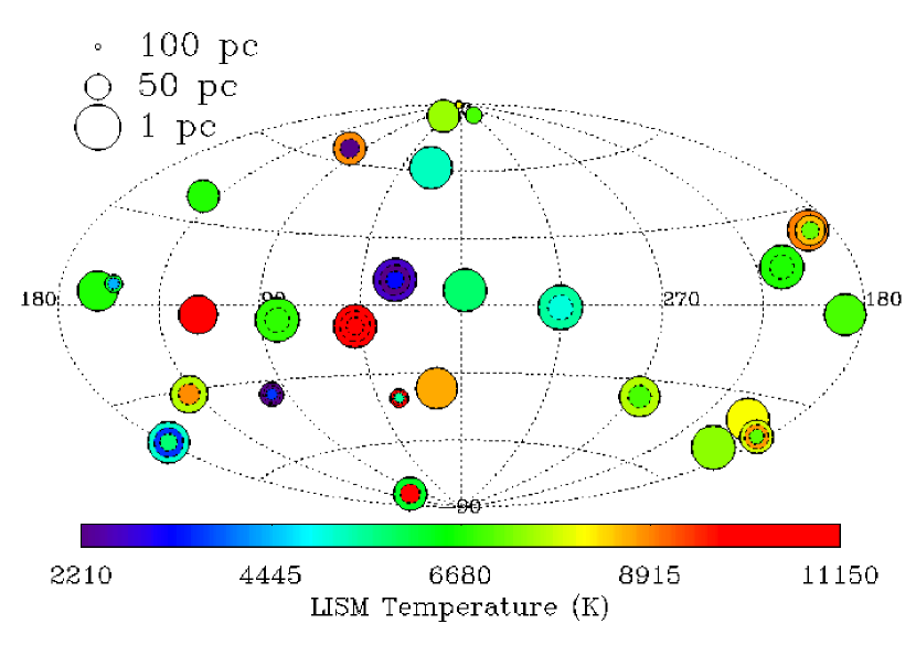
Figure 8: The spatial distribution of LISM cloud temperatures is shown in Galactic coordinates. The size of each symbol is inversely proportional to the distance, and the color of the symbol indicates the temperature of a cloud along the line of sight, as given by the scale at the bottom of the plot. If more than one absorbing cloud lies along the line of sight, additional cloud temperatures are indicated by nested circles separated by a dotted line. This technique is also used for measurements of different members of a single multiple star system, such $\alpha$ Cen. The temperatures for the two velocity components along the lines of sight to Procyon and 61 Cyg A are identical because the line widths of the closely spaced velocity components were assumed to be the same.

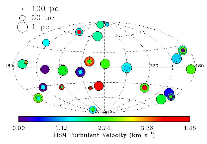
Figure 9: Similar to Figure 8, but displaying the turbulent velocity of LISM material within 100 pc.

In Figures 8 and 9, the observed temperature and turbulent velocity, respectively, for each line of sight are shown in Galactic coordinates. The size of a symbol is inversely proportional to the target’s distance, and the color of a symbol indicates the observed quantity, as shown by the scale at the bottom of each plot. Sightlines that contain more than one absorber, or sightlines to multiple targets, such as binary systems, include measurements of all clouds by separating the shadings with a dotted line. In this way, each sightline will have between one and three different shadings to signify up to three absorbers along the line of sight.

In a number of cases, both the temperature and turbulent velocity seem to be spatially correlated. For example, the closest pair of sightlines, $\alpha$ Cen A and $\alpha$ Cen B, have almost identical temperature and turbulent velocity measurements. The same is true for another close pair, Capella and the more distant white dwarf G191-B2B, which are only separated by 7^∘. The $+20$ km s^-1 component is common in the spectra of both stars, and the individual temperature and turbulent velocity measurements are practically identical. On the other hand, a closely grouped trio of stars in the direction of the North Galactic Pole, share only moderately similar cloud characteristics. With angular separations of 5^∘-8^∘, the observed spectra of 31 Com, HZ 43, and GD 153, each show one absorption component with roughly the same velocity. The derived temperature measurements are similar, ranging from 7000-8200 K, but the turbulent velocity measurements, while all less than the LISM mean, range from no detected turbulent velocity to 1.7 km s^-1 but all are formally consistent with $\xi=0.0$ km s^-1. The temperatures and turbulent velocities for the two closely spaced velocity components in the lines of sight to Procyon and 61 Cyg A are identical because the line widths were assumed to be the same due to the blending of the absorption components.

In order to quantify the magnitude of the spatial correlations in our measurements, we have compared the absolute values of the temperature and turbulent velocity differences for all unique pairings of the stars listed in Table 1. The results are plotted in Figure 10 as a function of the angular separation of the pair of sightlines, in 10^∘ bins. We also applied this procedure to the absolute values of the observed projected velocity difference ($\Delta v$) of the absorbing cloud and the total pressure, which is a function of both temperature and turbulent velocity.

It has been known for some time that the projected velocity of absorbing material in the LISM shows a strong spatial correlation (Crutcher, 1982). In fact, single three dimensional velocity vectors have been used to describe the bulk flow of the closest interstellar clouds, and is one of the predominant reasons that LISM absorbers are thought of as roughly homogeneous cloud-like entities, rather than chaotic and filamentary objects (Lallement & Bertin, 1992; Lallement et al., 1995). The spatial correlation in velocity is clearly seen in the top panel of Figure 10, where both the absolute velocity difference, and the dispersion about the weighted mean, are significantly less for sightlines with angular separations $<$ 20^∘. The dotted lines indicate the weighted mean of measurements from 0^∘-20^∘, and then from 20^∘-60^∘. The absolute value of the weighted mean velocity separation for close pairs is 21% that of more distant pairs. The same trend seems to be true for temperature, where the absolute value of the weighted mean temperature difference of pairs with separations $<$ 20^∘ is 57% of the weighted mean of more distant pairs. For turbulent velocity measurements the difference between the closest and furthest pairings is only marginal, just 81%. The total pressure of the cloud shows a significant spatial correlation, where the weighted mean of pairings $<$ 20^∘ apart is 50% of the weighted mean of pairings with greater angular separations. The spatial correlation of total pressure may be related to the negative correlation between temperature and turbulent velocity discussed in Section 3.1. Although temperature and turbulent velocity may each vary over short angular distances, pressure equilibrium may be acting to minimize the total pressure variation over small angular distances.

Temperature should be useful as a unique cloud characteristic, because like velocity the total measurement range is large but over small angular separations the mean temperature range is relatively small. However, the correlation of temperature with small angular separations is not as tight as for velocity. The turbulent velocity measurement may have less to do with the gross characteristics of a specific interstellar cloud, but could vary greatly inside a cloud from stratification of the particular physical structure of the gas due to external forces such as cloud-cloud interactions.

7 Conclusions

We present here the first systematic survey of temperature and turbulent velocity in the warm partially ionized clouds of the LISM. The collections of observations presented by Redfield & Linsky (2002, 2004), and researchers referenced therein, provide an opportunity to make fundamental physical measurements of the LISM, including 50 independent temperature and turbulent velocity measurements of the gas along 29 lines of sight in the LISM within 100 pc. The results of this work can be summarized as follows:

1. We find that in order to make an accurate and precise measurement of the gas temperature and turbulent velocity, the line widths of deuterium, and an ion at least as heavy as magnesium are required. Without deuterium there is no serious constraint on the temperature, and without a relatively heavy ion, there is no serious constraint on the turbulent velocity. High resolution observations are absolutely essential, because except for deuterium, the absorption lines are not resolved at moderate resolution, and systematic errors can dominate the measurements, leading to erroneous results.

2. The distributions of temperature and turbulent velocity of LISM gas located are both significantly peaked. The weighted mean and standard deviation for the temperature is $6680\,\pm\,1490$ K. The weighted mean and standard deviation for the turbulent velocity distribution is 2.24$\,\pm\,1.03$ km s^-1. The high turbulent velocity measurements are most likely due to unresolved blends. The standard deviation indicates the range of variation in the LISM, rather than the measurement error of the mean value. We find a significant number (18%, or between 8% and 38% including the 1$\sigma$ errors) of sightlines with temperatures $<\,5000$ K, below the stable WNM temperature regime defined by McKee & Ostriker (1977).

3. A moderately negative correlation is detected between temperature and turbulent velocity. The correlation coefficient ($r$) is –0.47 for the entire sample and –0.35 for the precise subsample, with the probability that the distribution could be from an uncorrelated parent population ($P_{c}$) of 0.010% and 3.5%, respectively. The covariance of the errors of the temperatures and turbulent velocities do not dominate the determination of this negative correlation. Pressure equilibrium among the warm clouds may be the source of this anticorrelation.

4. The small-scale thermal motions dominate the turbulent motions. For the mean temperature and turbulent velocity, we calculate a mean thermal pressure of $P_{\rm T}/k\,=$ 2280 K cm^-3 and a dispersion of 520 K cm^-3, which is consistent with the value $P/k=1700$ to 2300 cm^-3 K estimated by Vallerga (1996) from EUVE spectra. The mean thermal pressure dominates the mean turbulent pressure, $P_{\xi}/k\,=\,89$ K cm^-3 with a dispersion about the mean of 82 K cm^-3, by more than an order of magnitude, $P_{\rm T}/P_{\xi}\,\sim\,26$. Turbulent pressure in LISM clouds cannot make up the difference in the apparent pressure imbalance between warm LISM clouds and the surrounding hot gas of the Local Bubble.

5. We find that the turbulent motions of the warm partially ionized clouds in the LISM are significantly subsonic. The weighted mean and standard deviation of the turbulent Mach number for the entire sample is 0.19 $\pm$ 0.11. Although some turbulent Mach numbers approach the sound speed, due to relatively low temperatures of the clouds, these temperatures are not accurately known. The best measurement subsample clusters almost exclusively around turbulent Mach numbers of $\sim\,0.2$.

6. We have calculated the spatial distribution of the temperature and turbulent velocity for the 50 velocity components in the LISM. These individual measurements can now be combined with additional physical properties of LISM clouds, such as projected velocity and depletions, to determine the three-dimensional morphological structure of gas within 100 pc. This work will be presented in subsequent papers.

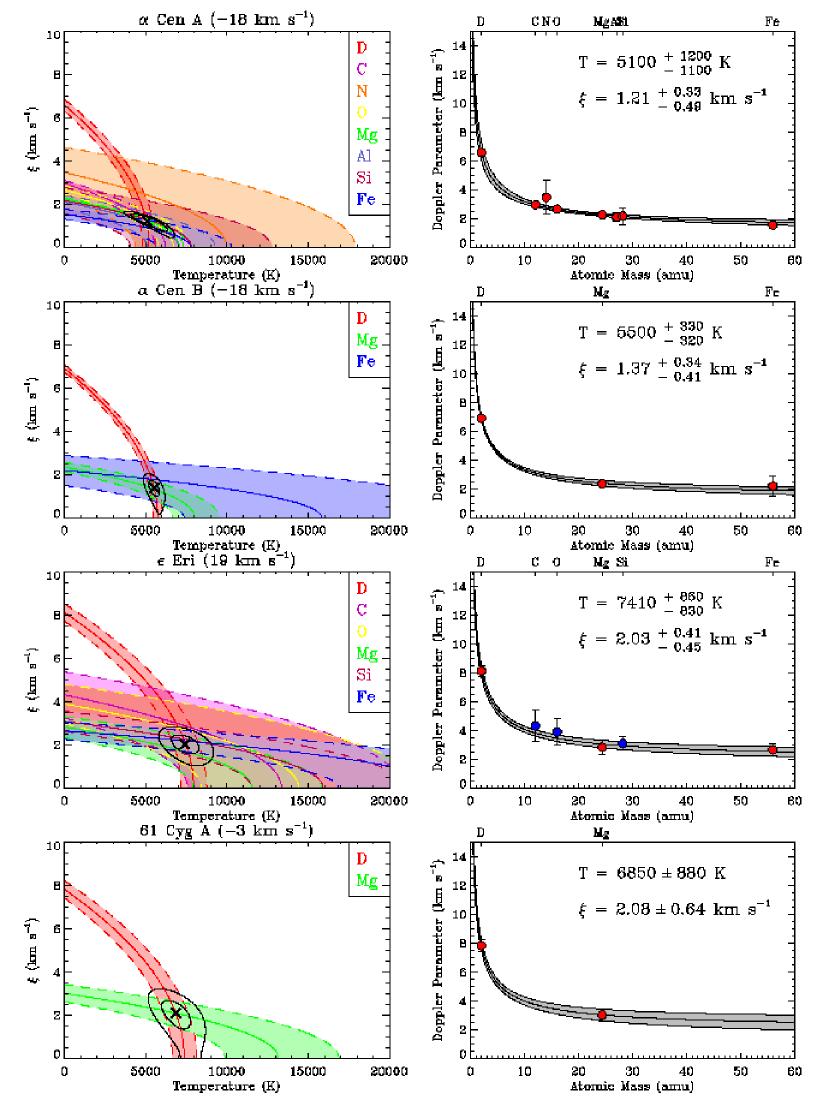
Figure 1a: Determination of the temperature ($T$) and turbulent velocity ($\xi$) for each LISM absorption component observed within 100 pc. These measurements require an observation of a light ion such as D I, and at least one other ion at least as heavy as Mg II. Each LISM component is labeled in the plot on the left with the sightline designated by the background star, and the velocity of the LISM absorption. The plot on the left shows the best fit Doppler parameter (solid lines) and $\pm\,1\sigma$ error bars (dashed lines) for each ion observed, colored coded and labeled toward the right side of the plot. Each curve is determined by the measured Doppler parameter and mass of the observed ion, as described in Equation 1. The “$\times$” symbol indicates the best fit temperature and turbulent velocity given the widths of all observed ions, while the surrounding black contours indicate the $\pm\,1\sigma$ and $\pm\,2\sigma$ error bars. The plot on the right shows the measured Doppler parameters as a function of the atomic mass of the observed ion, which are specifically indicated in the top axis. Red symbols indicate that the LISM absorption line was measured from a high resolution observation and used to make the fit, and blue symbols indicate that the measurements were from moderate resolution observations and are used as a consistency check. The best fit temperature and turbulent velocity is given in the right plot, and the best fit curve is displayed by the solid line, and the shading includes the $\pm\,1\sigma$ range of possible outcomes given the derived $T$ and $\xi$ parameters and their respective errors.

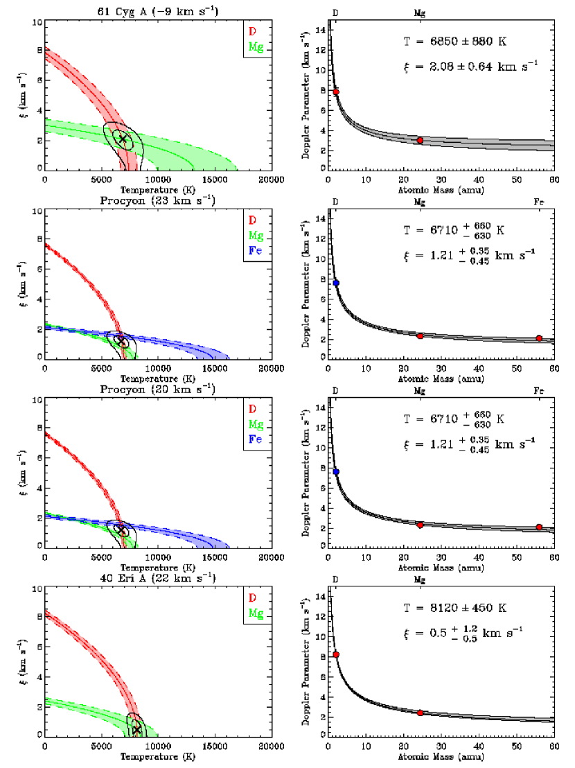
Figure 1b: Continuation of Figure 1a.

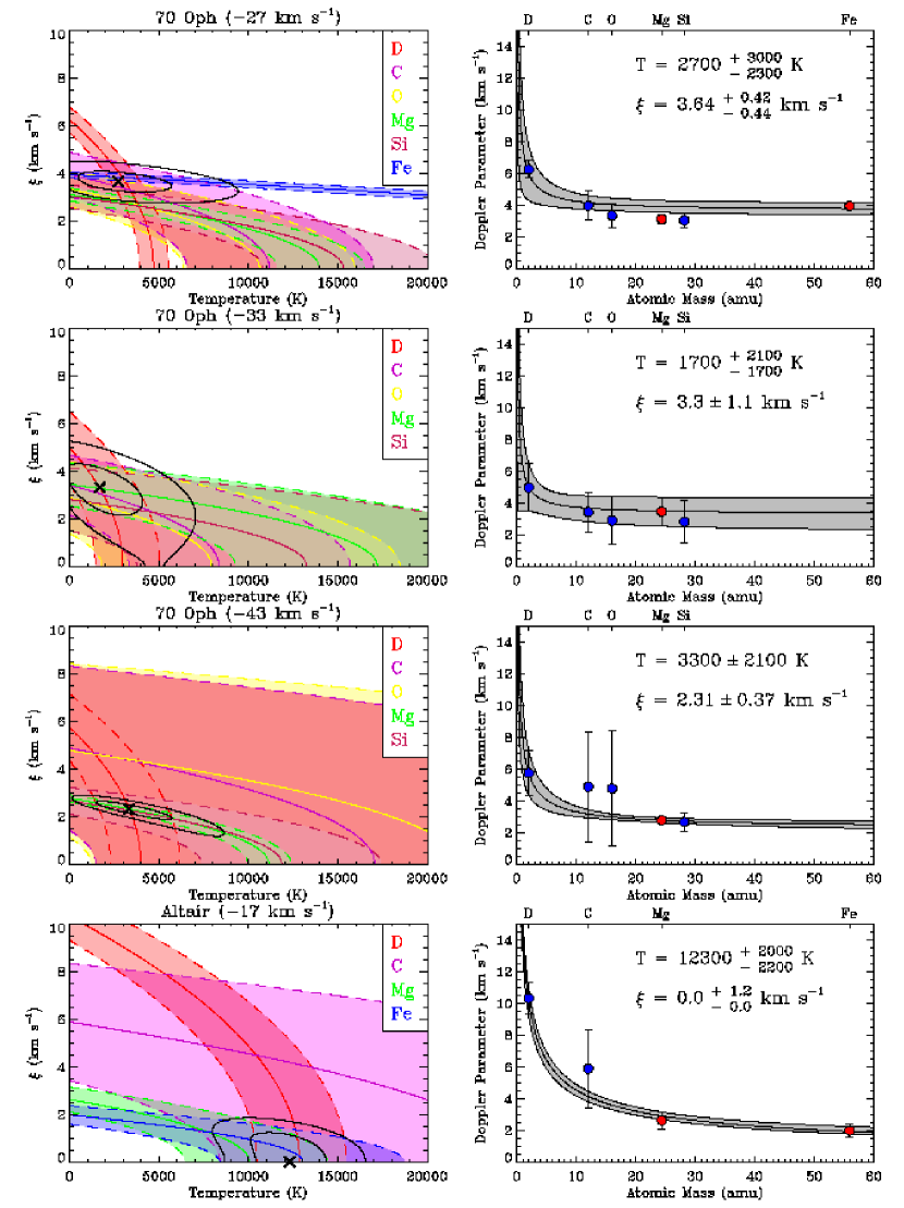
Figure 1c: Continuation of Figure 1a.

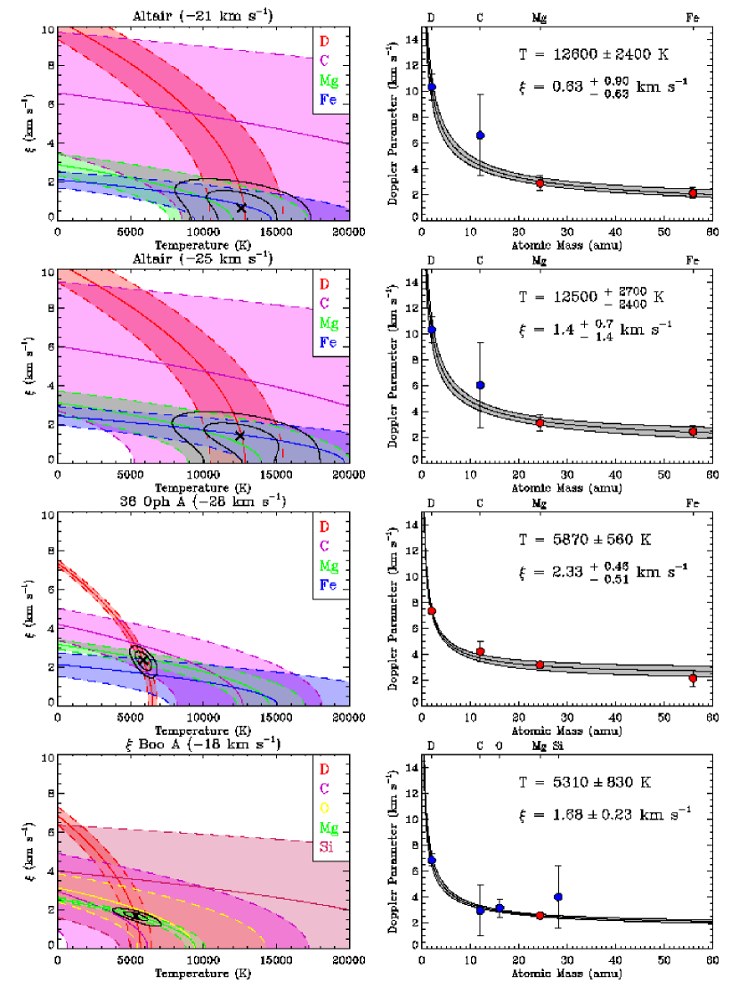
Figure 1d: Continuation of Figure 1a.

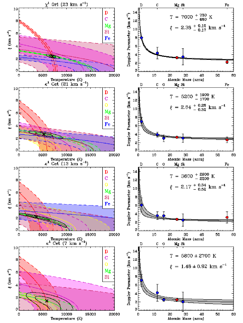
Figure 1e: Continuation of Figure 1a.

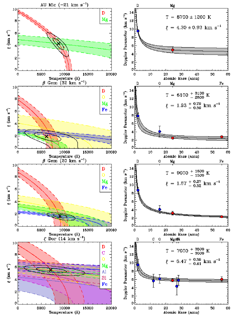
Figure 1f: Continuation of Figure 1a.

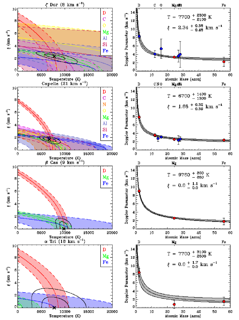
Figure 1g: Continuation of Figure 1a.

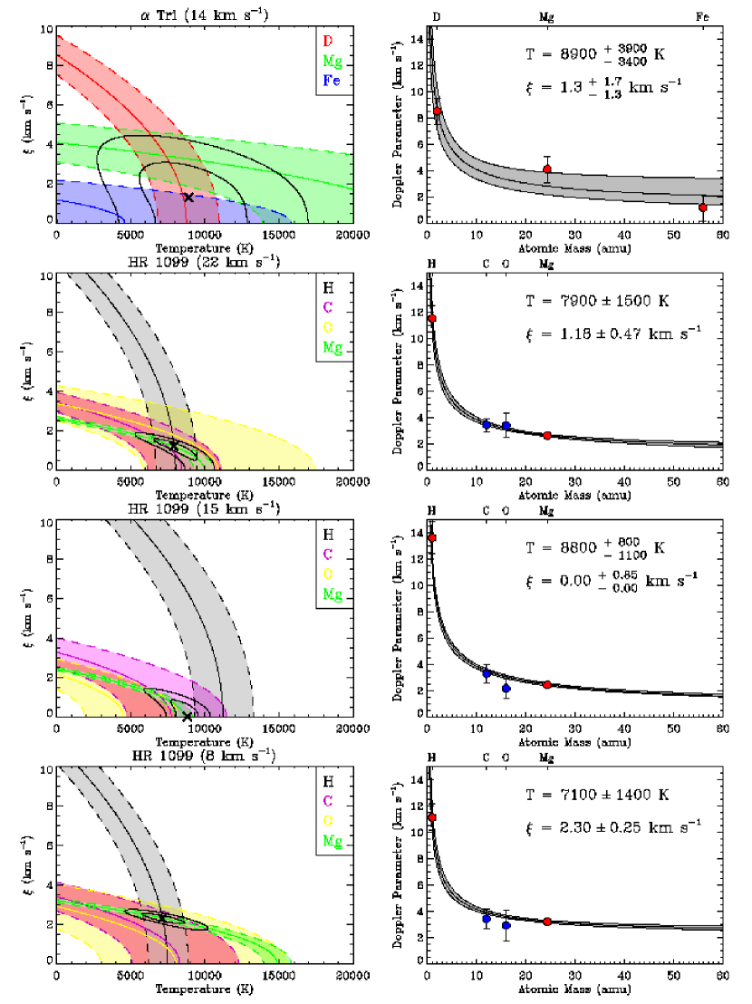
Figure 1h: Continuation of Figure 1a.

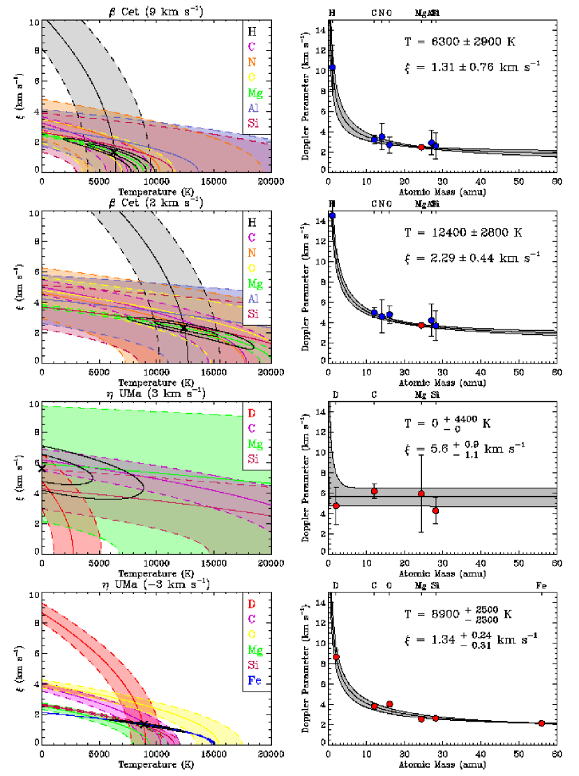
Figure 1i: Continuation of Figure 1a.

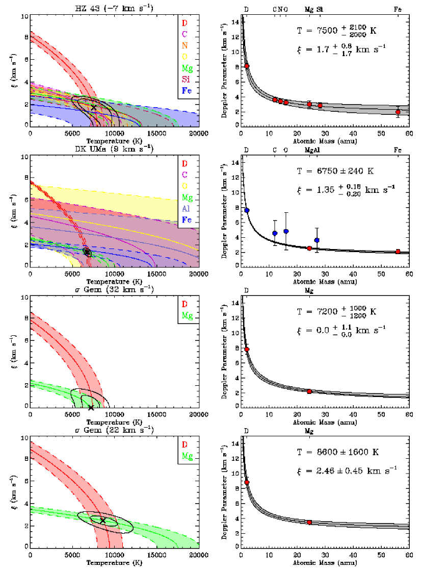
Figure 1j: Continuation of Figure 1a.

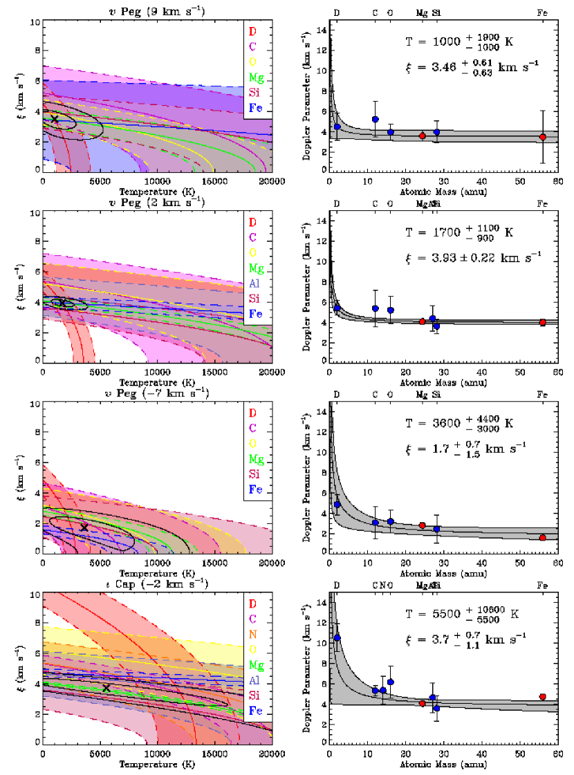
Figure 1k: Continuation of Figure 1a.

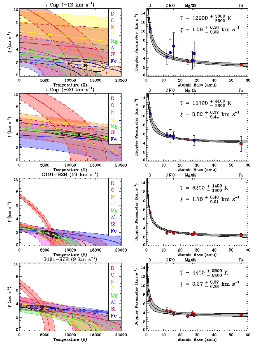
Figure 1l: Continuation of Figure 1a.

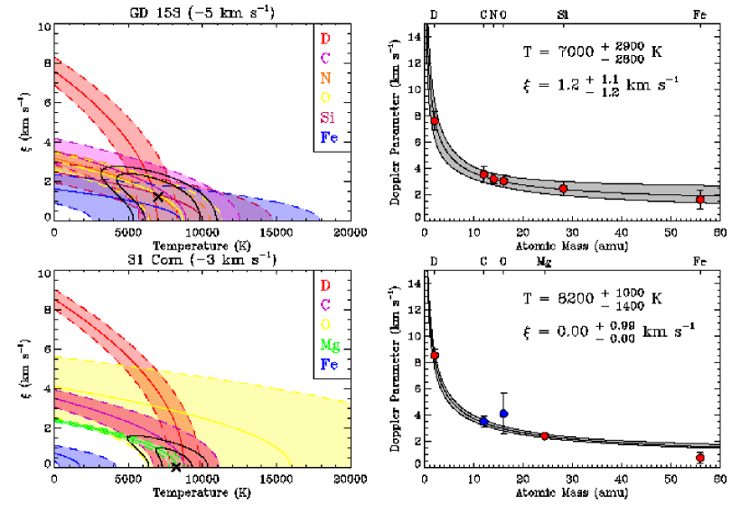
Figure 1m: Continuation of Figure 1a.

Figure 5: Departures of the weighted mean values of the Doppler parameters are compared with the best fit values for each individual ion. The top plot shows the weighted mean deviation against atomic mass, and the bottom plot shows the same against a typical depletion for each ion in the diffuse interstellar medium, taken from the cool diffuse cloud along the $\zeta$ Oph sightline (Savage & Sembach, 1996). Although the magnitudes of the depletions of the two diffuse clouds along the line of sight toward $\zeta$ Oph are slightly offset from each other, the general trend displayed here is the same regardless of which cloud is used as the depletion standard.. Carbon and oxygen have large deviations and uncertainties about the weighted mean because their absorption features are typically saturated, which inhibits a precise measurement of the Doppler parameter ($b$). No systematic trends are evident for this class of ions, supporting the assumption that they are all tracing the same collection of gas in each velocity component.

Figure 10: Differences between the measured physical parameters, velocity, temperature, turbulent velocity, and total pressure, as a function of angular separation. The bin size is 10^∘, and the weighted mean for each bin is depicted by the circle symbol, while the dispersion about the weighted mean is indicated by the error bars. On average, 20 pairings are used in each bin, while the minimum, in the 10^∘-20^∘ bin, is 6 pairings. A spatial correlation is obvious for the velocity measurements, where the absolute velocity differences, and the magnitude of the dispersion about the mean are much smaller for pairs of sightlines that are separated by 20^∘ or less. The weighted mean for separations from 0^∘-20^∘ and 20^∘-60^∘ are indicated in each plot by the dotted line. A similar spatial correlation seems to be evident in the total pressure plot, and to a lesser degree in the individual temperature and turbulent velocity plots.

Table 1: Individual Temperature and Turbulent Velocity Measurements

HD	Other	$l$	$b$	distance	$\langle v\rangle$	$T$	$\xi$	Ions used
#	Name	(∘)	(∘)	(pc)	(km s-1)	(K)	(km s-1)
128620	$\alpha$ Cen A	315.7	–0.7	1.3	–18.45 $\pm$ 0.32	5100  ${}^{+\,1200}_{-\,1100}$	1.21  ${}^{+\,0.33}_{-\,0.49}$	DI, CII, NI, OI, MgII, AlII, SiII, FeII
128621	$\alpha$ Cen B	315.7	–0.7	1.3	–18.14 $\pm$ 0.08	5500  ${}^{+\,330}_{-\,320}$	1.37  ${}^{+\,0.34}_{-\,0.41}$	DI, MgII, FeII
22049	$\epsilon$ Eri	195.8	–48.1	3.2	–18.73 $\pm$ 0.65	7410  ${}^{+\,860}_{-\,830}$	2.03  ${}^{+\,0.41}_{-\,0.45}$	DI, CII, OI, MgII, SiII, FeII
201091	61 Cyg A	82.3	–5.8	3.5	0–3.0 $\pm$ 1.4	6850 $\pm$ 880	2.08 $\pm$ 0.64	DI, MgII
					0–9.0 $\pm$ 0.7	6850 $\pm$ 880	2.08 $\pm$ 0.64	DI, MgII
61421	Procyon	213.7	13.0	3.5	023.0 $\pm$ 1.0	6710  ${}^{+\,660}_{-\,630}$	1.21  ${}^{+\,0.35}_{-\,0.45}$	DI, MgII, FeII
					019.76 $\pm$ 0.75	6710  ${}^{+\,660}_{-\,630}$	1.21  ${}^{+\,0.35}_{-\,0.45}$	DI, MgII, FeII
26965	40 Eri A	200.8	–38.1	5.0	021.73 $\pm$ 0.22	8120 $\pm$ 450	0.50  ${}^{+\,1.2}_{-\,0.5}$	DI, MgII
165341	70 Oph	29.9	11.4	5.1	–26.50 $\pm$ 0.06	2700  ${}^{+\,3000}_{-\,2300}$	3.64  ${}^{+\,0.42}_{-\,0.44}$	DI, CII, OI, MgII, SiII, FeII
					–32.53 $\pm$ 0.32	1700  ${}^{+\,2100}_{-\,1700}$	3.3 $\pm$ 1.1	DI, CII, OI, MgII, SiII
					–43.34 $\pm$ 0.14	3300 $\pm$ 2100	2.31 $\pm$ 0.37	DI, CII, OI, MgII, SiII
187642	Altair	47.7	–8.9	5.1	–17.1 $\pm$ 1.2	12300  ${}^{+\,2000}_{-\,2200}$	0.00  ${}^{+\,1.2}_{-\,0.0}$	DI, CII, MgII, FeII
					–20.9 $\pm$ 1.2	12600 $\pm$ 2400	0.630  ${}^{+\,0.90}_{-\,0.63}$	DI, CII, MgII, FeII
					–25.02 $\pm$ 0.84	12500  ${}^{+\,2700}_{-\,2400}$	1.40  ${}^{+\,0.7}_{-\,1.4}$	DI, CII, MgII, FeII
155886	36 Oph A	358.3	6.9	5.5	–28.40 $\pm$ 0.58	5870 $\pm$ 560	2.33  ${}^{+\,0.46}_{-\,0.51}$	DI, MgII, FeII
131156A	$\xi$ Boo A	23.1	61.4	6.7	–17.69 $\pm$ 0.60	5310 $\pm$ 830	1.68 $\pm$ 0.23	DI, CII, OI, MgII, SiII
39587	$\chi^{1}$ Ori	188.5	–2.7	8.7	023.08 $\pm$ 0.66	7000  ${}^{+\,730}_{-\,680}$	2.38  ${}^{+\,0.15}_{-\,0.17}$	DI, CII, MgII, SiII, FeII
20630	$\kappa^{1}$ Cet	178.2	–43.1	9.2	020.84 $\pm$ 0.20	5200  ${}^{+\,1900}_{-\,1700}$	2.64  ${}^{+\,0.28}_{-\,0.32}$	DI, CII, OI, MgII, SiII, FeII
					013.35 $\pm$ 0.15	3600  ${}^{+\,2900}_{-\,2200}$	2.17  ${}^{+\,0.34}_{-\,0.52}$	DI, CII, OI, MgII, SiII, FeII
					007.36 $\pm$ 0.46	5800 $\pm$ 2700	1.48 $\pm$ 0.92	DI, CII, OI, MgII, SiII
197481	AU Mic	12.7	–36.8	9.9	–21.45 $\pm$ 0.34	8700 $\pm$ 1200	4.30 $\pm$ 0.93	DI, MgII
62509	$\beta$ Gem	192.2	23.4	10.3	031.84 $\pm$ 0.60	6100  ${}^{+\,3100}_{-\,2600}$	1.93  ${}^{+\,0.79}_{-\,0.59}$	DI, OI, MgII, FeII
					019.65 $\pm$ 0.76	9000  ${}^{+\,1600}_{-\,1500}$	1.67  ${}^{+\,0.27}_{-\,0.32}$	DI, OI, MgII, FeII
33262	$\zeta$ Dor	266.0	–36.7	11.7	013.9 $\pm$ 1.3	7000  ${}^{+\,3500}_{-\,3000}$	5.47  ${}^{+\,0.39}_{-\,0.41}$	DI, CII, OI, MgII, AlII, SiII, FeII
					008.41 $\pm$ 0.82	7700  ${}^{+\,2300}_{-\,2100}$	2.34  ${}^{+\,0.38}_{-\,0.48}$	DI, CII, OI, MgII, AlII, SiII, FeII
34029	Capella	162.6	4.6	12.9	021.48 $\pm$ 0.51	6700  ${}^{+\,1400}_{-\,1300}$	1.68  ${}^{+\,0.32}_{-\,0.39}$	DI, CII, NI, OI, MgII, AlII, SiII, FeII
432	$\beta$ Cas	117.5	–3.3	16.7	009.15 $\pm$ 0.68	9760  ${}^{+\,800}_{-\,880}$	0.00  ${}^{+\,1.1}_{-\,0.0}$	DI, MgII, FeII
11443	$\alpha$ Tri	138.6	–31.4	19.7	017.89 $\pm$ 0.57	7700  ${}^{+\,3100}_{-\,2600}$	0.00  ${}^{+\,1.7}_{-\,0.0}$	DI, MgII, FeII
					013.65 $\pm$ 0.75	8900  ${}^{+\,3900}_{-\,3400}$	1.30  ${}^{+\,1.7}_{-\,1.3}$	DI, MgII, FeII
22468	HR 1099	184.9	–41.6	29.0	021.90 $\pm$ 0.04	7900 $\pm$ 1500	1.18 $\pm$ 0.47	HI, CII, OI, MgII
					014.80 $\pm$ 0.02	8800  ${}^{+\,800}_{-\,1100}$	0.00  ${}^{+\,0.85}_{-\,0.00}$	HI, CII, OI, MgII
					008.20 $\pm$ 0.02	7100 $\pm$ 1400	2.30 $\pm$ 0.25	HI, CII, OI, MgII
4128	$\beta$ Cet	111.3	–80.7	29.4	009.14 $\pm$ 0.21	6300 $\pm$ 2900	1.31 $\pm$ 0.76	HI, CII, NI, OI, MgII, AlII, SiII
					001.63 $\pm$ 0.22	12400 $\pm$ 2800	2.29 $\pm$ 0.44	HI, CII, NI, OI, MgII, AlII, SiII
120315	Alcaid	100.7	65.3	30.9	002.6 $\pm$ 3.4	00000  ${}^{+\,4400}_{-\,0}$	5.6  ${}^{+\,0.9}_{-\,1.1}$	DI, CII, MgII, SiII
					0–3.02 $\pm$ 0.51	8900  ${}^{+\,2500}_{-\,2300}$	1.34  ${}^{+\,0.24}_{-\,0.31}$	DI, CII, OI, MgII, SiII, FeII
	HZ 43	54.1	84.2	32.0	0–6.52 $\pm$ 0.39	7500  ${}^{+\,2100}_{-\,2000}$	1.70  ${}^{+\,0.8}_{-\,1.7}$	DI, CII, NI, OI, MgII, SiII, FeII
82210	DK UMa	142.6	38.9	32.4	009.41 $\pm$ 0.61	6750 $\pm$ 240	1.35  ${}^{+\,0.18}_{-\,0.20}$	DI, CII, OI, MgII, AlII, FeII
62044	$\sigma$ Gem	191.2	23.3	37.5	032.26 $\pm$ 0.15	7200  ${}^{+\,1000}_{-\,1200}$	0.00  ${}^{+\,1.1}_{-\,0.0}$	DI, MgII
					021.77 $\pm$ 0.16	8600 $\pm$ 1600	2.46 $\pm$ 0.45	DI, MgII
220657	$\upsilon$ Peg	98.6	–35.4	53.1	008.8 $\pm$ 1.2	001000  ${}^{+\,1900}_{-\,1000}$	3.46  ${}^{+\,0.61}_{-\,0.63}$	DI, CII, OI, MgII, SiII, FeII
					001.73 $\pm$ 0.39	1700  ${}^{+\,1100}_{-\,900}$	3.93 $\pm$ 0.22	DI, CII, OI, MgII, AlII, SiII, FeII
					0–7.48 $\pm$ 0.43	3600  ${}^{+\,4400}_{-\,3000}$	1.7  ${}^{+\,0.7}_{-\,1.5}$	DI, CII, OI, MgII, SiII, FeII
203387	$\iota$ Cap	33.6	–40.8	66.1	0–2.22 $\pm$ 0.19	5500  ${}^{+\,10600}_{-\,5500}$	3.7  ${}^{+\,0.7}_{-\,1.1}$	DI, CII, NI, OI, MgII, AlII, SiII, FeII
					–12.06 $\pm$ 0.49	12900  ${}^{+\,3800}_{-\,3300}$	1.580  ${}^{+\,0.56}_{-\,0.89}$	DI, CII, NI, OI, MgII, AlII, SiII, FeII
					–20.48 $\pm$ 0.45	11700  ${}^{+\,4100}_{-\,3600}$	3.82  ${}^{+\,0.37}_{-\,0.44}$	DI, CII, NI, OI, MgII, SiII, FeII
	G191-B2B	156.0	7.1	68.8	019.19 $\pm$ 0.15	6200  ${}^{+\,1400}_{-\,1300}$	1.78  ${}^{+\,0.40}_{-\,0.51}$	DI, CII, NI, OI, MgII, AlII, SiII, FeII
					008.61 $\pm$ 0.38	4400  ${}^{+\,2800}_{-\,2400}$	3.27  ${}^{+\,0.37}_{-\,0.39}$	DI, CII, NI, OI, MgII, AlII, SiII, FeII
	GD 153	317.3	84.8	70.5	0–5.04 $\pm$ 0.17	7000  ${}^{+\,2900}_{-\,2800}$	1.20  ${}^{+\,1.1}_{-\,1.2}$	DI, CII, NI, OI, SiII, FeII
111812	31 Com	115.0	89.6	94.2	0–3.37 $\pm$ 0.37	8200  ${}^{+\,1000}_{-\,1400}$	0.00  ${}^{+\,0.99}_{-\,0.00}$	DI, CII, OI, MgII, FeII

Note. — This table includes only those measurements that include independent fits to the line width of deuterium and an ion at least as heavy as magnesium.

References

- Bevington & Robinson (1992) Bevington, P.R., & Robinson, D.K. 1992, Data Reduction and Error Analysis for the Physical Sciences (New York: McGraw-Hill) 2004, in How the Galaxy Works - Galactic Tertulia: A Tribute to Don Cox and Ron Reynolds”, ed. E.J Alfaro, E. Perez, J. Franco (Dordrecht: Kluwer), in press (astro-ph/0401428)
- Cox (1995) Cox, D. 1995, Nature, 375, 185
- Cox (1998) Cox, D. 1998, in IAU Colloq. 166, The Local Bubble and Beyond, ed. D. Breitschwerdt, M.J. Freyberg, & J. Trümper (Berlin: Springer-Verlag), 121
- Cravens (2000) Cravens, T.E. 2000, ApJ, 532, L153
- Crutcher (1982) Crutcher, R.M. 1982, ApJ, 254, 82
- Dunkin & Crawford (1999) Dunkin, S.K., & Crawford, I.A. 1999, MNRAS, 302,197
- Field, Goldsmith, & Habing ( 1969) Field, G.B., Goldsmith, D.W., & Habing, H.J. 1969, ApJ, 155, L149 2002]frisch02 Frisch, P.C., Grodnicki, L., & Welty, D.E. 2002, ApJ, 574, 834
- Heiles (2001a) Heiles, C. 2001, in ASP Conf. Ser., Vol. 231, Tetons4: Galactic Structure, Stars, and the Interstellar Medium, ed. C.E. Woodward, M.D. Bicay, & J.M. Shull (San Francisco: PASP), 294
- Heiles (2001b) Heiles, C. 2001, ApJ, 551, L105
- Heiles & Troland (2003) Heiles, C., & Troland, T.H. 2003, ApJ, 586, 1067
- Holberg et al. (1999) Holberg, J.B., Bruhweiler, F.C., Barstow, M.A., & Dobbie, P.D. 1999, ApJ, 517, 841
- Hurwitz & Sholl (1999) Hurwitz, M., & Sholl, M. 1999, BAAS, 31, 1505
- Jenkins (2002) Jenkins, E.B. 2002, ApJ, 580, 938
- Jenkins & Tripp (2001) Jenkins, E.B., & Tripp, T.M. 2001, ApJS, 137, 297
- Lallement & Bertin (1992) Lallement, R., & Bertin, P. 1992, A&A, 266, 479 R., Vidal-Madjar, A., & Bertaux, J.L. 1994, A&A, 286, 898
- Lallement et al. (1995) Lallement, R., Ferlet, R., Lagrange, A.M., Lemoine, M., & Vidal-Madjar, A. 1995, A&A, 304, 461
- Lallement et al. (2003) Lallement, R., Welsh, B.Y., Vergely, J.L., Crifo, F., & Sfeir, D. 2003, A&A, 411, 447
- Linsky & Wood (1996) Linsky, J.L., & Wood, B.E. 1996, ApJ, 463, 254
- McKee & Ostriker (1977) McKee, C.F., & Ostriker, J.P. 1977, ApJ, 218, 148
- Piskunov et al. (1997) Piskunov, N., Wood, B.E., Linsky, J.L., Dempsey, R.C., & Ayres, T.R. 1997, ApJ, 474, 315
- Redfield & Linsky (2000) Redfield, S., & Linsky, J.L. 2000, ApJ, 534, 825 J.L. 2001, ApJ, 551, 413
- Redfield & Linsky (2002) Redfield, S., & Linsky, J.L. 2002, ApJS, 139, 439
- Redfield & Linsky (2004) Redfield, S., & Linsky, J.L. 2004, ApJ, 602, 776
- Robertson & Cravens (2003) Robertson, I.P., & Cravens, T.E. 2003, J. Geophys. Res., 108(A10), 8031
- Routly & Spitzer (1952) Routly, P.M., & Spitzer, L., Jr. 1952, ApJ, 115, 227
- Sanders et al. (1977) Sanders, W.T., Kraushaar, W.L., Nousek, J.A., & Fried, P.M. 1977, ApJ, 217, L87
- Savage & Sembach (1996) Savage, B.D., & Sembach, K.R. 1996, ARA&A, 34, 279
- Sfeir et al. (1999) Sfeir, D.M., Lallement, R., Crifo, F., & Welsh, B.Y. 1999, A&A, 346, 785
- Slavin & Frisch (2002) Slavin, J.D., & Frisch, P.C. 2002, ApJ, 565, 364
- Snowden et al. (1998) Snowden, S.L., Egger, R., Finkbeiner, D., Freyberg, M., & Plucinsky, P. 1998, ApJ, 493, 715
- Siluk & Silk (1974) Siluk, R.S., & Silk, J. 1974, ApJ, 192, 51
- Vallerga (1996) Vallerga, J. 1996, Space Sci. Rev., 78, 277
- Vallerga et al. (1993) Vallerga, J.V., Vedder, P.W., Craig, N., & Welsh, B.Y. 1993, ApJ, 411, 729
- Welsh et al. (1994) Welsh, B.Y., Craig, N., Vedder, P.W., & Vallerga, J.V. 1994, ApJ, 437, 638
- Welty et al. (2002) Welty, D.E., Jenkins, E.B., Raymond, J.C., Mallouris, C., & York, D.G. 2002, ApJ, 579, 304
- Welty, Morton, & Hobbs (1996) Welty, D.E., Morton, D.C., & Hobbs, L.M. 1996, ApJS, 106, 533
- Wolfire et al. (1995a) Wolfire, M.G., Hollenbach, D., McKee, C.F., Tielens, A.G.G.M., & Bakes, E.L.O. 1995a, ApJ, 443, 152
- Wolfire et al. (1995b) Wolfire, M.G., McKee, C.F., Hollenbach, D., & Tielens, A.G.G.M. 1995b, ApJ, 453, 673
- Wood & Linsky (1997) Wood, B.E., & Linsky, J.L. 1997, ApJ, 474, L39
- Wood et al. (2004) Wood, B.E., Linsky, J.L., Hébrard, G., Williger, G.M., Moos, H.W., & Blair, W.P. 2004, ApJ, in press
- Wood, Linsky, & Zank (2000) Wood, B.E., Linsky, J.L., & Zank, G.P. 2000, ApJ, 537, 304
- Wood et al. (2002) Wood, B.E., Redfield, S., Linsky, J.L., & Sahu, M.S. 2002, ApJ, 581, 1168