New spectral classification technique for X-ray sources: quantile analysis

Abstract

We present a new technique called quantile analysis to classify spectral properties of X-ray sources with limited statistics. The quantile analysis is superior to the conventional approaches such as X-ray hardness ratio or X-ray color analysis to study relatively faint sources or to investigate a certain phase or state of a source in detail, where poor statistics does not allow spectral fitting using a model. Instead of working with predetermined energy bands, we determine the energy values that divide the detected photons into predetermined fractions of the total counts such as median (50%), tercile (33% & 67%), and quartile (25% & 75%). We use these quantiles as an indicator of the X-ray hardness or color of the source. We show that the median is an improved substitute for the conventional X-ray hardness ratio. The median and other quantiles form a phase space, similar to the conventional X-ray color-color diagrams. The quantile-based phase space is more evenly sensitive over various spectral shapes than the conventional color-color diagrams, and it is naturally arranged to properly represent the statistical similarity of various spectral shapes. We demonstrate the new technique in the 0.3-8 keV energy range using Chandra ACIS-S detector response function and a typical aperture photometry involving background subtraction. The technique can be applied in any energy band, provided the energy distribution of photons can be obtained.

1 Introduction

A major obstacle for understanding the nature of the faintest X-ray sources is poor statistics, which prevents the usual practice of spectral analysis such as fitting with known models. Even for apparently bright sources, as we investigate the sources in detail, we frequently need to divide source photons in various phases or states of the sources and the success of such an analysis is often limited by statistics. The common practice to extract spectral properties of X-ray sources with poor statistics is to calculate X-ray hardness or color of the sources (e.g. Schulz et al., 1989; Kim et al., 1992; Netzer et al., 1994; Prestwich et al., 2003). In this conventional method, the full-energy range is divided into two or three sub-bands and the detected source photons are counted separately in each band. The ratio of these counts is defined as X-ray hardness or color, to serve as an indicator of the spectral properties of the source.

In principle, one can constrain a meaningful X-ray hardness or color to a source if at least one source photon is detected in each of at least two bands. However, the equivalent requirement for total counts in the full-energy band can be rather demanding and it is strongly spectral dependent. Fig. 1 shows an example of a X-ray color-color diagram (Kim et al., 2003). In the figure, we divide the full-energy range (0.3-8.0 keV) into three sub-energy bands; 0.3-0.9 (S), 0.9-2.5 (M), and 2.5-8.0 keV (H). The ratio of the net source counts in S to M band is defined as the soft X-ray color ($x$-axis in the figure), and the ratio of the net counts in M to H band as the hard X-ray color ($y$-axis). The energy range in this example is the region where the Chandra ACIS-S detectors are sensitive, but the technique described in this paper is not bounded to any particular energy range, provided the energy distribution of photons can be obtained.

The grid pattern in the figure represents the true location for the sources with the power-law spectra governed by two parameters: power-law index ($\Gamma$) and absorbing column depths ($N\mbox{$\rm{}_{H}$}$) along the line of the sight. The grid pattern is drawn for an ideal detector response, which is constant over the full-energy band. The grid pattern appears to be properly spaced to the changes of the spectral parameters and such an arrangement suggests that this color-color diagram may be an ideal way to classify sources with poor statistics.

However, the appearance can be deceiving, which is hinted by the uneven sizes of error bars in the figure. The error bar near each grid node represents the central 68% of simulation results from the spectral shape at the grid node. Each simulation has 1000 source counts in the full-energy range with no background counts, and thus the size of the symbol represents the size of typical error bars for 1000 count sources in the diagram.

In the figure, there are two kinds of error bars for some spectral shapes (e.g. $\Gamma$ = 0 and $N\mbox{$\rm{}_{H}$}$ = $10^{22}$ cm^-2); the thick error bars represent the central 68% distribution of the simulation results that have “proper” color values (defined here as at least one photon in each of all three bands), and the thin error bars show the 68% distribution of all the simulation trials (10,000) for each spectral model, i.e. a distribution of the central 6827 trials. The two error bars should be identical if all the trials produce a proper soft and hard color.

The right panel in Fig. 1 shows the minimum counts in the full-energy band to have at least one count in each of three bands. The figure indicates that the required minimum counts are dramatically different among the models in the grid. For the power-law spectra with $\Gamma$ = 0 and $N\mbox{$\rm{}_{H}$}$ $\sim 10^{22}$ cm^-2, more than 500 counts are required in order to have reasonable color values, while in the case of $\Gamma$ = 2 and $N\mbox{$\rm{}_{H}$}$ $\sim 10^{20}$ cm^-2, a few counts are sufficient. Because of statistical fluctuations, for some models, even 1000 counts in the full-energy range do not guarantee positive net counts in all three bands, which explains why some trials fail to produce proper colors.

The spectral-model dependence of error bars in this kind of color-color diagram is inevitable and the dependence is determined by the choice of the sub-energy bands for a full-energy range. In this example, the sub bands are chosen so that the diagram is mostly sensitive near $\Gamma$ = 2 and $N\mbox{$\rm{}_{H}$}$ $<10^{22}$ cm^-2. In fact, it is not possible to select sub bands to have uniform sensitivity over different spectral shapes.

Fig. 1 clearly indicates that the conventional color-color diagram (CCCD) is heavily biased, which is very unfortunate when trying to extract unknown spectral properties from the sources. The heavy requirement on the total counts for certain spectral shapes defeats the purpose of the diagram since the large total counts may allow nominal spectral analysis such as spectral fitting with known models. One might have to repeat the analysis with different choices of sub-bands to explore all the interesting possibilities of spectral shapes.

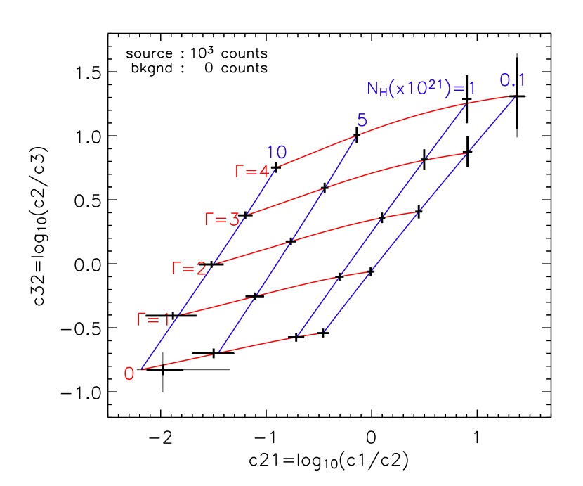
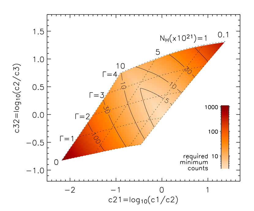
Figure 1: Conventional color-color diagram (CCCD): two colors are defined by the net counts (c1, c2, and c3) in three energy bands (0.3-0.9, 0.9-2.5, and 2.5-8.0 keV). The left panel shows simulation results of 20 spectral shapes for an ideal detector with a uniform response function. The error bar represents the central 68% of simulation results for each of 20 power-law spectra governed by two parameters – power-law index ($\Gamma$) and column depth ($N\mbox{$\rm{}_{H}$}$) along the line of the sight. The thick error bars are for the 68% of the cases with proper color values (at least one count in each of the three bands) and the thin error bars for considering 10,000 trials (see text). Each simulation run contains 1000 source counts in the full 0.3-8.0 keV energy range. In this example, the two error bars are identical except for the case of $\Gamma$ =0 & $N\mbox{$\rm{}_{H}$}$ =10²² cm^-2 and $\Gamma$ =4 & $N\mbox{$\rm{}_{H}$}$ =10²⁰ cm^-2, where many simulation runs result in null count in at least one of sub-bands. The grid pattern represents the true location of these spectra in the diagram. The right panel shows the required minimum counts in the full-energy band in order to have at least one count in each of three bands. The contour lines quantize the gray (color) scale for easier interpretation. See electronic ApJ for color version of the figure as well as other figures.

2 Quantiles

In order to overcome the selection effects originating from the predetermined sub-energy bands, we propose to use the energy value to divide photons into predetermined fractions. We choose fractions to take full advantage of the given statistics, such as 50% (median), 33% & 67% (tercile), and 25% & 75% (quartile), although any quantile may be used. We use the corresponding energy values - quantiles - as an indicator of the X-ray hardness or color of the source. In particular, we will show below that the median, $Q_{50}$, is an improved substitute for the conventional X-ray hardness.

Let $E_{x\%}$ be the energy below which the net counts is $x\%$ of the total counts and we define quantile $Q_{x}$

$$\mbox{$Q_{x}$}=\frac{\mbox{$E_{x\%}$}-E\mbox{$\rm{}_{lo}$}}{E\mbox{$\rm{}_{up}$}-E\mbox{$\rm{}_{lo}$}},$$

where $E\mbox{$\rm{}_{lo}$}$ and $E\mbox{$\rm{}_{up}$}$ is the lower and upper boundary of the full-energy band respectively (0.3 and 8.0 keV in this example). The algorithm for estimation of quantiles and their errors relevant to X-ray astronomy is given in the appendix. Unlike the conventional X-ray hardness or colors, for calculating quantiles, there is no spectral dependence of required minimum counts. The required minimum only depends on types of quantiles: two counts for median and terciles, and three for quartiles.

Fig. 2 shows an example of quantile-based color-color diagrams (QCCDs) using the median $m(\equiv\mbox{$Q_{50}$})$ for the $x$-axis and the ratio of two quartiles $Q_{25}$/$Q_{75}$ for the $y$-axis (see §5 for the motivation of the choice of the axes). The grid pattern in Fig. 2 is drawn for the same spectral parameters as in Fig. 1 with five additional cases for $N\mbox{$\rm{}_{H}$}$ = $5\times 10^{22}$ cm^-2. Note that the approximate axes of $\Gamma$ and $N\mbox{$\rm{}_{H}$}$ are rotated $\sim$ 90$\deg$ from those in Fig. 1. The error bars are drawn for the central 68% of the same 10,000 simulation results of the spectral shape at each grid node, and each simulation run contains 1000 source counts with no background counts in the full-energy band. The relatively similar size of the error bars for 1000 count sources in the figure indicates that there is no spectral dependent selection effect. Note that there is no need of distinction for thin and thick error bars in this figure because all the trials produce proper quantiles.

The grid pattern of power-law spectra in Fig. 2 appears to be less intuitively arranged than the one in Fig. 1. However, we believe that the proximity of any two spectra in the quantile-based diagram accurately exhibits the similarity of the two spectral shapes (as folded through the detector response, which is constant in this example). For example, in the case for $\Gamma$ = 0 in Fig. 2, the separation in phase space by various $N\mbox{$\rm{}_{H}$}$ values is much smaller than in the case for $\Gamma$ $\geq$ 1. Note that the column depth ($N\mbox{$\rm{}_{H}$}$) in the considered range can change mainly soft X-rays ($\lesssim$ 2 keV) and the spectrum for $\Gamma$ = 0 is less dominated by soft X-rays than that for $\Gamma$ $\geq$ 1. In other words, the overall effects of $N\mbox{$\rm{}_{H}$}$ on the spectral shape would be much smaller in the case for $\Gamma$ = 0 than in the case for $\Gamma$ $\geq$ 1. Therefore, the grid spacing in Fig. 2 indeed reveals the appropriate statistical power needed to discern these spectral shapes, despite the degeneracy arising from utilizing only three variables (quantiles) extracted from a spectrum.

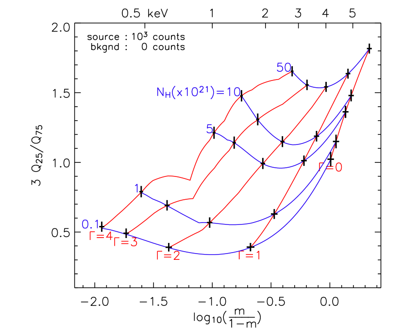
Figure 2: Same as Fig. 1 but quantile-based color-color diagram (QCCD) based on the median $Q_{50}$ and the ratio of two quartiles $Q_{25}$/$Q_{75}$. See §5 for the origin of the logarithmic form for the $x$-axis. The energy scale across the top shows the median energy values ($E_{50\%}$). The simulation results are given from the same simulation sets in Fig. 1 (1000 source counts). Note that there are five more spectral shapes with $N\mbox{$\rm{}_{H}$}$ = $5\times 10^{22}$ cm^-2 than in Fig. 1. The grid pattern represents the true location of these spectra in the diagram for an ideal detector. Note the relative uniformity of error bars, compared to Fig. 1.

3 Color-color diagram example

Now let us consider more realistic examples. We introduce the Chandra ACIS-S response function; we use the pre-flight calibration data for energy resolution and the energy dependent effective area from PIMMS version 2.3.

Fig. 3 shows the simulation results of the spectra with 100 and 50 source counts with no background counts. The error bars again indicate the interval that encloses the central 68% of the simulation results for each model. The results are shown for both the conventional and new color-color diagrams in the figure. The grid patterns in the figures are for the same power-law models and they look different from the previous examples because of the Chandra ACIS-S response function.

The analysis of faint sources is often limited by background fluctuations. In contrast to Fig. 3, we allow for large background counts in the source region (e.g. a point source in a bright diffuse emission region). The top two panels in Fig. 4 shows the simulation results of the spectra with 100 source counts and 50 background counts in the source region, and the bottom two panel shows the case of 50 source counts and 25 background counts. For background subtraction, we set the background region to be five times larger than the source region. The background region contains 250 (top panels) and 125 background (bottom panels) counts respectively. Note these are relatively high backgrounds for a typical Chandra source and thus illustrate the worst case of a point source superimposed in background diffuse emission. The background photons are sampled from a power-law spectrum with $\Gamma$ = 0 and $N\mbox{$\rm{}_{H}$}$ = 0, which is folded through the Chandra ACIS-S response function.

In the case of the CCCD in Figs. 3 and 4, one can notice that some of the error bars lie away from their true location (grid node). The severe requirement for the total counts ($>100$) for some of the spectral models results in only a lower or upper limit for the color in many simulation runs. Cases with proper colors for these models are greatly influenced by statistical fluctuations because of low source counts in one or two sub-bands, and thus the estimated colors fail to produce the true value. It is evident that this conventional diagram is more sensitive towards $\Gamma$ $\sim$ 2 and $N\mbox{$\rm{}_{H}$}$ $\lesssim 10^{22}$ cm^-2.

In the case of the new quantile-based diagram, the error bars stay at the correct location and the size of the error bars are relatively uniform across the model phase space, indicating that the phase space is properly arranged. The quantile-based diagram shows more consistent results regardless of background.

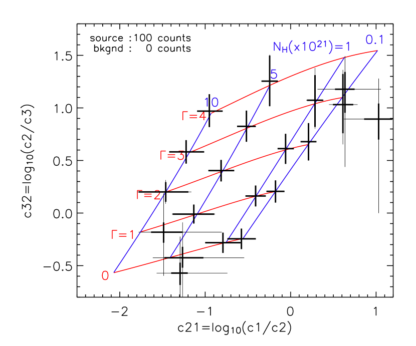
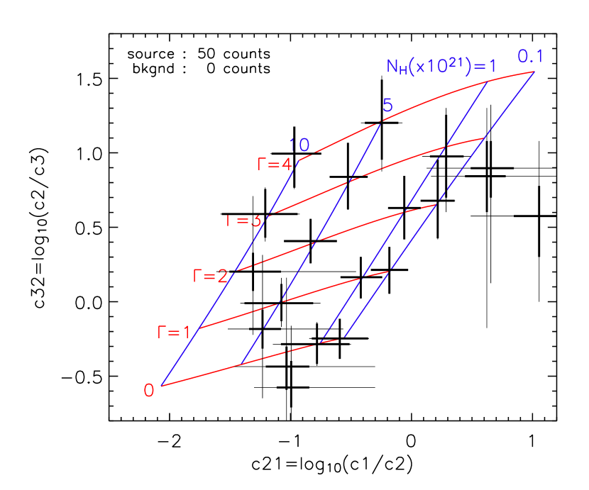
Figure 3: Realistic example of the color-color diagram with no background: 100 (top panels) and 50 (bottom panels) source counts for each spectral model folded through the Chandra ACIS-S response function. The left two panels show the CCCD and the right two panels show the QCCD. The grid pattern of both cases are different from the previous example because of the ACIS-S response function. In the case of the CCCD, the average of the simulation results are often severely different from the true value (grid node) due to the selection effect inherent to the band choice. The selection effect also causes the large difference between thick and thin error bars, which indicates that only a fraction of simulations produce proper colors. The fraction can be even smaller than 68% of the total 10,000 runs, in which case the thin error bar represents the full range of the simulation outcomes with proper colors. The quantile-based diagram provides the correct results regardless of spectral shapes.

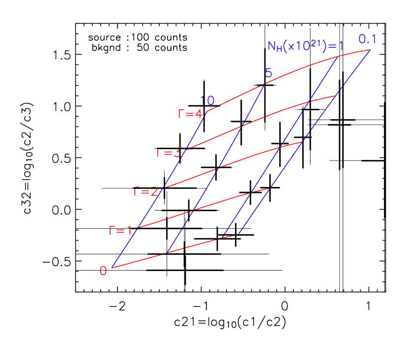
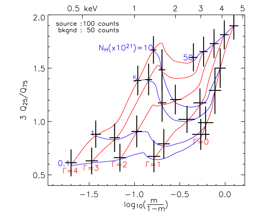
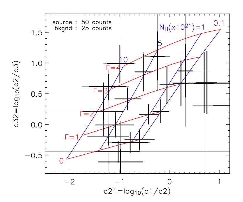
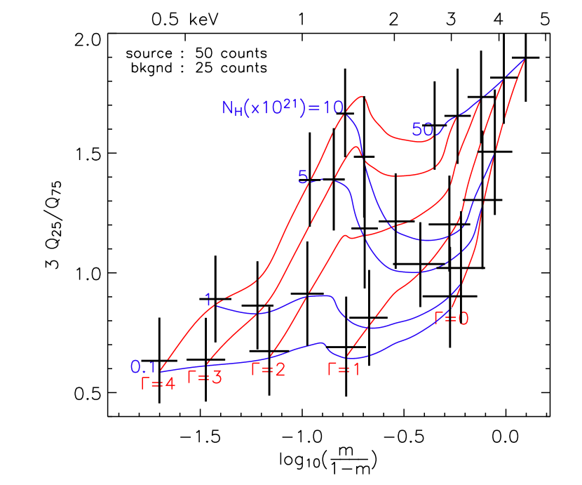
Figure 4: Realistic example of the color-color diagram with relatively high background: 100 count source with 50 background counts (top panels) and 50 count source with 25 background counts (bottom panels). The left two panels show the CCCD, and the right two panels show the QCCD. The background follows a flat spectrum, and both source and background photons are folded through the Chandra ACIS-S response function. The diagrams are generated after the background subtraction (see the appendix). Similar to the previous results, the new technique performs well throughout the phase space. In particular, note the relatively uniform error bars across the entire grid as well as the relative lack of points outside the grid.

4 Hardness ratio example

When we explore the spectral properties of sources with an even smaller number of detected photons, the only available tool is the use of a single hardness ratio, which requires only two sub-energy bands. Here we use net counts $S$ in a 0.3-2.0 keV soft band and net counts $H$ in a 2.0-8.0 keV hard band. Two popular definitions for hardness ratio exist in the literature: HR = $H/S$ and HR=$(H-S)/(H+S)$. We compare the median with the conventional hardness ratio using the first definition.

The left panel in Fig. 5 shows the performance of the conventional hardness ratio as a function of the total counts folded through the ACIS-S response. The plot contains three spectral shapes with $\Gamma$ = 2. The shaded regions represent the central 68% of the simulation results for a given total net counts (except for the case of $H$ or $S$ $\leq$ 0). The simulation is done for the case without background (top panels) and for the case that the source region contains an equal number of source and background counts (bottom panels), where we perform a background subtraction identical to the one described in the previous section. The background follows the same spectrum as in the previous examples.

Similar to the CCCD, the required minimum of the total counts for the conventional hardness ratio depends on spectral shape. The right panels in Fig. 5 show the fraction of the simulations that have at least one count in both the soft and hard bands (otherwise HR = 0 or $\infty$). The plot indicates that one cannot assign a proper hardness ratio value in a substantial fraction of cases when the total net counts are less than 100. In the case of $\mbox{$N\mbox{$\rm{}_{H}$}$}=10^{20}$ cm^-2, many simulation runs result in $H=0$ (too soft), and for $\mbox{$N\mbox{$\rm{}_{H}$}$}=5\times 10^{22}$ cm^-2, $S=0$ (too hard). A set of predetermined bands keeps the hardness ratio meaningful only within a certain range of spectral shapes. In order to compensate for such a limitation, one needs to repeat the analysis with different choices of bands, which in turn will have a different limitation.

Even for the cases with a proper hardness ratio value (the left panel in Fig. 5), the hardness ratio distribution of two spectral types ($N\mbox{$\rm{}_{H}$}$ = $10^{22}$ and $5\times 10^{21}$ cm^-2) overlaps substantially when the total net counts are less than 40 in the case of high background. Below 10 counts, it is difficult to relate the distributions to their true value.

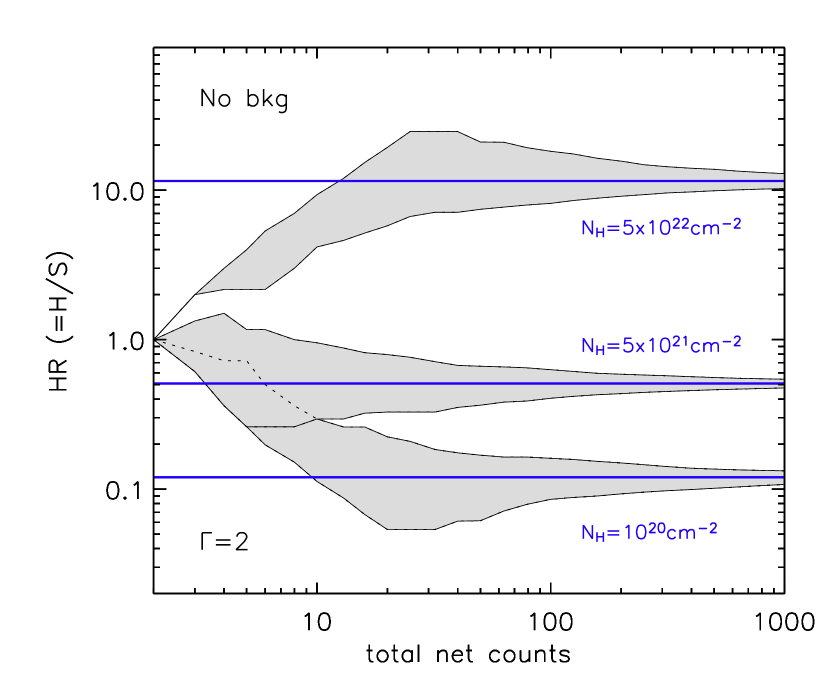
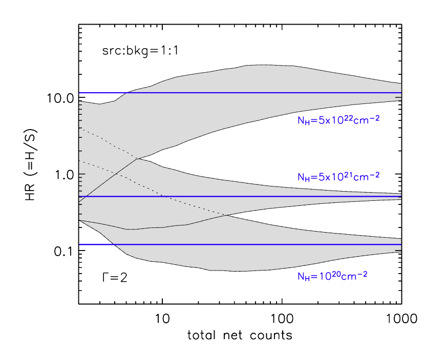
Figure 5: Conventional hardness ratio calculation. The soft band ($S$) is 0.3-2.0 keV and hard band ($H$) 2.0-8.0 keV, and the Chandra ACIS-S response function is used. The left two panels show a conventional hardness distribution as a function of total net counts and the right two panels show the fraction of the simulations that have $H>0$ and $S>0$ for a given total net count. The top two panels are for the case of no background, and in the bottom two panels, for a given net count, the source region contains an equal number of source and background counts, and we perform a background subtraction identical to the one described in the previous examples. Three spectral shapes ($\Gamma$ = 2) are simulated, and the solid horizontal lines in the left panels represent the true hardness ratio of each spectrum. The shaded region represents the central 68% of simulated results (only for $H>0$ and $S>0$) at a given total net count. A large fraction of trials do not produce a proper hardness ratio when the total counts are less than 100. Below 10 counts, the hardness distribution hardly bears any relation to its true value. Blending of the central 68% distributions starts at $\sim$ 40 counts for $N\mbox{$\rm{}_{H}$}$ = $10^{20}$ and $5\times 10^{21}$ cm^-2 for the case with background.

Fig. 6 shows the performance of the new hardness defined by the median. First, there is no loss of events. Second, three spectra are well separated down to less than 10 counts regardless of background. Even at two or three net counts, each distribution is distinct and well related to its true value.

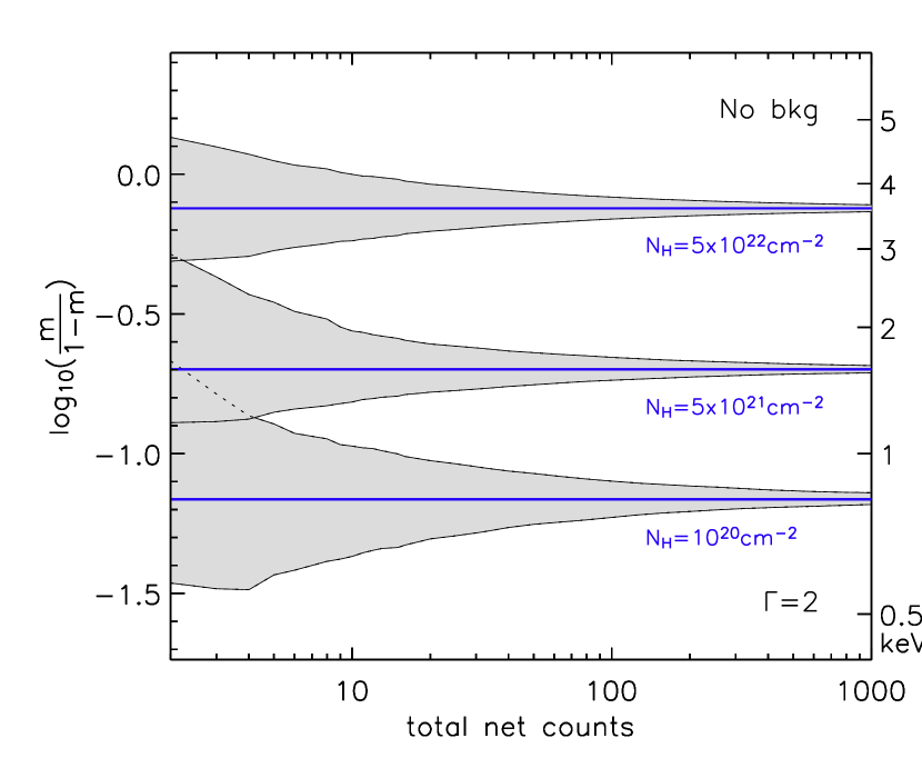
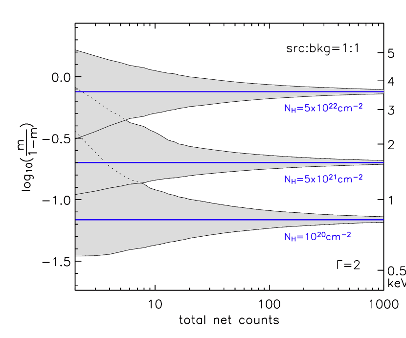
Figure 6: The median distribution for three power-law spectra with $\Gamma=2$. Compare this with Fig. 5. Regardless of background, the three distributions are well separated down to less than 10 counts, bearing a tight relation with their true value. In addition, there is no loss of events in this diagram.

5 Discussion

The newly defined hardness and color-color diagrams using the median and other quantiles are far superior to the conventional ones. One can choose specific quantiles and their combinations relevant to one’s needs. We believe the new phase space by the median and quartiles is very useful in general, as summarized in Fig. 7.

For a given spectrum, various quantiles are not independent variables, unlike the counts in different energy bands. However, the ratio of two quartiles is mostly independent from the median, which makes them good candidate parameters for color-color diagrams. In essence, the median $Q_{50}$ shows how dense the first (or second) half of the spectrum is and the quartile ratio $Q_{25}$/$Q_{75}$ shows a similar measure of the middle half of the spectrum.

For the $x$-axis in Fig. 7, one can simply use $m$ ($\equiv\mbox{$Q_{50}$}$) on a log scale to explore the wide range of the hardness. However, a simple log scale compresses the phase space for relatively hard spectra ($m>0.5$; note $0\leq m\leq 1$). Our expression, log($m/(1-m)$), shows both the soft and hard phase space equally well.

In Fig. 7, a flat spectrum lies at $x$=0 and $y$=1 in the diagram ($0<y<3$). The spectrum changes from soft to hard as one goes from left to right in the diagram, and it changes from concave-upwards to concave-downwards, as one goes from bottom to top. The examples in the previous sections explore a soft part of this phase diagram, which is modeled by a power law.

In the case of a narrow energy range, where an emission or absorption line is expected on a relatively flat continuum, one can use the QCCD to explore a spectral line feature even with limited statistics that normally forbids normal spectral fitting. In this case, the median ($x$-axis) in the QCCD can be a good measure of line shift, and the quartile ratio ($y$-axis) can be a good measure of line broadening.

The right panel in Fig. 7 shows the overlay of the grid patterns for typical spectral models - power law, thermal Bremsstrahlung, and black body emission. For high count sources, one can use such a diagram to find relevant models for the spectra before detailed analysis.

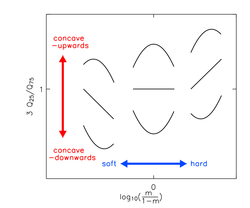
Figure 7: Overview of various spectral shapes (approximated as concave or straight lines) in the QCCD using $Q_{50}$ and $Q_{25}$/$Q_{75}$ (left), and the grid patterns for power law (PL), thermal Bremsstrahlung (TB), black body (BB) models in a 0.3-8.0 keV range ideal detector or incoming flux space (right). For PL, the grid patterns are for $\Gamma$ = 4, 3, 2, 1 & 0 along the positive $x$-axis direction, for TB, $kT$ = 0.2, 0.5, 1, 2, 4, & 10.0 keV, and for BB, $kT$ = 0.1, 0.2, 0.5, 1, 2, & 4 keV. For all the models, $N\mbox{$\rm{}_{H}$}$ = 0.1, 1, 5, & 10 $\times 10^{21}$ cm^-2 along the positive $y$ direction.

Finally, we investigate how the detector energy resolution affects the performance of the quantile-based diagram. The left panel in Fig. 8 shows the grid patterns of the power-law emission models for detectors with various energy resolutions but with the same detection efficiency of the Chandra ACIS-S detector. Starting with the energy resolution of the Chandra ACIS-S detector in the previous examples (Figs. 3, 4, 5 and 6; FWHM $\Delta E$ $\sim$ 150 eV at 1.5 keV and $\sim$ 200 eV at 4.5 keV), we have successively decreased the energy resolution by multiplying the energy resolution at each energy by a constant factor. Each pattern is labeled by the energy resolution ($\Delta E/E$) at 1.5 keV. As the energy resolution decreases, the grid pattern shrinks. The pattern will shrink down to a point ($x,y$)=(0,1) in the diagram for a detector with no energy resolution.

The right panel in Fig. 8 shows the 68% of the simulation results for a detector with $\Delta E/E$ = 100% at 1.5 keV. The size of the 68% distribution in this example is more or less similar to that in the case of the regular Chandra ACIS-S detector with $\Delta E/E$ = 10% (the top-right panel in the Fig. 3). The similarity is due to the fact that, unlike the grid pattern, the dispersion of the simulation results (or the error size of a data model point) for each model is mainly due to statistical fluctuations for low count sources. In summary, as the energy resolution decreases, the relative distance between various models in the diagram decreases, but the error size of the data remains roughly the same, and thus the spectral sensitivity of the diagram decreases.

Note that the overall size of the grid patterns in the left panel of Fig. 8 is more or less similar when $\Delta E/E\lesssim 20$% (at 1.5 keV). We expect that for a detector with energy resolution $\Delta E$, the overall size is dependent on a quantity $\Delta E/(E\mbox{$\rm{}_{up}$}-E\mbox{$\rm{}_{lo}$})$ since quantiles are determined over the full energy range. Therefore, the quantile-based diagram is quite robust against finite energy resolutions of typical X-ray detectors.

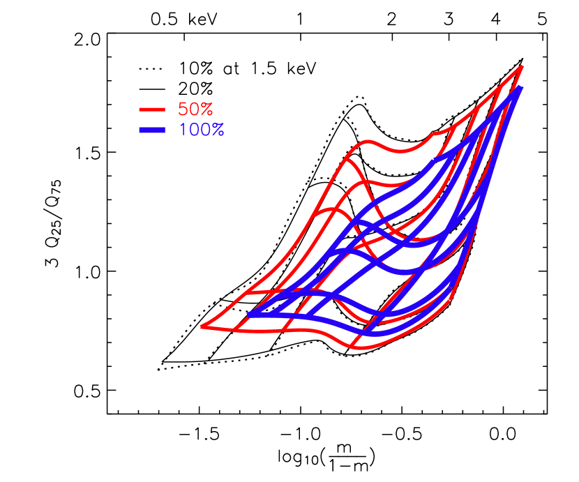
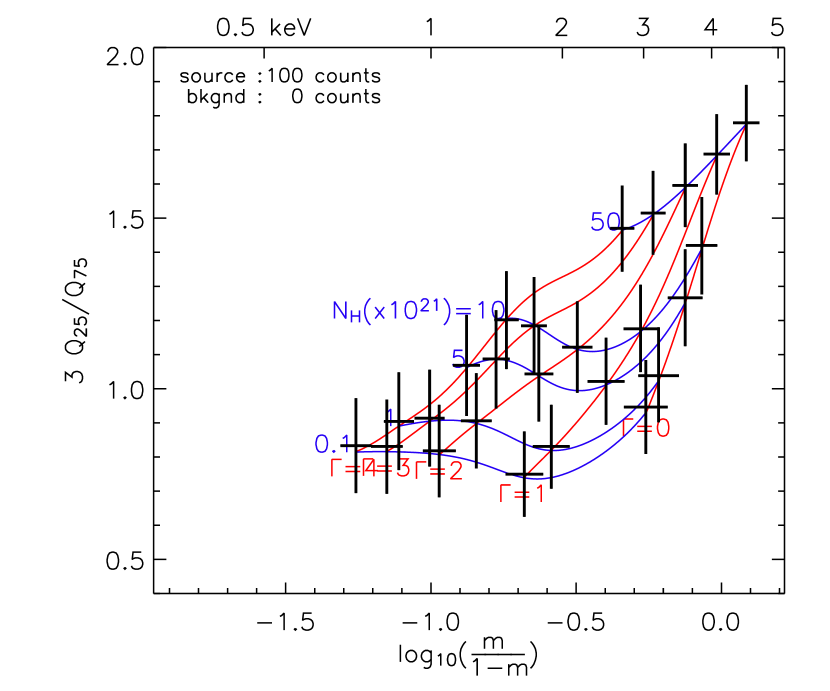
Figure 8: The grid patterns for various energy resolutions with the same Chandra ACIS-S efficiency (left) and the 68% distribution of the simulation results for 100 count sources for a detector with $\Delta E/E$ = 100% ($\Delta E=$FWHM) at 1.5 keV (right). Each grid pattern in the left panel is generated for a different energy resolution, labeled by the energy resolution ($\Delta E/E$) at 1.5 keV. As the resolution decreases, the pattern shrinks, and if there is no energy resolution in the detector, the pattern shrinks to a point at ($x,y$) = (0,1). The right figure shows the effects of limited photon statistics dominate those of energy resolution (compare with Fig. 3, with $\Delta E/E=$10% at 1.5 keV) in determining the 68% error bar sizes. See the electronic ApJ for color version of the figure which distiguished the model grids more easily.

Figure 9: Accuracy of the error estimates by the Maritz-Jarrett method: the ratio of the error estimate by the Maritz-Jarrett method ($\sigma$_mj) to that from simulations ($\sigma$_sim, the 68% distribution) for the cases with no background (left) and for the cases with high background (right). See the “background subtraction” section in the appendix for the background subtraction routine.

6 Acknowledgement

This work is supported by NASA grant AR4-5003A for our on-going Chandra Multiwavelength plane (ChaMPlane) survey of the galactic plane.

Many routines have been developed to estimate quantiles and the related statistics (Wilcox, 1997). We use a simple interpolation technique based on order statistics to estimate quantiles. For real data, we also need to have a reliable estimate for the errors of quantile values, for which we employ the technique by Maritz & Jarrett (1978). For simplicity, we assume that we measure the energy value of each photon.

Appendix A Quantile estimation using order statistics

In the literature, many quantile estimation algorithms often assume that the lowest value (energy) of the given distribution is the (equivalent) lower bound of the distribution and the highest value the upper bound. In X-ray astronomy, the lower ($E$_lo) and upper bound ($E$_up) of the energy range is usually set by the instrument or user selection, where these bounds may or may not be the lowest and highest energies of the detected photons. We can explicitly impose this boundary condition by assigning 0% and 100% quantiles to $E$_lo and $E$_up respectively.

We sort the detected photons in ascending order of energy, and we assign $E_{x\%}$ to the energy $E_{i}$ of the $i$-th photon as

$$E_{i} = E_{x\%},\text{\ where \ }\frac{x}{100}=\frac{2i-1}{2N},$$

and $N$ is the total number of net counts. Using $E$_lo=$E_{0\%}$ and $E$_up=$E_{100\%}$, one can interpolate any quantiles from the above relation of $x$ and $E_{i}$. With the definitions of $E$_lo=$E_{0\%}$ and $E$_up=$E_{100\%}$, the above interpolation is very robust. One can even calculate quantiles without any detected photons (although not meaningful), the result of which is identical to the case of a flat spectrum. In the case of only one detected photon at $E$, the above relation reduces to $E$=$E_{50\%}$. Therefore, the distribution of the median from one count sources with the same spectra is the source spectrum itself.

The above interpolation for quantile $E_{x\%}$ essentially uses only two energy values, $E_{i}$ and $E_{i+1}$, where $(2i-1)/2N<x/100<(2i+1)/2N$. In order to take advantage of other energy values, one can use more sophisticated techniques like that of Harrell & Davis (1982). In many cases, the Harrell-Davis method estimates quantiles with smaller uncertainties than the simple order statistics technique, but because of smoothing effects in the Harrell-Davis method, there are cases that the simple order statistics performs better, such as distributions containing discontinuous breaks (Wilcox, 1997). In real data, the finite detector resolution tends to smooth out any discontinuity in the spectra. Our simulation shows that about 10-15% better performance is achieved by the Harrell-Davis method compared to the simple order statistics for the cases of 50 source photons and 25 background photons. The results in the paper are generated by the order statistics technique.

Appendix B Quantile error estimation using the Maritz-Jarrett method

Once quantile values are acquired, one can always rely on simulations to estimate their uncertainty (or error) using a suspected spectral model with parameters derived from the QCCD. If no single model stands out as a primary candidate, one can derive a final uncertainty of the quantiles by combining the results of multiple simulations from a number of models. However, error estimation by simulations can be slow, cumbersome, and even redundant, considering that the quantile errors are more sensitive to the number of counts than the choice of spectral shapes (cf. Figs. 3 and 4). A quick and rough error estimate is often sufficient, and so we introduce a simple quantile error estimate technique – the Maritz-Jarrett method. The results (error bars and shades in Fig. 1 to 6) in the main text indicate the interval that encloses the central 68% of the simulation results, and were not driven by the Maritz-Jarrett method.

The Maritz-Jarrett method uses a technique similar to the Harrell-Davis method of quantile estimation. Both methods rely on L-estimators (linear sums of order statistics) using Beta functions. We sort the photons in the ascending order of energy from $i=1$ to $N$. Then, we apply the Maritz-Jarrett method with small modifications as follows. For $E_{x\%}$, we set

$$M = Nx+0.5$$

$$a = M-1$$

$$b = N-M.$$

We then define $W_{i}$ using the incomplete beta function $B$,

$$W_{i} = B(a,b,y_{i+1})-B(a,b,y_{i})$$

$$B(a,b,y) = \frac{\Gamma(a+b)}{\Gamma(a)\Gamma(b)}\int_{0}^{y}t^{a-1}(1-t)^{b-1}dt$$

where $y_{i}=i/N$ and $\Gamma(n+1)=n!$ (the gamma function). Using $W_{i}$ and $E_{i}$, we calculate the L-estimators $C_{k}$,

$$C_{k} = \sum^{N}_{i=1}W_{i}E_{i}^{k},\text{\ and then}$$

$$\sigma(E_{x\%}) = \sqrt{C_{2}-C^{2}_{1}}.$$

The error estimate by the Maritz-Jarrett method requires at least 3 counts for medians, 5 counts for terciles, and 6 counts for quartiles ($a,b\geq 1$) .

Fig. 9 shows the accuracy of the error estimates by the Maritz-Jarrett method for $\Gamma$ = 2 and $\mbox{$N\mbox{$\rm{}_{H}$}$}=5\times 10^{21}$ cm^-2. In the case of no background, the Maritz-Jarrett method is accurate when the total net counts are greater than $\sim$ 30. It tends to overestimate the errors when the total net counts are below $\sim$ 30. In the case of high background, it tends to underestimate the errors overall since the adopted background subtraction procedure (see below) does not inherit background statistics for the error estimates. We find that multiplying by an empirical factor $\sqrt{1+N\mbox{$\rm{}_{bkg}$}/N\mbox{$\rm{}_{src}$}}$ can compensate, approximately, for the underestimation ($N\mbox{$\rm{}_{src}$}$: total source counts, $N\mbox{$\rm{}_{bkg}$}$: total background counts).

For the error of the ratio $Q_{25}$/$Q_{75}$, since these two quartiles are not independent variables, the simple quadratic combination from two quartile errors overestimates the error of the ratio ($\sim$ 20 – 30% for the examples in Figs. 3 and 4). One can find more sophisticated techniques such as Bayesian statistics to estimate quantile errors in the literature. For example, Babu (1999) and the reference therein discuss the limitation of bootstrap estimation and show other techniques such as the half-sample method.

Appendix C Background Subtraction

For background subtraction, we calculate quantiles at a set of finely stepped fractions separately for photons in the source region and the background region. Then, by a simple linear interpolation, we establish the integrated counts $IC(>$$E)$ (number of photons with energy greater than $E$) as a function of energy for both regions. Now at each energy, one can subtract the integrated counts of the background region from that of the source region with a proper ratio factor of the area of the two regions. Because of statistical fluctuations, the subtracted integrated net counts may not be monotonically increasing from $E\mbox{$\rm{}_{lo}$}$ to $E\mbox{$\rm{}_{up}$}$. Therefore we force a monotonic behavior by setting $IC(>$$E)\geq IC(>$$E^{\prime})$ if $IC(>$$E)<IC(>$$E^{\prime})$ and $E>E^{\prime}$. Such a requirement can underestimate the quantiles overall, so we repeat the above using $IC(<$$E)$ and force a monotonic decrease. Then, quantiles for the net distribution are given by

$$x = \frac{N+\mbox{$IC(>$$E)$}-\mbox{$IC(<$$E)$}}{2N}$$

$$E_{x\%} = E$$

where $N$ is the total net counts. If there is no statistical fluctuation, $IC(>$$E)=N-IC(<$$E)$. For the error estimation, we need to know the energy of each source photon, which will be lost from background subtraction. So we generate a set of $N$ energy values for source photons matching the above quantile relation and then apply the above error estimation technique using the Maritz-Jarrett method.

References

- Babu (1999) Babu, G. J. 1999 ”Breakdown theory for estimators based on bootstrap and other resampling schemes” in Asymptotics, Nonparameterics, and Time Series (eg. S. Ghosh), Stat. Text. Monogr. 158, Dekker:NY, pp 669-681.
- Harrell & Davis (1982) Harrell, F. E. & Davis, C. E., 1982, Biometrika, 69, 635-640
- Kim et al. (1992) Kim, D. W., Fabbiano, G., & Trinchieri, G. 1992, ApJ, 393, 134
- Kim et al. (2003) Kim, D. W., et al., 2003 ApJ, in press (astro-ph/0308493)
- Maritz & Jarrett (1978) Maritz, J. S. & Jarrett, R. G., 1978, Journal of the American Statistical Association, 73, 194-196
- Netzer et al. (1994) Netzer, H., Turner, T. J., George, I. M. 1994, ApJ, 435, 106
- Prestwich et al. (2003) Prestwich, A. H., Irwin, J. A., Kilgard, R. E., Krauss, M. I.; Zezas, A., Primini, F., Kaaret, P., Boroson, B. 2003, ApJ, 595, 719
- e.g. Schulz et al. (1989) Schulz, N. S., Hasinger, G., & Trumper, J. 1989, A&A, 225, 48
- Wilcox (1997) Wilcox, R. R., Introduction to Robust Estimation and Hypothesis Testing, Academic Press, 1997