Analysis of the Spatial Distribution of Galaxies by Multiscale Methods

Abstract

Galaxies are arranged in interconnected walls and filaments forming a cosmic web encompassing huge, nearly empty, regions between the structures. Many statistical methods have been proposed in the past in order to describe the galaxy distribution and discriminate the different cosmological models. We present in this paper results relative to the use of new statistical tools using the 3D isotropic undecimated wavelet transform, the 3D ridgelet transform and the 3D beamlet transform. We show that such multiscale methods produce a new way to measure in a coherent and statistically reliable way the degree of clustering, filamentarity, sheetedness, and voidedness of a dataset.

1 Introduction

Galaxies are not uniformly distributed throughout the universe. Voids, filaments, clusters, and walls of galaxies can be observed, and their distribution constraints our cosmological theories. Therefore we need reliable statistical methods to compare the observed galaxy distribution with theoretical models and cosmological simulations.

The standard approach for testing models is to define a point process which can be characterized by statistical descriptors. This could be the distribution of galaxies of a specific type in deep redshift surveys of galaxies (or of clusters of galaxies). In order to compare models of structure formation, the different distribution of dark matter particles in N-body simulations could be analyzed as well, with the same statistics.

The two-point correlation function $\xi(r)$ has been the primary tool for quantifying large-scale cosmic structure [24]. Assuming that the galaxy distribution in the Universe is a realization of a stationary and isotropic random process, the two-point correlation function can be defined from the probability $\delta P$ of finding an object within a volume element $\delta V$ at distance $r$ from a randomly chosen object or position inside the volume: $\delta P=n(1+\xi(r))\delta V$, where $n$ is the mean density of objects. The function $\xi(r)$ measures the clustering properties of objects in a given volume. It is zero for a uniform random distribution, positive (respectively, negative) for a more (respectively, less) clustered distribution. For a hierarchical clustering or fractal process, $1+\xi(r)$ follows a power-law behavior with exponent $D_{2}-3$. Since $\xi(r)\sim r^{-\gamma}$ for the observed galaxy distribution, the correlation dimension for the range where $\xi(r)\gg 1$ is $D_{2}\simeq 3-\gamma$. The Fourier transform of the correlation function is the power spectrum. The direct measurement of the power spectrum from redshift surveys is of major interest because model predictions are made in terms of the power spectral density. It seems clear that the real space power spectrum departs from a single power-law ruling out simple unbounded fractal models [36]. The two-point correlation function can been generalized to the N-point correlation function [35, 25], and all the hierarchy can be related with the physics responsible for the clustering of matter. Nevertheless they are difficult to measure, and therefore other related statistical measures have been introduced as a complement in the statistical description of the spatial distribution of galaxies [20], such as the void probability function [21], the multifractal approach [18], the minimal spanning tree [1, 15, 8], the Minkowski functionals [22, 13] or the $J$ function [17, 14] which is defined as the ratio $J(r)=\frac{1-G(r)}{1-F(r)}$, where $F$ is the distribution function of the distance $r$ of an arbitrary point in ${\bf R}^{3}$ to the nearest object in the catalog, and $G$ is the distribution function of the distance $r$ of an object to the nearest object. Wavelets have also been used for analyzing the projected 2D or the 3D galaxy distribution [9, 28, 19, 23, 16].

The Genus statistic [10] measures the topology or the degree of connectedness of the underlying density field. Phase correlations of the density field can be detected by means of this topological analysis. The Genus is calculated by (i) convolving the data by a kernel, generally a Gaussian, (ii) setting to zero all values under a threshold $\nu$ in the obtained distribution, and (iii) taking the difference $D$ between the number of holes and the number of isolated regions. The Genus curve $G(\nu)$ is obtained by varying the threshold level $\nu$. The first step of the algorithm, the convolution by a Gaussian, may be dramatic for the description of filaments, which are spread out along all directions, as it will be shown in next section. The Genus is related with one of the four Minkowski functionals that describe well the overall morphology of the galaxy distribution [26]. Minkowski functionals have been used to elaborate sophisticated tools to measure the filamentarity and planarity of the distribution by means of shape finders quantities [27].

The Sloan Digital Sky Survey (Early Data Release) has recently be analyzed using a 3D Genus Statistics [11] and results were consistent with that predicted by simulations of a $\Lambda$-dominated spatially-flat cold dark matter model.

New multiscale methods have recently emerged, the beamlet transform [4, 6] and the ridgelet transform [3], which allows us to better represent data containing respectively filaments and sheets, while wavelets represent well isotropic features (i.e. cluster in 3D). As each of these three transforms represents perfectly one kind of feature, all of them are useful and should be used to describe a given catalog.

Section 2 describes the 3D wavelet transform, and how wavelets can be used for estimating the underlying density. Sections 3 and 4 describes respectively the 3D ridgelet transform and the 3D beamlet transform. It is shown in section 4 through a set of of experiments how these three 3D transforms can be combined in order to describe statistically the distribution of galaxies.

2 The 3D Wavelet Transform

2.1 The Undecimated Isotropic Wavelet Transform

The wavelet transform of a signal produces, at each scale $j$, a set of zero-mean coefficient values $\{w_{j}\}$. Using an algorithm such as the undecimated isotropic wavelet decomposition [33], this set $\{w_{j}\}$ has the same number of pixels as the signal and thus this wavelet transform is a redundant one. Furthermore, using a wavelet defined as the difference between the scaling functions of two successive scales

$$\frac{1}{8}\psi(\frac{x}{2},\frac{y}{2},\frac{z}{2})=\phi(x,y,z)-\frac{1}{8}\phi(\frac{x}{2},\frac{y}{2},\frac{z}{2}),$$ (1)

the original cube $c=c_{0}$ can be expressed as the sum of all the wavelet scales and the smoothed array $c_{J}$

$$c_{0,x,y,z}=c_{J,x,y,z}+\sum_{j=1}^{J}w_{j,x,y,z}\ ,$$ (2)

The set $w=\{w_{1},w_{2},...,w_{J},c_{J}\}$, where $c_{J}$ is a last smooth array, represents the wavelet transform of the data. If we denote as ${\cal W}$ the wavelet transform operator and $N$ the pixel number of $c$, the wavelet transform $w$ ($w={\cal W}c$) has $(J+1)N$ pixels (redundancy factor of $J+1$). The scaling function $\phi$ is generally chosen as a spline of degree 3, and the 3D implementation is based on three 1D sets of (separable) convolutions. Like the scaling function $\phi$, the wavelet function $\psi$ is isotropic (point symmetric). More details can be found in [33, 32].

For each $a>0$, $b_{1},b_{2},b_{3}\in{\bf R}^{3}$ , the wavelet is defined by

$\begin{array}[]{ll}\psi_{a,b_{1},b_{2},b_{3}}:&{\bf R}^{3}\rightarrow{\bf R}\\ &\psi_{a,b_{1},b_{2},b_{3}}(x_{1},x_{2},x_{3})=a^{-1/2}\cdot\psi(\frac{x_{1}-b_{1}}{a},\frac{x_{2}-b_{2}}{a},\frac{x_{3}-b_{3}}{a})\end{array}$

Given a function $f\in L^{2}({\bf R}^{3})$, we define its wavelet coefficients by:

$\begin{array}[]{lll}\mathcal{W}_{f}:&{\bf R}^{4}\rightarrow{\bf R}\\ &\mathcal{W}_{f}(a,b_{1},b_{2},b_{3})=\int\overline{\psi}_{a,b_{1},b_{2},b_{3}}(\mathbf{x})f(\mathbf{x})d\mathbf{x}.\end{array}$

Figure 1: Example of wavelet function.

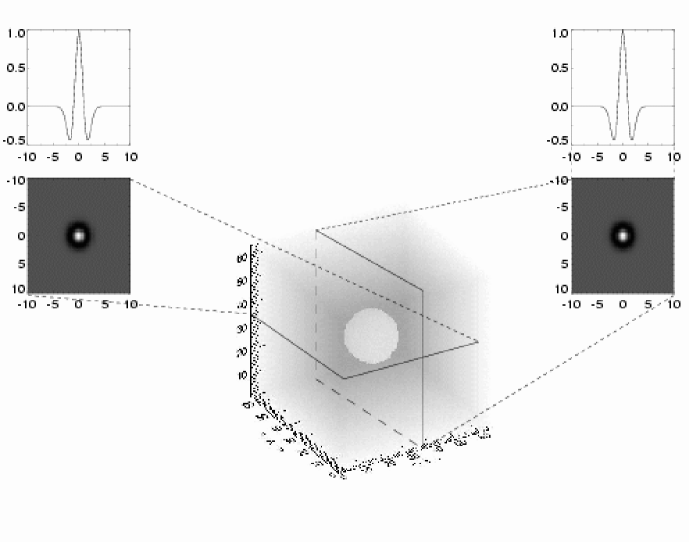
Figure 1 shows an example of 3D wavelet function.

2.2 3D Galaxy Distribution Filtering

For the noise model, given that this relates to point pattern clustering, we have to consider the Poisson noise case. The autoconvolution histogram method used for X-ray image [34] can also be used here. It consists to calculate numerically the probability distribution function (pdf) of a wavelet $w_{j,x,y,z}$ coefficient with the hypothesis that the galaxies used for obtaining $w_{j,x,y,z}$ are randomly distributed. The pdf is obtained by autoconvolving $n$ times the histogram of the wavelet function, $n$ being the number of galaxies which have been used for obtaining $w_{j,x,y,z}$, i.e. the number of galaxies in a box around $(x,y,x)$, the size of the box depending of the scale $j$. More details can be found in [34, 32].

Once the pdf relative to the coefficient $w_{j,x,y,z}$ is known, we can detect the significant wavelet coefficients easily. We derive two threshold values $T^{min}_{j,x,y,z}$ and $T^{max}_{j,x,y,z}$ such that

$$Prob(W<T^{min}_{j,x,y,z}) = \epsilon$$

$$Prob(W>T^{max}_{j,x,y,z}) = \epsilon$$ (3)

$\epsilon$ corresponding to the confidence level, and the positive (respective negative) wavelet coefficient is significant if it is larger than $T^{max}_{j,x,y,z}$ (resp. lower than $T^{min}_{j,x,y,z}$).

A simple filtering method would now consist to set to zero (i.e. thresholding) all unsignificant coefficients and reconstruct the filtered data cube by addition of the different scales. But when a redundant wavelet transform is used, the result after a simple hard thresholding can still be improved by iterating [30]. We want the wavelet transform of our solution $\tilde{s}$ to reproduce the same significant wavelet coefficients (i.e., coefficients larger than $T_{j}$). This can be expressed in the following way:

$$({\cal W}\tilde{s})_{j,k}=w_{j,k}\mbox{ if }w_{j,k}\mbox{ is significant }$$ (4)

where $w_{j,k}$ are the wavelet coefficients of the input data $s$ at scale $j$ and at position $k=(x,y,z)$. The relation is not necessarily verified in the case of non-orthogonal transforms, and the resulting effect is generally a loss of flux inside the objects. The residual signal (i.e. $s-\tilde{s}$) still contains some information at positions where the objects are.

Denoting $M$ the multiresolution support of $s$ (i.e. $M_{j,k}=1$ if $w_{j,k}$ is significant, and 0 otherwise), we want:

$$M.{\cal W}\tilde{s}=M.{\cal W}s$$

The solution can be obtained by the following Van Cittert iteration [33]:

$$\tilde{s}^{n+1} = \tilde{s}^{n}+{\cal W}^{-1}(M.{\cal W}s-M.{\cal W}s^{n})$$ (5)

$$= \tilde{s}^{n}+{\cal W}^{-1}(M.{\cal W}R^{n})$$

where $R^{n}=s-\tilde{s}^{n}$.

Iterative Filtering with a Smoothness Constraint

A smoothness constraint can be imposed on the solution.

$$\min\|{\cal W}\tilde{s}\|_{\ell_{1}},\quad\mbox{subject to}\quad s\in C,$$ (6)

where $C$ is the set of vectors $\tilde{s}$ which obey the linear constraints

$$\left\{\begin{array}[]{ll}\tilde{s}_{k}\geq 0,\forall k\\ \mid({\cal W}\tilde{s}-{\cal W}s)_{j,k}\mid\leq e_{j};\end{array}\right.$$ (7)

Here, the second inequality constraint only concerns the set of significant coefficients, i.e. those indices which exceed (in absolute value) a detection threshold $t_{j}$. Given a tolerance vector $e=\{e_{1},...,e_{j}\}$, we seek a solution whose coefficients $({\cal W}\tilde{s})_{j,k}$, at scale and position where significant coefficients were detected, are within $e_{j}$ of the noisy coefficients $({\cal W}s)_{j,k}$. For example, we can choose $e_{j}=\sigma_{j}/2$. In short, our constraint guarantees that the reconstruction be smooth but will take into account any pattern which is detected as significant by the wavelet transform.

We use an $\ell_{1}$ penalty on the coefficient sequence because we are interested in low complexity reconstructions. There are other possible choices of complexity penalties; for instance, an alternative to (6) would be

$$\min\|\tilde{s}\|_{TV},\quad\mbox{subject to}\quad s\in C.$$

where $\|\cdot\|_{TV}$ is the Total Variation norm, i.e. the discrete equivalent of the integral of the Euclidean norm of the gradient. Expression (6) can be solved using the method of hybrid steepest descent (HSD) [38]. HSD consists of building the sequence

$$\tilde{s}^{n+1}=P(\tilde{s}^{n})-\lambda_{n+1}\nabla_{J}(P(\tilde{s}^{n}));$$ (8)

here, $P$ is the $\ell_{2}$ projection operator onto the feasible set $C$, $\nabla_{J}$ is the gradient of equation (6), and $(\lambda_{n})_{n\geq 1}$ is a sequence obeying $(\lambda_{n})_{n\geq 1}\in[0,1]$ and $\lim_{n\rightarrow+\infty}\lambda_{n}=0$.

Unfortunately, the projection operator $P$ is not easily determined and in practice we use the following proxy; compute ${\cal W}\tilde{s}$ and replace those coefficients which do not obey the constraints $|({\cal W}\tilde{s}-{\cal W}s)_{j,k}|\leq e_{j}$ (those which fall outside of the prescribed interval) by those of $s$; apply the inverse transform.

The filtering algorithm is:

1. Initialize $L_{\max}=1$, the number of iterations $N_{i}$, and $\delta_{\lambda}=\frac{L_{\max}}{N_{i}}$.

2. Estimate the noise standard deviation $\sigma_{s}$, and set $e_{j}={\sigma_{j}\over 2}$ for all $j$.

3. Calculate the transform: $w^{(s)}={\cal W}s$.

4. Set $\lambda=L_{\max}$, $n=0$, and $\tilde{s}^{n}$ to 0.

5. While $\lambda>=0$ do

   • $u=\tilde{s}^{n}$.

     • Calculate the transform $\alpha={\cal W}u$.

     • For all coefficients $\alpha_{j,k}$ do

       • Calculate the residual $r_{j,k}=w^{(s)}_{j,k}-\alpha_{j,k}$

       • if $w^{(s)}_{j,k}$ is significant and $\mid r_{j,k}\mid\ >e_{j}$ then $\alpha_{j,k}=w^{(s)}_{j,k}$

       • $\alpha_{j,k}=sgn(\alpha_{j,k})(\mid\alpha_{j,k}\mid-\lambda\sigma_{j})_{+}$.

     • $u={{\cal W}}^{-1}\alpha$

   • Threshold negative values in $u$ and $\tilde{s}^{n+1}=u$.

   • $n=n+1$, $\lambda=\lambda-\delta_{\lambda}$, and goto 5.

In practice, a small number of iterations ($<$10) is enough. The $(.)_{+}$ operator means that negative values are set to zero ($(a)_{+}=\mbox{MAX}(0,a)$).

Experiments

Figure 2: Simulated data.

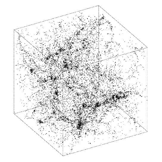
Fig. 2 shows a simulation of a $60h^{-1}$ Mpc box of universe, made by A. Klypin (simulated data at http://astro.nmsu.edu/$\sim$aklypin/PM/pmcode). It represents the distribution of dark matter in the present-day universe and each point is a dark matter halo where visible galaxies are expected to be located, i.e. the distribution of dark matter halos can be compared with the distribution of galaxies in catalogs of galaxies.

Figure 3: Simulated data filtered by a Gaussian filter (two left panels corresponding respectively to $\sigma=1$ and $\sigma=3$) and using the wavelet algorithm described in the text (right panel).

Figure 4: The genus curve for the N-body model shown in Fig. 2 convolving the data with a Gaussian filter with different values of $\sigma$ and the genus for the wavelet filtered data set.

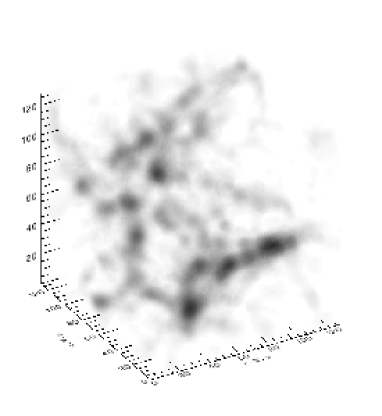
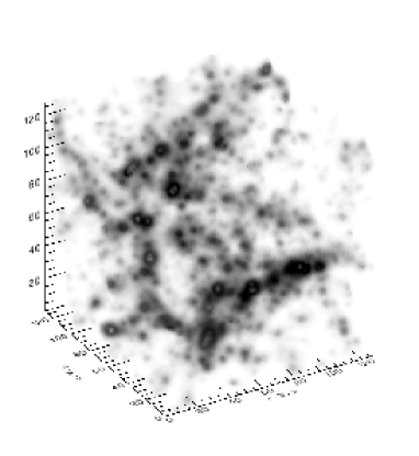
Fig. 4 shows, at the right panel, the same data set filtered by the 3D wavelet transform, using the algorithm described previously. The two left panels correspond to Gaussian smoothing

$$W({\bf x})=\frac{1}{(2\pi)^{3/2}\sigma^{3}}\exp\left(-\frac{{\bf x}^{2}}{2\sigma^{2}}\right).$$ (9)

with $\sigma=1$ and $\sigma=3$. We can see that when the bandwidth is too small the discreteness and the noise dominate the density reconstructed field, while large value of $\sigma$ erase all the small scale features of the distribution. This is illustrated in Fig. 4, where we can see the strong dependence of the genus curve with the width of the Gaussian filter, being its interpretation completely dependent of the choice of the bandwidth. The wavelet reconstructed density field keeps information at all scales due to its multiscale nature. This is observed in the 3D image at the right panel of Fig. 4, where we see how large filaments, big clusters and walls coexist with small scale features such as the density enhancement around groups and small clusters. The genus curve of this adaptive reconstructed density field is much more informative because it does not depend of the particular choice of the filter radius.

3 The 3D Ridgelet Transform

3.1 The 2D Ridgelet Transform

The two-dimensional continuous ridgelet transform of a function $f\in L^{2}({\bf R}^{2})$ is defined as follows [3].
We first select a smooth function $\psi\in L^{2}({\bf R})$, we assume that $\psi$ satisfies the admissibility condition

$$\int|\hat{\psi}(\xi)|^{2}/|\xi|\,d\xi<\infty,$$ (10)

which holds if $\psi$ has a sufficient decay and a vanishing mean $\int\psi(t)dt=0$ ($\psi$ can be normalized so that it has unit energy $1/(2\pi)\int|\hat{\psi}(\xi)|^{2}d\xi=1$).
For each $a>0$, $b\in{\bf R}$ and $\theta_{1}\in[0,2\pi[$, we define the ridgelet by

$\begin{array}[]{ll}\psi_{a,b,\theta_{1}}:&{\bf R}^{2}\rightarrow{\bf R}\\ &\psi_{a,b,\theta_{1}}(x_{1},x_{2})=a^{-1/2}\cdot\psi((x_{1}\cos\theta_{1}+x_{2}\sin\theta_{1}-b)/a);\end{array}$
Given a function $f\in L^{2}({\bf R}^{2})$, we define its ridgelet coefficients by:

$\begin{array}[]{lll}{\cal R}_{f}:&{\bf R}^{3}\rightarrow{\bf R}\\ &{\cal R}_{f}(a,b,\theta_{1})=\int\overline{\psi}_{a,b,\theta_{1}}(\mathbf{x})f(\mathbf{x})d\mathbf{x}.\end{array}$

Figure 5: Definition of angle1 $\theta_{1}$ and $\theta_{2}$ in ${\bf R}^{2}$ and ${\bf R}^{3}$

It has been shown [3] that the ridgelet transform is precisely the application of a 1-dimensional wavelet transform to the slices of the Radon transform (where the angular variable $\theta_{1}$ is constant). This method is therefore optimal to detect lines of the size of the image (the integration increase as the length of the line). More details on the implementation of the digital ridgelet transform can be found in [31].

Figure 6: Example of 2D ridgelet function.

Figure 6 (left) shows an example ridgelet function. This function is constant along lines $x_{1}\cos\theta+x_{2}\sin\theta=const$. Transverse to these ridges it is a wavelet (see figure 6 (right).

3.2 From 2D to 3D

The three-dimensional continuous ridgelet transform of a function $f\in L^{2}({\bf R}^{3})$ is given by:

$\begin{array}[]{lll}{\cal R}_{f}:&{\bf R}^{4}\rightarrow{\bf R}\\ &{\cal R}_{f}(a,b,\theta_{1},\theta_{2})=\int\overline{\psi}_{a,b,\theta_{1},\theta_{2}}(\mathbf{x})f(\mathbf{x})d\mathbf{x}.\end{array}$
where $a>0$, $b\in{\bf R}$ , $\theta_{1}\in[0,2\pi[$ and $\theta_{2}\in[0,\pi[$.
The ridgelet function is defined by:

$\begin{array}[]{ll}\psi_{a,b,\theta_{1},\theta_{2}}:&{\bf R}^{3}\rightarrow{\bf R}\\ &\psi_{a,b,\theta_{1},\theta_{2}}(x_{1},x_{2},x_{3})=a^{-1/2}\cdot\psi((x_{1}\cos\theta_{1}\cos\theta_{2}+x_{2}\sin\theta_{1}\cos\theta_{2}+x_{3}\sin\theta_{2}-b)/a);\end{array}$

Figure 7: Example of ridgelet function.

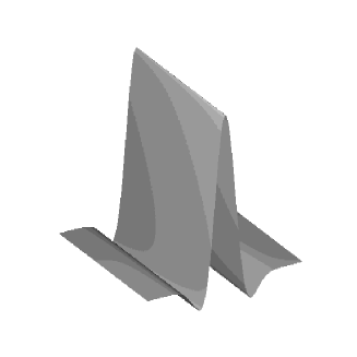
Figure 7 shows an example of ridgelet function. It is a wavelet function in the direction defined by the line $(\theta_{1},theta_{2})$, and it is constant along the orthogonal plane to this line.

Figure 8: 3D ridgelet transform flowgraph.

As in the 2D case, the 3D ridgelet transform can be built by extracting lines in the Fourier domain. Let $c(i_{1},i_{2},i_{3})$ a cube of size $(N,N,N)$, the algorithm consists in the following steps:

1. 3D-FFT. Compute $\hat{c}(k_{1},k_{2},k_{3})$, the three-dimensional FFT of the cube $c(i_{1},i_{2},i_{3})$.

2. Cartesian to Spherical Conversion. Using an interpolation scheme, substitute the sampled values of $\hat{c}$ obtained on the Cartesian coordinate system $(k_{1},k_{2},k_{3})$ with sampled values of on a spherical coordinate system $(\theta_{1},\theta_{2},\rho)$.

3. Extract lines. Extract the $3N^{2}$ lines (size $N$) passing through the origin and the boundary of $\hat{c}$.

4. 1D-IFFT. Compute the one-dimensional inverse FFT on each line.

5. 1D-WT. Compute the one-dimensional wavelet transform on each line.

Figure 8 the 3D ridgelet transform flowgraph. The 3D ridgelet transform allows us to detect sheets in a cube.

Local 3D Ridgelet Transform

The ridgelet transform is optimal to find sheets of the size of the cube. To detect smaller sheets, a partitioning must be introduced [2]. The cube $c$ is decomposed into blocks of lower side-length $b$ so that for a $N*N*N$ cube, we count $N/b$ blocks in each direction. After the block partitioning, The detection is therefore optimal for sheets of size $b\times b$ and of thickness $a_{j}$, $a_{j}$ corresponding to the different dyadic scales used in the transformation.

4 The 3D Beamlet Transform

4.1 Definition

The X-ray transform of a continuum function $f(x,y,z)$ with $(x,y,z)\in{\bf R}^{3}$ is defined by

$$(Xf)(L)=\int_{L}f(p)dp$$ (11)

where $L$ is a line in ${\bf R}^{3}$, and $p$ is a variable indexing points in the line. The transformation contains all line integrals of $f$. The Beamlet Transform (BT) can be seen as a multiscale digital X-ray transform. It is multiscale transform because, in addition to the multiorientation and multilocation line integral calculation, it integrated also over line segments at different length. The 3D BT is an extension to the 2D BT, proposed by Donoho and Huo [4].

The system of 3D beams

The first choice to consider is the line segment set. We would like to have an expressive set of line segments in the sense that it includes line segments with various lengths, locations and orientations lying inside a 3D volume and at the same time has reasonable size.

A seemingly natural candidate for the set of line segments is the family of all line segments between any voxel corner and any other voxel corner, the set of 3-D beams. The beams set is expressive but can be of huge cardinality for even moderate resolutions. For a 3D data set with $n^{3}$ voxels we get $O(n^{6})$ 3D beams - So that is clearly infeasible to use the collection of 3-D beams as a basic data structure since any algorithm based on this set will have a complexity with lower bound of $n^{6}$ and hence unworkable for typical sizes 3-D images.

4.2 The Beamlet System

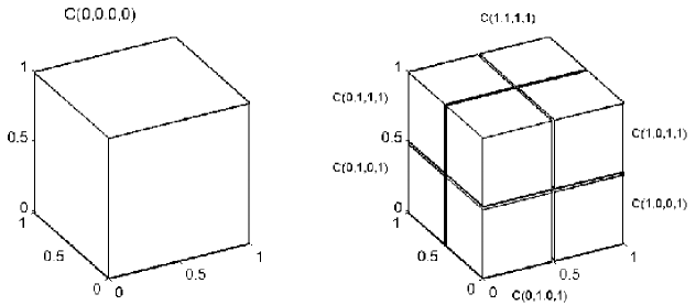
A dyadic cube $C(k_{1},k_{2},k_{3},j)\subset[0,1]^{3}$ is the collection of points

$$\{(x_{1},x_{2},x_{3}):[k_{1}/2^{j},(k_{1}+1)/2^{j}]\times[k_{2}/2^{j},(k_{2}+1)/2^{j}]\times[k_{3}/2^{j},(k_{3}+1)/2^{j}]\}$$

where $0\leq k_{1},k_{2},k_{3}<2^{j}$ for an integer $j\geq 0$. We will refer to $j$ as the scale of the dyadic cube

Such cubes can be viewed as descended from the unit cube $C(0,0,0,0)=[0,1]^{3}$ by recursive partitioning. Hence, the result of splitting $C(0,0,0,0)$ in half along each axis is the eight cubes $C(k_{1},k_{2},k_{3},1)$ where $k_{i}\in\{0,1\}$, splitting those in half along each axis we get the $64$ subcubes $C(k_{1},k_{2},k_{3},2)$ where $k_{i}\in\{0,1,2,3\}$, and if we decompose the unit cube into $n^{3}$ voxels using a uniform $n$-by-$n$-by-$n$ grid with $n=2^{J}$ dyadic, then the individual voxels are the $n^{3}$ cells $C(k_{1},k_{2},k_{3},J)$, $0\leq k_{1},k_{2},k_{3}<n.$

Figure 9: Dyadic cubes

Associated to each dyadic cube we can build a system of line segments that have both of their end-points lying on the cube boundary. We call each such segment A beamlet. If we consider all pairs of boundary voxel corners we get $O(n^{4})$ beamlets for a dyadic cube with a side length of $n$ voxels, we will work with a slightly different system in which each line is associated with a slope and an intercept instead of its end-points as will be explained below. However, we will still have $O(n^{4})$ cardinality. Assuming a voxel size of $1/n$ we get $J+1$ scales of dyadic cubes where $n=2^{J}$, for any scale $0\leq j\leq J$ there are $2^{3j}$ dyadic cubes of scale $j$ and since each dyadic cube at scale $j$ has a side length of $2^{J-j}$ voxels we get $O(2^{4(J-j)})$ beamlets associated with the dyadic cube and a total of $O(2^{4J-j})=O(n^{4}/2^{j})$ beamlets at scale j. If we sum the number of beamlets at all scales we get $O(n^{4})$ beamlets.

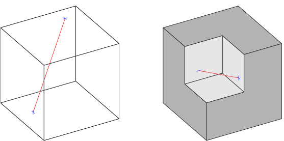
We have constructed above a multi-scale arrangement of line segments in 3D with controlled cardinality of $O(n^{4})$, the scale of a beamlet is defined as the scale of the dyadic cube it belongs to so lower scales correspond to longer line segments and finer scales correspond to shorter line segments. Figure 10 shows 2 beamlets at different scales.

Figure 10: Examples of Beamlets at two different scales. (a) Scale 0 (coarsest scale) (b) Scale 1 (next finer scale).

To construct the set of beamlets for a given dyadic cube we use the slope-intercept pairs system. For a data cube of $n\times n\times n$ voxels consider a coordinate system with the cube center of mass at the origin and a unit length for a voxel. Hence, for $(x,y,z)$ in the data cube we have $|x|,|y|,|z|\leq n/2$. We can consider three kinds of lines: $x$-driven, $y$-driven, and $z$-driven, depending on which axis provides the shallowest slopes. An $x$-driven line takes the form

$$z=s_{z}x+t_{z},\quad y=s_{y}x+t_{y}$$

with slopes $s_{z}$,$s_{y}$, and intercepts $t_{z}$ and $t_{y}$. Here the slopes $|s_{z}|,|s_{y}|\leq 1$. $y$- and $z$-driven lines are defined with an interchange of roles between $x$ and $y$ or $z$, as the case may be.

We will consider the family of lines generated by this, where the slopes and intercepts run through an equispaced family:

$$s_{x},s_{y},s_{z}\in\{2\ell/n:\ell=-n/2,\dots,n/2-1\},\qquad t_{x},t_{y},t_{z}\in\{\ell:-n/2,\dots,n/2-1\}.$$

Using the above family of lines for a given data cube we can define the set of beamlets belong to the cube to be the set of line segment obtained by taking the intersection of each line with the cube.

With the choice of indices range above we get that all beamlets associated with a data cube of size $n$ have lengths bigger than $n/2$, half of the cube length and $\sqrt{3}n$, the cube main diagonal length.

Computational aspects

The Beamlet coefficients are the line integrals over the set of beamlets. A digital 3-D image can be regarded as a 3-D piece-wise constant function and each line integral is just a weighted sum of the voxel intensities along the corresponding line segment. Donoho and Levi [6] discuss in detail different approaches for computing line integrals in a 3-D digital image. Computing the beamlet coefficients for real applications data sets can be a challenging computational task since for a data cube with $n\times n\times n$ voxels we have to compute $O(n^{4})$ coefficients. By developing efficient cache aware algorithms we are able to handle 3-D data sets of size up to $n=256$ on a single fast machine in less than a day running time. We will mention that in many cases there is no interest in the coarsest scales coefficient that consumes most of the computation time and in that case the over all running time can be significantly faster. The algorithms can also be easily implemented on a parallel machine of a computer cluster using a system such as MPI in order to solve bigger problems.

4.3 The FFT-based transformation

Let $\psi\in L^{2}({\bf R}^{2})$ a smooth function satisfying the admissibility condition (a 2D wavelet function), the three-dimensional continuous beamlet transform of a function $f\in L^{2}({\bf R}^{3})$is given by:

$\begin{array}[]{lll}\mathcal{B}_{f}:&{\bf R}^{5}\rightarrow{\bf R}\\ &\mathcal{B}_{f}(a,b_{1},b_{2},\theta_{1},\theta_{2})=\int\overline{\psi}_{a,b,\theta_{1},\theta_{2}}(\mathbf{x})f(\mathbf{x})d\mathbf{x}.\end{array}$
where $a>0$, $b_{1},b_{2}\in{\bf R}$ ,$\theta_{1}\in[0,2\pi[$ and $\theta_{2}\in[0,\pi[$.
The beamlet function is defined by:

$\begin{array}[]{lll}\psi_{a,b_{1},b_{2},\theta_{1},\theta_{2}}:&{\bf R}^{3}\rightarrow{\bf R}\\ &\psi_{a,b_{1},b_{2},\theta_{1},\theta_{2}}(x_{1},x_{2},x_{3})=a^{-1/2}\cdot\psi(&(-x_{1}\sin\theta_{1}+x_{2}\cos\theta_{1}+b_{1})/a,\\ &&(x_{1}\cos\theta_{1}\cos\theta_{2}+x_{2}\sin\theta_{1}\cos\theta_{2}-x_{3}\sin\theta_{2}+b_{2})/a);\end{array}$

Figure 11: Example of beamlet function.

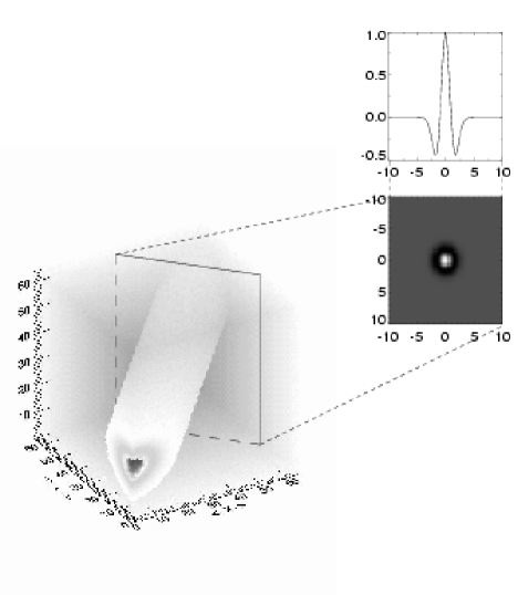
Figure 7 shows an example of beamlet function. It is constant along lines of direction ($\theta_{1}$, $\theta_{2}$), and a 2D wavelet function along plane orthogonal to this direction.

Figure 12: 3D beamlet transform flowgraph.

The 3D beamlet transform can be built using the ”Generalized projection-slice theorem” [39]. Let

• $f(\mathbf{x})$ an $n$ dimensional function,

• $\mathcal{R}ad_{m}f$ its m-dimensional partial radon transform along the first m cardinal directions, $m<n$, $\mathcal{R}ad_{m}f$ is a function of $(p,\mu_{m};x_{m+1},...,x_{n})$, $\boldsymbol{\mu}_{m}$ a unit directional vector in $\mathcal{R}ad_{m}$ (note that for a given projection angle, the $m$ dimensional partial radon transform of $f(\mathbf{x})$ has $(n-m)$ untransformated spatial dimension and a (n-m+1) dimensional projection profile),

• $\{\mathcal{F}f\}(\mathbf{k})$ its Fourier transform ($\mathbf{x}$ and $\mathbf{k}$ are conjugate variable pairs of $\mathcal{F}$),

The Fourier transform of the $m$ dimensional partial radon transform ${\cal R}_{m}f$ is related to the Fourier transform of $f$ $(\mathcal{F}f)$ by the following relation

$$\{\mathcal{F}_{n-m+1}\mathcal{R}ad_{m}f\}(k,k_{m+1},...,k_{n})=\{\mathcal{F}f\}(k\boldsymbol{\mu}_{m},k_{m+1},...,k_{n})$$ (12)

Let $c(i_{1},i_{2},i_{3})$ a cube of size $(N,N,N)$, the Beamlet algorithm consists in the following steps:

1. 3D-FFT. Compute $\hat{c}(k_{1},k_{2},k_{3})$, the three-dimensional FFT of the cube $c(i_{1},i_{2},i_{3})$.

2. Cartesian to Spherical Conversion. Using an interpolation scheme, substitute the sampled values of $\hat{c}$ obtained on the Cartesian coordinate system $(k_{1},k_{2},k_{3})$ with sampled values of on a spherical coordinate system $(\theta_{1},\theta_{2},\rho)$.

3. Extract planes. Extract the $3N^{2}$ planes (of size $N\times N$) passing through the origin (each line used in the 3D ridgelet transform defines set of orthogonal planes, we take the one which include the origin).

4. 2D-IFFT. Compute the two-dimensional inverse FFT on each plane.

5. 2D-WT. Compute the two-dimensional wavelet transform on each plane.

Figure 12 the 3D beamlet transform flowgraph. The 3D beamlet transform allows us to detect filament in a cube. The beamlet transform algorithm presented in this section differs from the one presented in [7], and relation between both algorithms is given in [6].

5 Experiments

5.1 Experiment 1

We have simulated three data set containing respectively a cluster, a plane and a line. On each data set, Poisson noise have been added with eight different background levels. Then we have applied the three transforms on the 24 simulated data set. The coefficients distribution related to each transformation is normalized using twenty realizations of a 3D flat distribution with a Poisson noise and which have the same number of counts as in the data.

Figure 13: Simulation of cubes containing a cluster (top), a plane (middle) and a line (bottom).

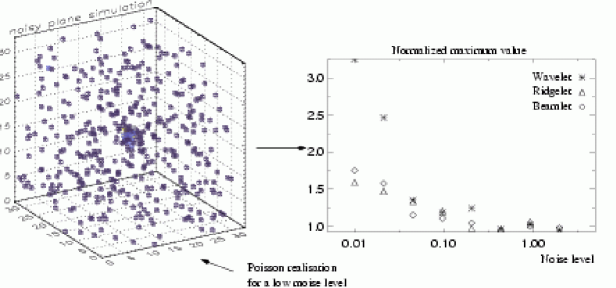
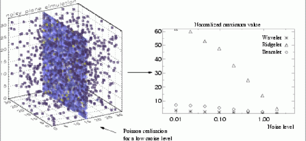
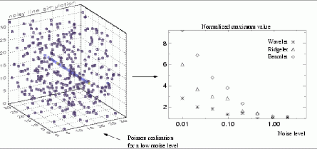
Figure 13 shows, from top to bottom, the maximum value of the normalized distribution versus the noise level for our three simulated data set. As expected, wavelets, ridgelets and beamlets are respectively the best for clusters, sheets and lines detection. It must also be underlined that a feature can be detected with a very high signal-to-noise ratio in a given basis, and and not detected in another basis. For example, the wall is detected at more than $60\sigma$ by the ridgelet transform, and less than $5\sigma$ by the wavelet transform. The line is detected almost at $10\sigma$ by the beamlet transform, and is under a $3\sigma$ detection level using wavelets. These results shows the importance of using several transforms for an optimal detection of all features contained in a data set.

5.2 Experiment 2

Figure 14: Simulated data sets. Top, the Voronoi vertices point pattern (left) and the galaxies of the GIF $\Lambda$-CDM N-body simulation (right). The bottom panels show one 10 $h^{-1}$ width slice of the each data set.

Figure 15: The two-point correlation function of the Voronoi vertices process and the GIF $\Lambda$-CDM N-body simulation. They are very similar in the range [0.02,2] $h^{-1}$ Mpc.

Figure 16: Skewness and kurtosis for the two simulated data set.

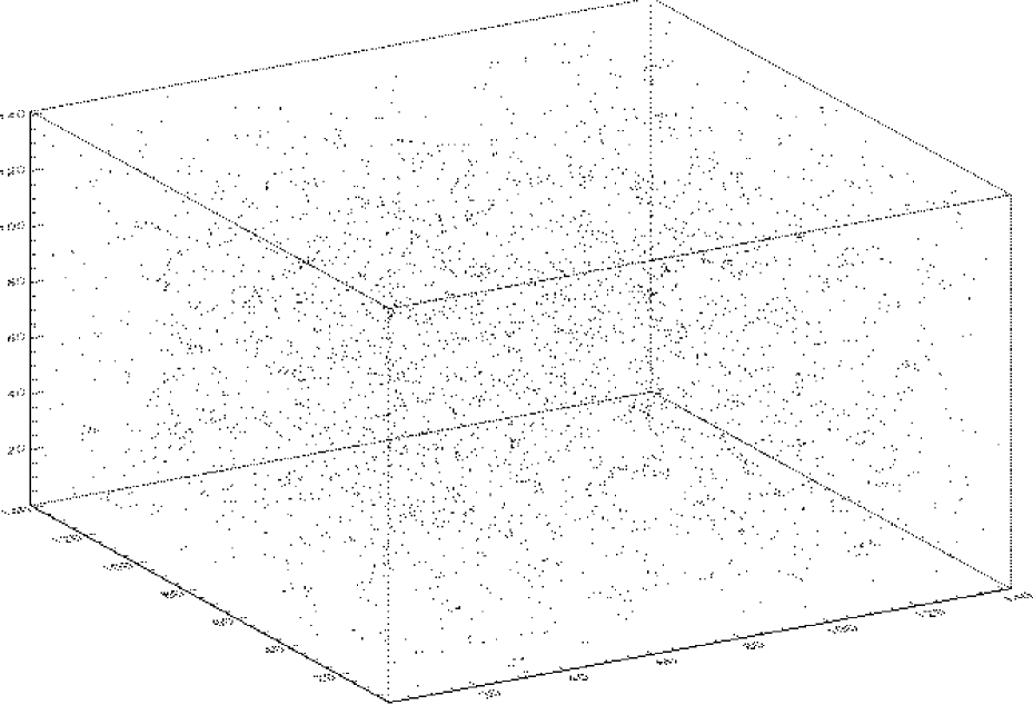
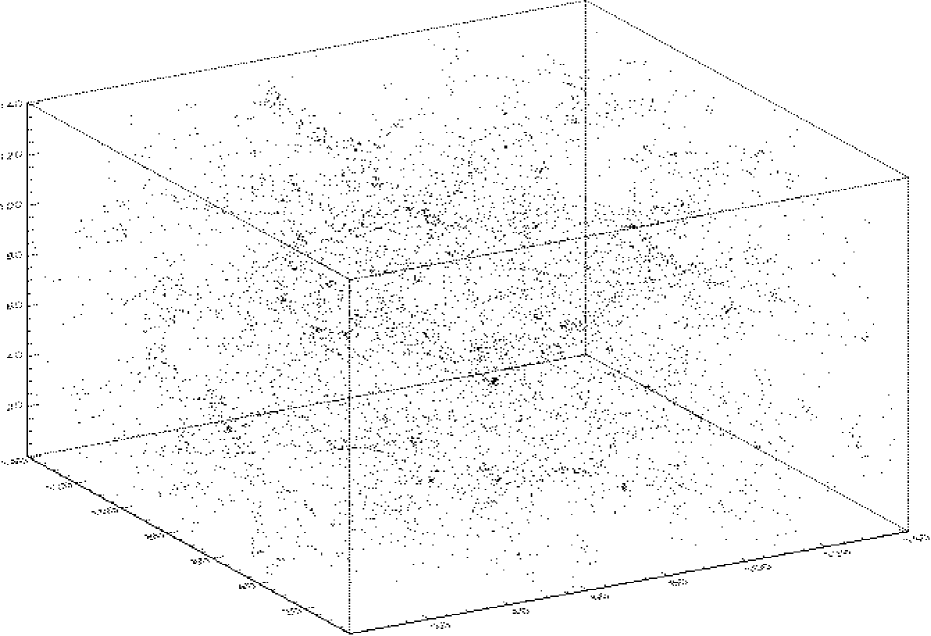
We use here two simulated data sets to illustrate the discriminative power of the multiscale methods. The first one is a simulation from stochastic geometry. It is based on a Voronoi model. The second one is a mock catalog of the galaxy distribution drawn from a $\Lambda$-CDM N-body cosmological model[12]. Both processes have very similar two-point correlation functions at small scales, although they look quite different and have been generated following completely different algorithms.

• the first comes from a Voronoi simulation: We locate a point in each of the vertices of a Voronoi tessellation of $1.500$ cells defined by $1500$ nuclei distributed following a binomial process. There are 10085 vertices lying within a box of 141.4 $h^{-1}$ Mpc side.

• the second point pattern represents the galaxy positions extracted from a cosmological $\Lambda$-CDM N-body simulation. The simulation has been carried out by the Virgo consortium and related groups (see http://www.mpa-garching.mpg.de/Virgo). The simulation is a low-density ($\Omega=0.3$) model with cosmological constant $\Lambda=0.7$. It is, therefore, the closer set to the real galaxy distribution[12]. There are 15445 galaxies within a box with side 141.3 $h^{-1}$ Mpc. Galaxies in this catalog have stellar masses exceeding $2\times 10^{10}$ $M_{\odot}$.

Figure 14 shows the two simulated data set, and Figure 15 shows the two-point correlation function curve for the two point processes. The two point fields are different, but as it can be seen in Fig. 15, both have very similar two-point correlation functions in a huge range of scales (2 decades).

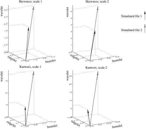
We have applied the three transforms to each data set, and we have calculated the skewness vector $S=(s^{j}_{w},s^{j}_{r},s^{j}_{b})$ and the kurtosis vector $K=(k^{j}_{w},k^{j}_{r},k^{j}_{b})$ at each scale $j$. $s^{j}_{w},s^{j}_{r},s^{j}_{b}$ are respectively the skewness at scale $j$ of the wavelet coefficients, the ridgelet coefficients and the beamlet coefficients. $k^{j}_{w},k^{j}_{r},k^{j}_{b}$ are respectively the kurtosis at scale $j$ of the wavelet coefficients, the ridgelet coefficients and the beamlet coefficients. Figure 16 shows the kurtosis and the skewness vectors of the two data set at the two first scales. On the contrary to the two-point correlation function, this analysis shows strong differences between the two data set, particularly on the wavelet axis, which indicates that the second data contains more, or with a higher density, clusters than the first one.

5.3 Experiment 3

In this experiment, we have used a $\Lambda$-CDM simulation based on a N-body and hydrodynamical code, called RAMSES [37]. The code is based on Adaptive Mesh Refinement (AMR) technique, with a tree-based data structure allowing recursive grid refinements on a cell-by-cell basis. The simulated data have been obtained using $256^{3}$ particles and $4.1\times 10^{7}$ cells in the AMR grid, reaching a formal resolution of $8192^{3}$. The box size was set to $100h^{-}1$ Mpc, with the following cosmological parameters:

$$\Omega_{m}=0.3 \Omega_{\lambda}=0.7 \Omega_{b}=0.039$$

$$h=0.7 \sigma_{8}=0.92$$ (13)

Figure 17: $\Lambda$-CDM simulation at different redshifts.

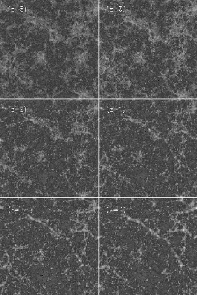
We used the results of this simulation at six different redshifts ($z=5,3,2,1,0.5,0$). Fig. 17 shows a projection of the simulated cubes along one axis. We have applied the 3D wavelet transform, the 3D beamlet transform and the 3D ridgelet transform on the six data set, and we calculate for each transform the standard deviation of the different scales. We will note $\sigma^{2}_{W,z,j},\sigma^{2}_{R,z,j},\sigma^{2}_{B,z,j}$ the variance of the scale $j$ relative to the transformation of the cube at redshift $z$ by respectively the wavelet, the ridgelet and the beamlet transform.

Figure 18: Top, Wavelet spectrum, middle, Beamlet spectrum, and bottom, ridgelet spectrum at different redshifts.

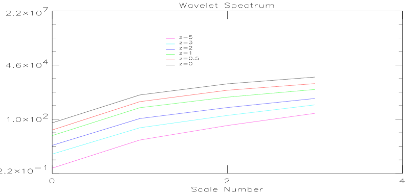
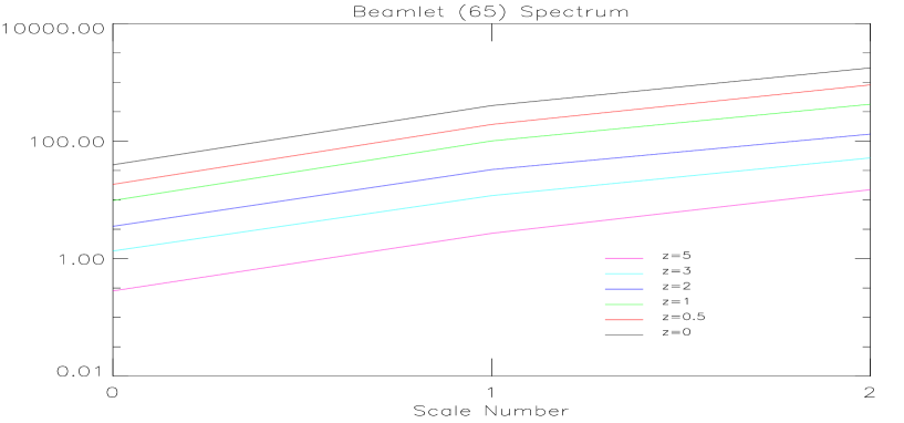
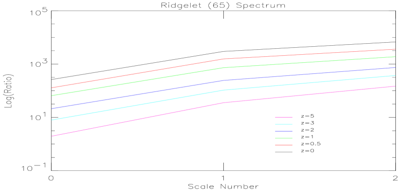
Figure 18 shows respectively from top to bottom the wavelet spectrum $P_{w}(z,j)=\sigma^{2}_{W,z,j}$, the beamlet spectrum $P_{b}(z,j)=\sigma^{2}_{B,z,j}$ and the ridgelet spectrum $P_{r}(z,j)=\sigma^{2}_{R,z,j}$. In order to see the evolution of matter distribution with the redshift and scale, we calculate the ratio $M_{bw}(j,z)=\frac{P_{b}(z,j)}{P_{w}(z,j)}$ and $M_{rw}(j,z)=\frac{P_{r}(z,j)}{P_{w}(z,j)}$.

Figure 19: $M_{1}(z,j)$ (top) and $M_{2}(z,j)$ (bottom) for the scale number $j$ equals to 1,2 and 3.

Figure 20: $M_{1}(z,j)$ (left) and $M_{2}(z,j)$ (right) at different redshifts.

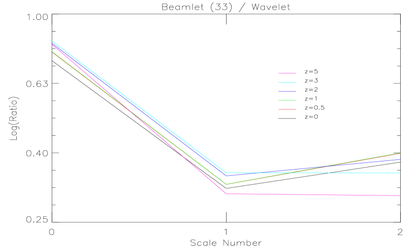
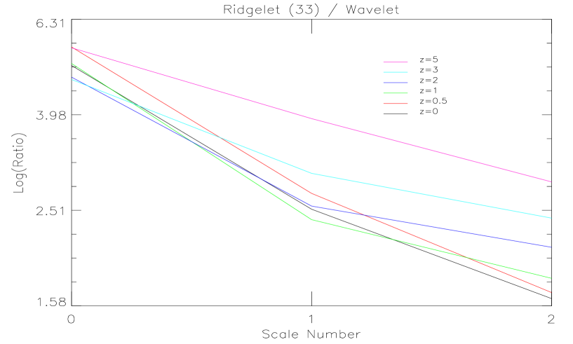
Figure 19 shows the $M_{1}$ and $M_{2}$ curves as a function of $z$ and Figure 20 shows the $M_{1}$ and $M_{2}$ curves as a function of the scale number $j$.

The $M_{1}$ curve does not show too much evolution, while the $M_{2}$ curve presents a significant slope. This shows that the beamlet transform is much more sensible to the formation of clusters than the ridgelet transform. This is not surprising since the beamlet function support is much smaller than the ridgelet function support. $M_{2}$ increases with $z$ showing clearly the cluster formation. This indicates that the combination of multiscale transformations allows us to get some information about the degree of clustering, filamentarity, and sheetedness.

6 Conclusion

We have introduced in this paper two new methods to analyze catalogs of galaxies. The first one consists in estimating the real underlying density though a wavelet denoising. Structures are first detected in the wavelet space, and an iterative reconstruction is performed. A smoothness constraint based on the $l_{1}$ norm of the wavelet coefficients is used, which reduce the amount of artifact in the reconstructed density, especially the ringing artifacts around strong features which are due to the wavelet function shape. We have shown that such an approach leads to much more reliable results than a Gaussian filtering when we want to derive a Genus curve from the catalog. This could also be true for other techniques which require to pre-process the data with a Gaussian filtering. The wavelet denoising preserves the resolution of the detected features whatever their sizes, and remove the noise in a non-linear way at all the scales.

The second approach does not require to detect anything. It is based on the analyzing of the distribution of coefficients obtained by several multiscale transforms. We have introduced two new multiscale decompositions, the 3D ridgelet transform and the 3D beamlet transform. We have described how to implement them using the FFT. Then we have shown that combining the information related to wavelet, ridgelet and beamlet coefficients leads to a new way to describe a data set. We have used in this paper the skewness and the kurtosis, but other recent statistic estimator such the Higher Criticism [5] could be used as well. Each multiscale transform is very sensible to one kind of feature, the wavelet to clusters, the beamlet to filaments, and the ridgelet to walls. A similar method has been proposed for analyzing CMB maps [29] where both the curvelet and the wavelet transform were used for the detection and the discrimination of non Gaussianities. This combined multiscale statistic is very powerful and we have shown that two data set that cannot be distinguished using a two point correlation function are clearly identified as different using our method. We believe that such an approach will permit to better constraint the cosmological models.

References

- [1] S. P. Bhavsar and R. J. Splinter. The superiority of the minimal spanning tree in percolation analyses of cosmological data sets. Monthly Notices of the Royal Astronomical Society, 282:1461–1466, October 1996.
- [2] E. J. Candès. Harmonic analysis of neural netwoks. Applied and Computational Harmonic Analysis, 6:197–218, 1999.
- [3] E.J. Candès and D. Donoho. Ridgelets: the key to high dimensional intermittency? Philosophical Transactions of the Royal Society of London A, 357:2495–2509, 1999.
- [4] D. Donoho and X. Huo. Lecture Notes in Computational Science and Engineering, chapter Beamlets and Multiscale Image Analysis. Springer, 2001.
- [5] D. Donoho and J. Jin. Higher criticism for detecting sparse heterogeneous mixtures. Technical Report , Statistics Department, Stanford University, 2002.
- [6] D.L. Donoho and O. Levi. Fast X-Ray and Beamlet Transforms for Three-Dimensional Data. In D. Rockmore and D. Healy, editors, Modern Signal Processing, 2002.
- [7] D.L. Donoho, O. Levi, J.-L. Starck, and V.J. Martínez. Multiscale geometric analysis for 3-d catalogues. In J.-L. Starck and F. Murtagh, editors, SPIE conference on Astronomical Telescopes and Instrumentation: Astronomical Data Analysis II, Waikoloa, Hawaii, 22-28 August, volume 4847. SPIE, 2002.
- [8] A. G. Doroshkevich, D. L. Tucker, R. Fong, V. Turchaninov, and H. Lin. Large-scale galaxy distribution in the Las Campanas Redshift Survey. Monthly Notices of the Royal Astronomical Society, 322:369–388, April 2001.
- [9] E. Escalera, E. Slezak, and A. Mazure. New evidence for subclustering in the Coma cluster using the wavelet analysis. Astronomy and Astrophysics, 264:379–384, October 1992.
- [10] J. R. Gott, M. Dickinson, and A. L. Melott. The sponge-like topology of large-scale structure in the universe. Astrophysical Journal, 306:341–357, July 1986.
- [11] C. Hikage, Y. Suto, I. Kayo, A. Taruya, T. Matsubara, M. S. Vogeley, F. Hoyle, J. R. I. Gott, and J. Brinkmann. Three-Dimensional Genus Statistics of Galaxies in the SDSS Early Data Release. Publications of the Astronomical Society of Japon, 54:707–717, October 2002.
- [12] G. Kauffmann, J. M. Colberg, A. Diaferio, and S. D. M. White. Clustering of galaxies in a hierarchical universe - I. Methods and results at z=0. Monthly Notices of the Royal Astronomical Society, 303:188–206, 1999.
- [13] M. Kerscher. Statistical analysis of large-scale structure in the Universe. In K. Mecke and D. Stoyan, editors, Statistical Physics and Spatial Satistics: The Art of Analyzing and Modeling Spatial Structures and Pattern Formation. Lecture Notes in Physics 554, 2000.
- [14] M. Kerscher, M.J. Pons-Bordería, J. Schmalzing, R. Trasarti-Battistoni, T. Buchert, V.J. Martínez, and R. Valdarnini. A global descriptor of spatial pattern interaction in the galaxy distribution. Astrophysical Journal, 513:543–548, 1999.
- [15] L. G. Krzewina and W. C. Saslaw. Minimal spanning tree statistics for the analysis of large-scale structure. Monthly Notices of the Royal Astronomical Society, 278:869–876, February 1996.
- [16] T. Kurokawa, M. Morikawa, and H. Mouri. Scaling analysis of galaxy distribution in the Las Campanas Redshift Survey data. Astronomy and Astrophysics, 370:358–364, May 2001.
- [17] M.N.M. Van Lieshout and A.J. Baddeley. A non parametric measure of spatial interaction in point patterns. Statistica Neerlandica, 50:344–361, 1996.
- [18] V. J. Martínez, B. J. T. Jones, R. Domínguez-Tenreiro, and R. van de Weygaert. Clustering paradigms and multifractal measures. Astrophysical Journal, 357:50–61, 1990.
- [19] V. J. Martínez, S. Paredes, and E. Saar. Wavelet analysis of the multifractal character of the galaxy distribution. Monthly Notices of the Royal Astronomical Society, 260:365–375, 1993.
- [20] V. J. Martínez and E. Saar. Statistics of the Galaxy Distribution. Chapman and Hall/CRC press, Boca Raton, 2002.
- [21] S. Maurogordato and M. Lachieze-Rey. Void probabilities in the galaxy distribution — scaling and luminosity segregation. Astrophysical Journal, 320:13–25, 1987.
- [22] K. R. Mecke, T. Buchert, and H. Wagner. Robust morphological measures for large-scale structure in the Universe. Astronomy and Astrophysics, 288:697–704, August 1994.
- [23] A. Pagliaro, V. Antonuccio-Delogu, U. Becciani, and M. Gambera. Substructure recovery by three-dimensional discrete wavelet transforms. Monthly Notices of the Royal Astronomical Society, 310:835–841, December 1999.
- [24] P.J.E. Peebles. The Large-Scale Structure of the Universe. Princeton University Press, 1980.
- [25] P.J.E. Peebles. The galaxy and mass N-point correlation functions: a blast from the past. In V.J. Martínez, V. Trimble, and M.J. Pons-Bordería, editors, Historical Development of Modern Cosmology, Astronomical Society of the Pacific, 2001. ASP Conference Series.
- [26] V. Sahni, B. S. Sathyaprakash, and S. F. Shandarin. Shapefinders: A New Shape Diagnostic for Large-Scale Structure. Astrophysical Journal Letters, 495:L5+, March 1998.
- [27] J. V. Sheth, V. Sahni, S. F. Shandarin, and B. S. Sathyaprakash. Measuring the geometry and topology of large-scale structure using SURFGEN: methodology and preliminary results. Monthly Notices of the Royal Astronomical Society, 343:22–46, July 2003.
- [28] E. Slezak, V. de Lapparent, and A. Bijaoui. Objective detection of voids and high density structures in the first CfA redshift survey slice. Astrophysical Journal, 409:517–529, 1993.
- [29] J.-L. Starck, N. Aghanim, and O. Forni. Detecting cosmological non-gaussian signatures by multi-scale methods. Astronomy and Astrophysics, 416:9–17, 2004.
- [30] J.-L. Starck, A. Bijaoui, and F. Murtagh. Multiresolution support applied to image filtering and deconvolution. CVGIP: Graphical Models and Image Processing, 57:420–431, 1995.
- [31] J.-L. Starck, E. Candès, and D.L. Donoho. The curvelet transform for image denoising. IEEE Transactions on Image Processing, 11(6):131–141, 2002.
- [32] J.-L. Starck and F. Murtagh. Astronomical Image and Data Analysis. Springer-Verlag, 2002.
- [33] J.-L. Starck, F. Murtagh, and A. Bijaoui. Image Processing and Data Analysis: The Multiscale Approach. Cambridge University Press, 1998.
- [34] J.-L. Starck and M. Pierre. Structure detection in low intensity X-ray images. Astronomy and Astrophysics, Supplement Series, 128, 1998.
- [35] S. Szapudi and A. S. Szalay. A new class of estimators for the N-point correlations. Astrophysical Journal Letters, 494:L41, February 1998.
- [36] M. Tegmark, M. R. Blanton, M. A. Strauss, F. Hoyle, D. Schlegel, R. Scoccimarro, M. S. Vogeley, D. H. Weinberg, I. Zehavi, A. Berlind, T. Budavari, A. Connolly, D. J. Eisenstein, D. Finkbeiner, J. A. Frieman, J. E. Gunn, A. J. S. Hamilton, L. Hui, B. Jain, D. Johnston, S. Kent, H. Lin, R. Nakajima, R. C. Nichol, J. P. Ostriker, A. Pope, R. Scranton, U. Seljak, R. K. Sheth, A. Stebbins, A. S. Szalay, I. Szapudi, L. Verde, Y. Xu, J. Annis, N. A. Bahcall, J. Brinkmann, S. Burles, F. J. Castander, I. Csabai, J. Loveday, M. Doi, M. Fukugita, J. R. I. Gott, G. Hennessy, D. W. Hogg, Ž. Ivezić, G. R. Knapp, D. Q. Lamb, B. C. Lee, R. H. Lupton, T. A. McKay, P. Kunszt, J. A. Munn, L. O’Connell, J. Peoples, J. R. Pier, M. Richmond, C. Rockosi, D. P. Schneider, C. Stoughton, D. L. Tucker, D. E. Vanden Berk, B. Yanny, and D. G. York. The Three-Dimensional Power Spectrum of Galaxies from the Sloan Digital Sky Survey. Astrophysical Journal, 606:702–740, May 2004.
- [37] R. Teyssier. Cosmological hydrodynamics with adaptive mesh refinement. A new high resolution code called RAMSES. Astronomy and Astrophysics, 385:337–364, April 2002.
- [38] Isao Yamada. The hybrid steepest descent method for the variational inequality problem over the intersection of fixed point sets of nonexpansive mappings. In D. Butnariu, Y. Censor, and S. Reich, editors, Inherently Parallel Algorithms in Feasibility and Optimization and Their Applications. Elsevier, 2001.
- [39] Paul C. Lauterbur Zhi-Oei Liang. Principle of Magnetic Resonance Imaging. IEEE Press, 2000.