Long-Term Behavior of X-ray Pulsars in the Small Magellanic Cloud

Abstract

Results of a 4 year X-ray monitoring campaign of the Small Magellanic Cloud using the Rossi X-ray Timing Explorer (RXTE) are presented. This large dataset makes possible detailed investigation of a significant sample of SMC X-ray binaries. 8 new X-ray pulsars were discovered and a total of 20 different systems were detected. Spectral and timing parameters were obtained for 18. In the case of 10 pulsars, repeated outbursts were observed, allowing determination of candidate orbital periods for these systems. We also discuss the spatial, and pulse-period distributions of the SMC pulsars.

1 The Survey

A program of regular observations of the Small Magellanic Cloud (SMC) using the Rossi X-ray Timing Explorer (RXTE) has been underway since 1997, in conjunction with optical imaging and spectroscopic follow-up observations. New SMC pulsars discovered by RXTE have been reported in a number of publications, and this work is intended to present the wealth of long-term data now accumulated for these sources. This paper reports the results of 4 years (November 1997 - February 2002) of weekly monitoring and presents the long-term behavior of most of the known X-ray pulsar systems. During this time, 16 X-ray pulsars were discovered by RXTE, at the same time many discoveries were made by ASCA and BeppoSAX, bringing the number of known X-ray pulsars in the SMC to 30.

Long term pulsed-flux lightcurves of all pulsars observed during the project are presented. Twenty pulsars were positively detected in the data presented in this paper, and upper limits were placed on 6 other known pulsars that were not detected during this time. In the case of 15 systems, multiple X-ray outbursts were observed, raising the possibility of determining orbital periods. Interpretation of the findings, in terms of the overall SMC population is discussed.

RXTE is particularly well suited to monitoring pulsars in the SMC. The Proportional Counter Array (PCA) is able to cover a significant fraction of the SMC at sufficient sensitivity to detect active pulsars with luminosities in the typical range 10³⁶-10³⁸ ${\rm\thinspace erg}{\rm\thinspace s}^{-1}$. The spectral response is also favorable as the construction of the PCA provides its optimum sensitivity across the peak of the typical pulsar spectrum. The PCA’s full-width zero intensity (FWZI) field of view is 2^∘ and the instrument is non-imaging. However, the PCA can be scanned across a target region and the location of a bright source determined to an accuracy of 1-2$\arcmin$ by fitting the collimator response to the observed count-rate.

The low extinction and unobstructed line of sight to the SMC enable accurate measurements of X-ray luminosity and useful observations of the optical counterparts with 1-2m telescopes (see for example Edge & Coe, 2003). From the X-ray viewpoint, since the distance to the SMC is significantly greater than its ’depth’ all of the objects in the SMC can be considered to lie at an equal distance for the purposes of luminosity calculations.

1.1 Observing Strategy

The RXTE Proportional Counter Array (PCA) (Jahoda et al, 1996) was used to make regular observations of the SMC to look for new X-ray pulsars and monitor the outbursts of known systems. The instrument consists of 5 co-aligned Proportional Counter Units (PCU), each has a xenon filled detector volume with 3 layers of anode-grids for photon detection plus a lower xenon veto layer for background rejection. Propane-filled veto detectors are positioned above the PCA to attenuate particle background and non-source direction X-rays. Operated in Good Xenon mode, individual photon arrival times are recovered to 1$\mu$s accuracy, and pulse-heights processed into 256 channels between 2-100 keV. According to the ABC of XTE the top layer of the PCA is the most sensitive, with the majority of source events occurring there, while the background rate is similar in all 3 layers. We verified that the detection significance for pulsars is slightly better using layer 1 only versus layers 1 and 2, when extracting lightcurves in the 2-10 keV band.

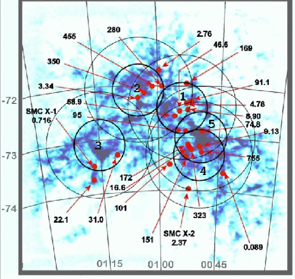
Figure 1: RXTE observations in the SMC. Circles show the PCA field of view in the most-used monitoring positions. The pointing centers are listed in Table 1. The background image is an HI radio map by Stanimirovic et al (1999). The positions of known pulsars are indicated by their pulse periods.

The program began after a new X-ray transient was detected during a PCA slew in the vicinity of SMC X-3 (Marshall, Lochner & Takeshima, 1997). A PCA observation was conducted on 1997 November 29 in response to this detection, revealing not SMC X-3 but three previously unknown pulsars with pulse periods of 91.s, 74s and 46.6s (Corbet et al, 1998). Continued observations throughout December and January detected 2 more pulsars with periods of 169s (Lochner et al, 1998a) and 58.9s (Marshall et al, 1998). At times observations were being made at a rate of 1 per day, giving excellent temporal coverage of the outbursts of these pulsars. Following these observations, a program of regular monitoring was established (see Table 1), with pointed PCA observations of several ksec duration made on a weekly basis. Pointing positions were carefully chosen to give good coverage of the main body of the SMC, as shown in Figure 1. The “wing” was not regularly observed due to the presence of the luminous supergiant High-Mass X-ray Binary (HMXB) SMC X-1. This source was deliberately excluded from the PCA survey because its persistent emission, very strong pulsations, and timing noise mask the presence of other weaker pulsars when it is in the field of view. Observations were made in 3 phases during which slightly different observing strategies have been employed, as described below.

Phase 1. This comprises the series of observations conducted and described by Lochner et al (1999). The observations were made primarily in two positions designated 1a and 1c. Position 1a was centered on the location of SMC X-3, because the initial source detected was at first thought to be SMC X-3. Position 1b was the position of a single PCA pointing aimed at the location of one of the new pulsars. Position 1c lies close by and was used throughout 1998 to monitor the activity of the 4 newly discovered pulsars mentioned above.

Phase 2. During this period we continued to monitor the known pulsars and at the same time search for new sources. Position 1 largely overlaps with the fields of view of the earlier observations. Position 3 was chosen to cover the eastern wing of the SMC which contains SMC X-1. Positions 2 and 4 were chosen to cover the rest of the SMC.

Phase 3. After 2 years of monitoring position 1, we broadened the search by shifting south to position 5, also in the main body of the SMC. The supplementary positions 2, 3 and 4 were not observed, as previous observations of these positions caused gaps in coverage of the main position. Position 5 was observed each week for 2.1 years.

1.2 Data Reduction Pipeline

Data reduction was performed in two stages, “real-time monitoring” and “survey”: Immediately after each routine PCA observation, quick-look data were searched for new pulsars. Initially a lightcurve was generated at 3-10 keV and 0.1 second time resolution. No filtering criteria or background subtraction were applied at this stage. The power spectrum was inspected visually and with a peak search algorithm. This preliminary data analysis was usually performed within a day or so of the observation taking place, to identify new pulsars and schedule rapid TOO follow-up observations. The long-term survey made use of the production data, and more detailed analysis methods. All data reduction was done with Ftools. Standard filtering criteria were applied to exclude data collected during: periods of high background; times when the source was attenuated by Earth’s atmosphere; during slews on/off source; and times immediately after SAA passage. On 2000 May 20 the upper propane veto-layer of PCU 0 was lost, after that date PCU 0 data were excluded. Filtering by detector/layer was performed with bit-masks generated by sefilter.

Background count-rates were generated using pcabackest and the L7 models for faint sources. Lightcurves and spectra were extracted from the generated background using saextrct with the same filtering criteria and detector/layer combinations as were applied to the science data.

1.2.1 Lightcurve Extraction

Science lightcurves were extracted using seextrct at 0.01 second time binning for the 3-10 keV Good Xenon data from the top anode layer of each active PCU. This configuration maximizes signal-to-noise for pulsars. Background lightcurves were extracted with 16s binning (the minimum available) and subtracted from the science lightcurve, without modifying the errors on the science count-rates.

The lightcurve was then normalized to ${\rm\thinspace counts}{\rm\thinspace PCU}^{-1}{\rm\thinspace s}^{-1}\,$, by dividing each flux value by the number of PCUs active at that time. Lightcurve bin-times were corrected for the motion of the satellite and Earth’s orbit using faxbary to give the arrival times at the solar system barycenter.

1.2.2 Correcting for Collimator Response

For every pulsar with a well known position, the detector sensitivity ($R$) was calculated at each pointing position. The collimator for each PCU are constructed from corrugated sheets with hexagonal cells. The hexagonal cells have small offsets in pointing direction and the angular responses for each PCU are different. For the purposes of examining long term light curves we adopt a simplified model for the collimators of a circular field of view with a simple triangular collimator response of full-width half maximum (FWHM) = 1°, full-width zero intensity (FWZI) = 2°. This simplified model differs from the true collimator response in being somewhat sharper peaked, lacking extended wings at larger angles (where we do not have significant pulsar detections) and lacking the hexagonal symmetry which is also most pronounced at larger offset angles. The use of this simplified model speeds data analysis and is not a significant factor in, for example, searching for periodic behavior. With our simplified collimator model, for a particular pulsar at known distance from the pointing center, $R$ equals 1.0 minus the net pointing offset in degrees. Values of R for each pulsar in each of the monitoring positions are listed in Table 7. This table should be consulted when examining the long-term pulsar lightcurves in Section 3. It is apparent that the scatter in flux measurements is correlated with $R$. Blank entries in Table 7 indicate that the pulsar was not in the field of view. In practice, observations at marginal sensitivity were also excluded. A value of $R<0.1$ was regarded as marginal and a lightcurve not extracted for observations of that particular pulsar/pointing position combination. For spectral analysis in this paper we utilize the full detailed model of collimator response for those sources with accurate positions.

1.3 Timing Analysis

The methods used to measure pulse periods, pulse amplitudes, calculate significance levels and reject false detections are outlined here.

A Lomb-Scargle periodogram (Scargle, 1982) was calculated for each observation, scanning the range 0.02-1000 s at a resolution of $1\times 10^{-5}$ Hz. Also generated by the pipeline were statistical parameters used in assigning significance levels and converting between spectral power and pulsed flux.

The special properties of the Lomb-Scargle periodogram were exploited to scan every observation around the period of each known pulsar. We first determined if there was $significant$ power at a given (known pulsar) frequency and then determined its period and amplitude, if however there was non-zero power at a low significance level, an upper limit was placed on the pulse-amplitude of the (presumably inactive) pulsar.

For each known pulsar, (i.e those detected at a high level of confidence in one or more observations, or from the literature) an appropriate period search-range was determined from inspection of occurrences detected at $\geq$ 90% significance in a blind search. For “literature” pulsars a $\pm$5% frequency band centered on the known period was used. The Lomb-Scargle periodogram of each observation was then scanned in this period range, the maximum power identified and its significance estimated, considering only the independent frequencies in the allowed period range. This is the prior knowledge significance.

Given that 30 SMC pulsars are known with periods less than 1000 s, allowing for up to 3 harmonics gives a possible 93 genuine signal frequencies. Once period variability and timing resolution are included, the possibility of contamination requires the adoption of an algorithm to reject false detections of pulsars that lie close to the harmonic frequencies of others.

If the maximum power recorded was not a peak inside the selected range, i.e. it lay at edge of the frequency range, then it was assumed to be leakage of power from a nearby and unrelated frequency. Whenever this situation occurred, the detection significance was set to zero since the probability that the power was due to the pulsar being searched for is negligible. For positive detections the pulse period and its uncertainty were also recorded. The uncertainty on the period was calculated using the formulation of Kovacs (1980) which accounts for the strength of the detected signal.

For each pulsar we only considered observations of duration greater than 4 pulsation cycles otherwise there are unacceptably large errors on the pulse period and poor confidence in their identification.

For each positive detection, the measured power $P_{LS}$ was converted into a pulse amplitude using Equation 1: where the lightcurve has $N_{P}$ points and variance $\sigma^{2}$, the peak-to-valley amplitude (twice the sinusoidal amplitude) $A^{\ast}$ of a signal detected in the Lomb-Scargle periodogram is:

$$A^{\ast}=4\sqrt{\frac{P_{LS}\sigma^{2}}{N_{P}}}$$ (1)

The significance of peaks in the Lomb-Scargle periodogram is described by a simple exponential function, related to the number of independent frequencies in the range being searched in the case of periodic signals superimposed on white noise with a Gaussian distribution. The significance calculations in this work follow the prescription of Press et al (1993).

The precise nature of the data sampling is relevant in timing analysis. Data gaps are unavoidable and applying barycenter correction to the lightcurve bin times causes a small departure from regular sampling. Random sampling is $recommended$ by Scargle (1982) in order to maximize the anti-aliasing properties of the Lomb-Scargle periodogram, but clumpy or gappy data are not handled so efficiently and, in cases involving one or two large gaps in otherwise regular data, aliasing is similar to a Discrete Fourier Transform. We used the fast coding of Press & Rybicki (1989).

1.4 Flux Measurements

Throughout this paper we use units of ${\rm\thinspace counts}{\rm\thinspace PCU}^{-1}{\rm\thinspace s}^{-1}\,$, these can be approximately compared to the flux in ${\rm\thinspace erg}{\rm\thinspace cm}^{-2}{\rm\thinspace s}^{-1}\,$if assumptions are made regarding the X-ray photon spectral index ($\alpha$) and line-of-sight absorption column-density ($N_{H}$). Taking reasonable values for X-ray pulsars to be $\alpha=1,N_{H}=1\times 10^{22}cm^{-2}$ gives an approximate conversion factor of 1${\rm\thinspace counts}{\rm\thinspace PCU}^{-1}{\rm\thinspace s}^{-1}\,$= 1.2$\times 10^{-11}$${\rm\thinspace erg}{\rm\thinspace cm}^{-2}{\rm\thinspace s}^{-1}\,$. At the SMC (65 kpc), this corresponds to a luminosity of $L_{X}=5.7\times 10^{36}\ erg\ s^{-1}$. Pulse amplitude is simply related to the pulsed flux (pulsed component summed over a full cycle) by a factor of 2. The total flux can only be determined if the pulse fraction (ratio of pulsed to unpulsed component) is known. We choose to discuss the pulse amplitude as this is the most directly measurable quantity and enables robust measurements to be made even when multiple pulsars are present in a single observation.

1.5 Orbital Period Estimation

One of our primary goals was to measure orbital periods for the X-ray sources. This was done by analyzing the long-term pulsed-flux lightcurves produced by our pipeline. In prototypical Be-X systems, X-ray outbursts occur in periodic sequences. Many of our lightcurves presented in Section 3 show such features, for example XTE J0055-724 (Figure 14). In these cases we employed Phase Dispersion Minimization (PDM, Stellingwerf, 1978), which is the most appropriate technique to search for highly irregular modulations which are also poorly sampled.

Systems such as AX J0049.4-7323 (Figure 39) presented two outbursts which, although insufficient to formally claim a “period”, have nonetheless proved to be highly reliable indicators of the orbital period. If two outbursts are seen from the same Be system within a recurrence time of several weeks, we know from the underlying physics that these are highly likely to be separated by one orbital period. Measurement of such “recurrence times” was done by folding the dates of significant detections on a range of trial periods, and selecting the period that produced the minimum scatter in phase. This is similar to taking the mean separation of outbursts, but includes multiple data-points for each outburst, and accounts for the fact that we do not know the date of outburst-maximum very well, due to sparse sampling. The uncertainty is calculated by multiplying the minimum standard deviation in phase by the best period. We term this method “simple timing analysis” (STA). Given the small number of points available (typically 4-20), STA results are a “best estimate” only.

In other cases (e.g. AX J 0051.6-7311, see Figure 30) the long-term lightcurve contains many detections of the pulsar on dates that do not form an obvious periodic sequence. The explanations include X-ray emission that is genuinely aperiodic, as well as missed outbursts which could hide an underlying periodic pattern. These cases were analyzed with both PDM and STA and the most likely periods or recurrence times reported, in order to provide a guide for other observers.

Finally a few systems (e.g. SMC X-2) have undergone a single giant outburst during our monitoring project. In these cases no orbital periods could be measured, instead pulse-period variations were used to constrain the contributions from orbital motion (Doppler shifts) and accretion torques.

2 Results I: Pulsar Monitor Charts

After reduction, the data were analyzed in 2 separate ways to search for variable sources, the first of these is the blind search.

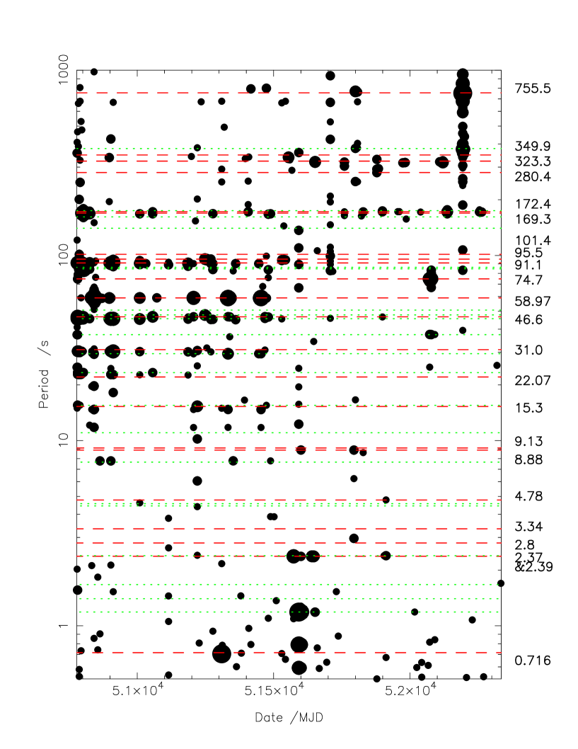
Figure 2: Activity chart for pulsars detected in all of the regular pointing positions between 1997 November 27 and 2002 February 28. Relative pulsation strength is indicated by marker size. No selection criteria have been applied other than a significance threshold. All power at greater than 90% blind search significance is plotted.

Having generated the Lomb-Scargle periodogram for every observation, the resulting database of periodograms was searched for significant peaks. The significance level for each observation was estimated individually. This stage was executed as a “blind search”, the threshold adopted was 90% significance considering all frequencies in the (period) range 0.5 -1000 seconds. We used a simple boxcar peak-search algorithm which identified a peak as any frequency having a greater power than its nearest neighbors, subject to that power being above the 90% significance level. Figure 2 displays the combined results of this analysis in the form of a “pulsar activity monitor”, showing the activity of bright pulsars in all the monitoring positions. The size of the graph markers indicates spectral power on a logarithmic scale, horizontal dashed lines (red) indicate pulse periods of the majority of known pulsars in the SMC, these periods are given on the right of the plot. In addition to detecting pulse periods, this procedure also picks up harmonics and, in principle at least, low frequency quasi-periodic oscillations. In particular it has been observed in the course of this work that at times the $P_{pulse}/2$ harmonic can dominate the power spectrum. Therefore all significant power is included on the plots. The expected $P_{pulse}/2$ harmonics of known pulsars are indicated by dotted (green) lines. As the various pointing positions cover partially overlapping fields of view, different pulsars are visible in subsets of the data. Positions 1 and 5 comprise the bulk of the data.

Figure 2 shows pulsars ranging in period from 0.7s (SMC X-1) to 755s (AX J0049.4-7323). It is immediately apparent that two sources were particularly active throughout the survey. The 172.4s and 323s pulsars appear to have undergone respectively 5 and 7 outbursts over a period of about 700 days. If these outbursts are normal Be/X-ray binary outbursts then the results are suggestive of orbital periods of (very) approximately 700/5=140d and 700/7=100d. The line labeled “2.37 & 2.39” is also of particular interest as the points lying along it actually belong to two different pulsars. The group of points at about MJD 51600 is due to an outburst from SMC X-2, Below these points, 2^nd, 3^rd and 4^th harmonics are visible. There then follows a short ($\sim$ 2 week) break in observing coverage after which the pulsations were again detected but visibly weaker and with the relative strength of the harmonics altered. Just after MJD 51900 a third group of points appear on the “2.37 & 2.39” line, these are the first harmonic of XTE J0052-723 which was first discovered in these observations, the fundamental is seen just once on this plot.

No sub-second pulsars were detected, only 3 observations containing significant peaks at P$<$1s were ever seen:

(1) A single detection of the (P/2) harmonic of SMC X-1; and 2 harmonics of SMC X-2 (P/5 and P/6).

(2) On MJD 51381, period 0.0329429(5)s, amplitude 0.73 ${\rm\thinspace counts}{\rm\thinspace PCU}^{-1}{\rm\thinspace s}^{-1}\,$, significance above 99% in one 1050s observation. However two other observations on the same day, of comparable length made  1 hr before and  1 hr after failed to show any evidence for this period.

(3) On MJD 51432, period 0.0747731(3)s, amplitude 0.31 ${\rm\thinspace counts}{\rm\thinspace PCU}^{-1}{\rm\thinspace s}^{-1}\,$, significance 97%. It is expected that a small number of false detections will occur given the large number of observations analyzed and this low significance detection may thus not be real.

3 Results II: Long Term Pulsar Lightcurves

Long term behavior of all known pulsars in the SMC was investigated using the database of Lomb-Scargle periodograms generated from the RXTE monitoring observations.

In the following section the pulsars are ordered by pulse period. Trends in physical characteristics are likely to follow the pulse period, so it is appropriate to list the systems in a natural sequence that facilitates comparison.

The most important results are shown in a series of 3-panel plots for each source, laid out as follows:

Top panel. Pulsed flux lightcurve, filled symbols indicate positive detections, open symbols are upper limits.
Middle panel. Pulse period with uncertainty.
Lower Panel. Statistical significance of each pulsed flux measurement. Two significance estimators are plotted: Blind search (squares), and prior knowledge of period (circles). The criterion for a positive detection was 99% prior knowledge significance. Blind search significance values are shown in order to convey those detections of outstanding magnitude.

3.1 SMC X-2 (2.37s)

SMC X-2 was discovered by SAS-3 in 1978 (Clarke et al, 1978) and although outbursts were also observed by HEAO 1 and ROSAT, pulsations had not been detected until the RXTE monitoring data presented here.

A single outburst was detected from SMC X-2, lasting from 2000 January 24 to April 23. During this outburst, the luminosity (2-25 keV) reached a peak of 4.7 $\times 10^{38}\mbox{${\rm\thinspace erg}{\rm\thinspace s}^{-1}$}$, and was detected down to a level of 5.7$\times 10^{37}\mbox{${\rm\thinspace erg}{\rm\thinspace s}^{-1}$}$ before disappearing from view sometime before May 5. The detection of SMC X-2 with the RXTE All-Sky Monitor (ASM) followed by discovery of 2.37 second pulsations co-incident with the known position of SMC X-2 from PCA scans and targeted observations was presented by Corbet et al (2001), along with contemporaneous optical observations confirming the counterpart originally proposed by Murdin et al (1993). An ASCA observation on April 24 by Yokogawa et al (2001) confirmed the 2.37 s pulsar to be exactly coincident with the position of SMC X-2 determined by SAS-3 and ROSAT .

From the SMC monitoring data, pulsations with a period of 2.37s were detected with the PCA during 13 observations between MJD 51567 and MJD 51657. Of these, 9 were pointings at the regular monitoring position (position 5, see Table 1), plus 2 targeted pointings centered on SMC X-2, and 2 sets of scans across the source region. All of these observations are included in the long-term lightcurve (Figure 3).

The duration of the outburst was constrained by non-detections before and after the dates given in Table 2, on MJD 51560 and 51666-7 and 51670. The upper limits for the end of the outburst are more stringent as these observations were pointed directly at the position of SMC X-2.

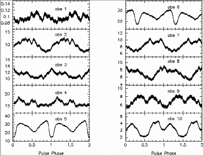
Figure 4: Pulse profiles of SMC X-2 during the January - April 2000 outburst. Flux in units of ${\rm\thinspace counts}{\rm\thinspace PCU}^{-1}{\rm\thinspace s}^{-1}\,$for the 2 - 10 keV band, arbitrary phase. Collimator correction and background subtraction have been applied.

Due to changes is the power spectrum of SMC X-2 during the outburst, pulse periods were refined by PDM (Stellingwerf, 1978). The refined periods are given in Table 2. The pulse profiles (Figure 4) obtained during the outburst show an interesting trend with luminosity. During the low luminosity observations at the beginning and end of the outburst, the pulse profile was a weakly double peaked shape, with roughly equal peaks separated by half a cycle: typical of that seen in many X-ray pulsars. At high luminosity the shape changed, with peak flux occurring either side of a narrow minimum, the separation between the first and second peak now 0.7 in phase. This change was seen in the power spectra as a reversal in the normal ratio of the fundamental and 1st harmonic: evident from the pulsar monitor (Figure 2) around MJD 51600. For this reason the pulse amplitudes plotted in Figure 3 are derived either from the fundamental or harmonic depending on which was the stronger.

The X-ray spectrum of SMC X-2 was extracted for 3 observations, the two targeted pointings (Corbet et al, 2001) and observation 5 when the highest flux was observed. Assuming the spectral parameters in Table 3 to be reasonably representative of SMC X-2 during the whole outburst ($N_{H}=2\times 10^{22}$ cm^-2, $\alpha=1$) the fluxes reported in Table 2 may be converted to $L_{X}$ by $1\hbox{${\rm\thinspace counts}{\rm\thinspace PCU}^{-1}{\rm\thinspace s}^{-1}\,$}=1.72\times 10^{37}\mbox{${\rm\thinspace erg}{\rm\thinspace s}^{-1}$}$ assuming a 65 kpc distance to the SMC.

3.1.1 In-outburst Timing Behavior

Period variations evident in Figure 3 are suggestive of spin-up or orbital modulation, these measurements were investigated and refined by Phase Dispersion Minimization (PDM). The PDM method was used because the shape of the pulse profiles are highly irregular and change between observations. A period range was selected that encompasses all the periods determined from the power spectra, hence a range of 2.371-2.373s at a resolution of 10^-6 s rather than the fundamental. These periods are given in Table 2. The magnitude of the variations is 1.7$\times 10^{-3}$ s, significantly larger than the mean uncertainty (3.9$\times 10^{-5}$ s) in the period determination. The actual timing behavior is somewhat surprising as there appear to be two spin-up events on similar timescales, one before the gap in coverage and one after. Observations 4 and 10 seem not to fit this picture, which may be attributable to systematic errors resulting from pulse profile variation.

A problem with the spin-up interpretation is the size of the pulse period changes. Standard accretion torque theory (Ghosh & Lamb, 1979) predicts spin period changes of approximately 2.4 $\times$10^-11 s s^-1 L${}_{38}^{6/7}\mu_{30}^{2/7}$ which is exceeded by factors of up to $\sim$100 (Table 2). Another contribution to period changes can come from orbital motion. For a circular orbit, and assuming a neutron star mass of 1.4 M_☉ and a mass donor mass of 10 M_☉ then the orbital velocity semi-amplitude is $\sim$170 (15/P_orb)^1/3 sin i km s^-1. where P_orb is in units of days. The observed period changes are of at least of this approximate magnitude although an obvious systematic trend was not detected. Finally, if our period determinations are dependent on pulse profile, although we do not expect this, then an artificial variation of pulse period with luminosity may be produced.

The pulse period discovered for SMC X-2 is among the shortest known for HMXBs especially for those containing a Be star primary. If SMC X-2 follows the loose relation between $P_{pulse}$ and $P_{orbit}$ seen in Be/X-ray binaries (Corbet, 1986) then its orbital period may be around 15 days. The pulse profiles appear to be correlated with $L_{X}$, similar changes were observed in XTE J0052-723 and also the 51 s XTE pulsar that was initially reported as having a period of 25.5s by Lamb et al (2002). The temporal coverage of the RXTE observations of SMC X-2 presented here were sufficient to track the luminosity and pulse period behavior reasonably closely for the duration of an entire outburst. A gap in coverage occurred between MJD 51600-51640 and certain observed properties suggest that 2 outbursts may have occurred. Evidence for this interpretation comes from the flux history and the pulse period variations. If two separate outbursts did in fact occur, then an estimate can be made that the orbital period is less than approximately 70 days, by taking the difference of the dates on which the two periods of spin-up began.

3.2 XTE J0052-723 (4.78s)

Pulsations with a 4.78 s period were detected on 2000 December 27 during an observation of pointing position 5. An analysis of the X-ray and optical observations was presented by Laycock et al (2003) identifying a possible B0V-B1V counterpart. No additional outbursts were detected, as evidenced by Figure 5. For most of the outburst the pulse profile was strongly double peaked, causing the $P_{pulse}/2$ harmonic power to be more indicative of the actual pulsed flux, a feature that is evident in the pulsar monitor (Figure 2). In all cases around the time of the outburst, the amplitude of the $P/2$ harmonic in Figure 5 was plotted if it was greater than the fundamental.

3.3 2E 0050.1-7247 (8.88s)

The pulsar activity monitor (Figure 2) shows two strong detections of a $\sim$9 second pulsar which appear to correspond to the 8.88s pulsar 2E 0050.1-7247. The pulsed flux history reveals a number of detections in 3 groups separated by $\approx$ 200 days. Although some of the detections appear to at least roughly coincide with detections of the 16.6s pulsar the uncertainties on our period determinations apparently exclude the possibility that pulsations at 8.88s are harmonics of the 16.6s source. A 2-10 keV pulse profile obtained during the brightest detection of 8.88s pulsations is shown in Figure 7, it is triple peaked.

3.4 RX J0052.1-7319 (15s)

This pulsar was not conclusively detected in any regular monitoring observation, but pulsations with a 15.7s period were detected in a special deep observation described in Section 4. The source was very faint and only detected due to the length of the observation, pulse amplitude was 0.12 ${\rm\thinspace counts}{\rm\thinspace PCU}^{-1}{\rm\thinspace s}^{-1}\,$. No spectrum could be obtained due the many active pulsars in the field of view, including the close period of 16.6s at about 5 times greater amplitude.

3.5 XTE 16.6 seconds

The 16.6 second pulsar was discovered in a deep observation of position 4 (see Section 4). The pulsar appears in Figure 8 on 8 occasions, which seem to belong to 6 separate outbursts. Simple timing analysis (Section 1.5) was performed on the 99% detections, suggesting a candidate orbital period of 189$\pm 18$ days, with $T_{0}$ = MJD 51393. The folded lightcurve is uninteresting as the fluxes when the pulsar is detected are similar to the upper limits in non-detections. The 2-10 keV pulse profile Figure 9 is approximately sinusoidal.

An analysis of archival RXTE, ROSAT and ASCA data has now appeared in the literature (Lamb et al, 2002) and a tentative association made with the ROSAT source RX J0051.8-7310 on the basis of a marginal detection of periodicity in data from ROSAT and ASCA. Yokogawa (2002) demonstrate this identification is incorrect. From our observations the position of the 16.6 second pulsar is constrained to lie within the overlap of the PCA field of view at positions 4 and 5.

3.6 XTE J0111.2-7317 (31s)

This source was in the survey field of view on 3 occasions. 31 s pulsations were detected in only the first of these observations on MJD 51220. This detection coincides with the very end of a giant outburst of this system which was simultaneously discovered by RXTE and BATSE (Chakrabarty et al, 1998a; Wilson et al, 1998). For the single PCA detection, the pulse period was 30.65$\pm$0.05 s The spectral fit to this observation gave an unabsorbed 2-10 keV luminosity of 4.6$\times$10³⁷ ${\rm\thinspace erg}{\rm\thinspace s}^{-1}$, and showed a prominent 6.4 keV iron line, full spectral parameters given in Table 5. The 2-10 keV pulse profile for this observation is shown in Figure 10, it is highly irregular, featuring three distinct peaks and one deep minimum per cycle.

3.7 1WGA J0053.8-7226 (46.6s)

The 46.6 second pulsar was one of three sources discovered in the vicinity of SMC X-3 in 1997 November (Corbet et al, 1998) and remained active through December. Its subsequent reappearance on 1998 August 3 was reported by Lochner (1998) who suggested an orbital period of 139 days based on these 2 outbursts. After analyzing the long-term monitoring data, pulsations at 46.6 s were positively detected in 54 observations, apparently grouped in 8 separate outbursts. The full dataset presented in Figure 11 was used to determine the orbital period of the system. This was done in two stages because the data quality was not constant due to changes in pointing position. For observations made at positions 1a, 1b, 1c and 1 the pulsar was at or close to the center of the PCA field of view. This subset of the data was analyzed using PDM, only one likely period was discovered at 137$\pm$8 days. In order to include the two later outbursts, the position 5 data were filtered to remove all points at less than 99% significance and those remaining were added to the first dataset and reanalyzed. This procedure was justified because the source was poorly placed in the position 5 field of view and probably only detectable close to the peak of the last 2 outbursts. The addition of these points slightly deepened and narrowed the PDM minimum to give a period of 139$\pm$6 days, the uncertainty is the FWHM of the PDM minimum. Numbering orbital cycles from the first outburst, the observed detections correspond to phase zero of cycles 1, 2, 3, 4, 5, 6, 9 and 12, where the adopted zero-point is MJD 50779. The folded lightcurve is shown in Figure 12.

Two candidates have been proposed for the optical counterpart (Buckley et al, 2001), both lie in the error box determined by ROSAT and ASCA and both show strong H$\alpha$ emission lines and photometric colors of Be stars. One of the candidates was also reported to exhibit an IR excess and variability.

3.8 XTE J0055-724 (59s)

Strong pulsations at a period of 59 s were discovered by Marshall et al (1998) during a search for pulsars in the vicinity of SMC X-3. The 59 s pulsar appears to have been emitting approximately regular outbursts throughout the lifetime of RXTE . The pulsar was in our field of view for the entire monitoring program although it was only detected in positions 1, 1a, 1b and 1c. XTE J0055-724 was close to the center of the field of view in these observations but only marginally covered by the other positions, as a consequence the upper limits for the pulsed flux are rather large after MJD 51555. Figure 14 shows just the position 1, 1a, 1b, and 1c results, only this subset of the data was used for determining the orbital period. The 2-10 keV pulse profile (Figure 16) is dominated by a single asymmetric peak with some finer structure visible.

Four separate outbursts were observed, each reaching a similar brightness and occurring on similar timescales. Averaging over the latter 3 peak fluxes gives a mean of 2.0 ${\rm\thinspace counts}{\rm\thinspace PCU}^{-1}{\rm\thinspace s}^{-1}\,$with a spread of 0.1 ${\rm\thinspace counts}{\rm\thinspace PCU}^{-1}{\rm\thinspace s}^{-1}\,$. The timescale for the flux to go from an approximately quiescent level, up to peak, and back down again was about 40$\pm$5 days. The first outburst had excellent temporal coverage and was possibly brighter than the other 3, although this may just be because more observations were made during the peak of the outburst.

A timing analysis was conducted to identify a possible orbital period in XTE J0055-724 which might be responsible for the regularity of the outbursts. PDM was selected as the most appropriate technique owing to the irregularity of the modulation. The signal-to-noise ratio appears good (the scatter of the open circles in Figure 14 is small compared to the amplitude of the putative orbital modulation), and 59 second pulsations were detectable down to very low flux levels because the source was in the center of the PCA field of view. The resulting period is 123 $\pm$ 1 days, the folded lightcurve is shown in Figure 15 where the zero point is MJD 50841, obtained by placing the peak at $\phi=0$.

3.9 AXJ0049-729 (74s)

AXJ0049-729 is one of the 3 pulsars discovered by RXTE in November 1997 (Corbet et al, 1998). The low amplitude of the 74 s pulsations made it the weakest source in the discovery observation and slews were unable to constrain its position accurately. An ASCA observation on 1997 November 13 detected pulsations at 74.68(2)s (Yokogawa et al, 1999) and determined that AX J0049-729 lies in the error circle of the ROSAT source RX J0049.1-7250 (Kahabka & Pietsch, 1998). According to Stevens et al (1999) there is a single Be star within the 13” error radius of the ROSAT position, therefore this star is probably the optical counterpart. Figure 17 shows three separate outbursts occurred during the RXTE monitoring program. Selecting only the 99% significant detections (filled symbols in Figure 17) STA indicates a candidate outburst-recurrence (orbital) period of 642$\pm$59 days. The flux measurements were folded at the 642 day period, and appear to be tightly constrained within a range of 0.3 in phase (Figure 19). Spectral parameters were obtained at the peak of the brightest recorded outburst on MJD 52078 and the pulse profile shown in Figure 18 is also from this observation. The spectrum was well fit by the classic Be/X-ray binary model, parameters are given in Table 5, the cutoff energy was 16.2$\pm$1.2 keV and a prominent iron K emission line was present.

3.10 XTE J0052-725 (82s)

Although pulsations at 82.4 s were regularly detected, the source was always extremely faint and the close similarity of its period to the harmonic of the 169s pulsar XTE J0054-720 made positive detection difficult. A brighter outburst was eventually observed in February 2002 (after the data presented in this paper). During the bright outburst slews were performed in order to localize the pulsar’s position (Corbet et al, 2002). This position was then used retrospectively to generate the lightcurve shown in Figure 20.

3.11 AX J0051-722 (91s)

Pulsations with a period of 91.1 s were discovered in November 1997 (Corbet et al, 1998) and were detected regularly throughout 1997 to 1999 as shown in Figure 21 until a change in monitoring position shifted AX J0051-722 out to the edge of the field of view (see Table 1). Lochner (1998) reported that the source re-brightened on 1998 March 25, having faded since its initial discovery, suggesting an orbital period around 110 days. PDM analysis was performed on this subset of the data giving a period of 115 days, there is a secondary minimum at 123 days and this may well be due to some degree of cross-contamination from the nearby 59s pulsar XTE J0055-724 which has this orbital period, although the pulse periods are not harmonics of each other. The folded lightcurve is shown in Figure 22. The 2-10 keV pulse profile in Figure 23 is noisy due to the off-axis angle of the source, and shows a broad peak, roughly twice the duration of the pulse-minimum.

3.12 XTE SMC95 (95s)

The 95 second pulsar was discovered on 1999 March 11 during the RXTE monitoring project. An analysis of the initial discovery observations has been published by Laycock et al (2002). For reference purposes the source is provisionally designated SMC95. According to the additional data presented here (see Figure 24), two separate outbursts were observed at $>$99% significance in position 1. The lower panel of Figure 24 shows that 2 or 3 more groups of observations reached greater than 90% significance and these groupings are spaced at intervals roughly equal to the interval between the two strong outbursts. Since the position of the source is poorly constrained (Laycock et al, 2002), 95 s pulsations were searched for in all observations and at all positions. The data obtained in positions 1a, 1b and 1c had to be excluded due to the very bright 91 second pulsar AX J0051-722. The side-lobes of this pulsar contained so much power at 95 seconds that accurate estimates of SMC95 were impossible. A candidate orbital period was estimated with STA (Section 1.5), giving 280$\pm$8 days, for this period, we estimate the epoch of maximum flux T₀ = MJD 51248.

3.13 AX J0057.4-7325 (101s)

This source appears in the long term lightcurve during 6 observations, only one of which attains a high detection significance. This is a result of the fact that AX J0057.4-7325 lies far from the center of the PCA field of view at all of the pointing positions. The strongest detection was during the deep observation described in section 4. No spectrum was extracted for that observation because several other pulsars were active, and mostly at higher flux levels. No orbital period could be estimated owing to the limited number of observations.

3.14 XTE J0054-720 (169s)

This source was discovered on 1998 December 17 with RXTE (Lochner et al, 1998a). Except for its first detected outburst it was a faint source as seen in Figure 27. Timing analysis of the lightcurve did not provide conclusive evidence of an orbital period. PDM gave weak minima at 112 and 224 days using the full dataset. Selecting only the 99% significance detections (17 points) and applying the simplified timing analysis produced minimum scatter in the detection dates at 53$\pm$11 and 201$\pm$41 days, the former is seemingly ruled out because it is shorter than the well observed outburst at the beginning of the dataset. This outburst has an apparent duration of about 100 days and is brighter than the other outbursts. and there is a pattern of 3 narrow minima in its significance plot. The large outburst could therefore be anomalous, extending far beyond periastron. The true period could then be close to the lower figure. The result of folding the lightcurve at a period of 224 days is shown in Figure 28.

3.15 AX J0051.6-7311 (172s)

Pulsations at 172.4 s were reported by Torii et al (2000a) in an ASCA observation in April 2000. RXTE monitoring has revealed AX J0051.6-7311 to be one of the most frequently active pulsars in the SMC. The source has been identified with the ROSAT source RX J0051.9-7311 and a Be star found in the error circle by Cowley et al (1997).

The pulsed flux for AX J0051.6-7311 was generally $<$0.5${\rm\thinspace counts}{\rm\thinspace PCU}^{-1}{\rm\thinspace s}^{-1}\,$, placing it at the low luminosity end of the SMC pulsar population. Despite many detections over a long timebase, the orbital period remains elusive. A number of approaches were tried in an effort to determine an approximate value for the recurrence time between outbursts. For this purpose we used only the position 5 data (after MJD 516000), with the pulsar well placed in the PCA field of view.

After removing all points with non-zero detection significance we were left with 52 possible measurements of the pulsed flux. PDM analysis of this lightcurve gave no conclusive period. Under the assumption that detections are more likely to be close to orbital phase zero, and seeing a series of at least 6 equally spaced peaks in Figure 30, the 99% detections (20 points) were analyzed with STA, giving a period of 64$\pm$16 days. Selecting only the 6 evenly spaced outbursts (MJD 51686 - 52039), the recurrence period is 67$\pm$5 days, T₀ = MJD51694. It seems likely that in addition to strings of periodic outbursts this pulsar exhibits some outbursts that are not closely correlated with orbital phase.

3.16 RX J0050.8-7316 (323s)

323s pulsations were first detected by ASCA on 1997 November 13 (Yokogawa et al, 1998a) at a position coincident with the ROSAT source RX J0050.8-7 316. The optical counterpart is thought to be a Be star identified by Cowley et al (1997). Coe & Orosz (2000) have shown that this star is in a binary system with a 1.4 day period. RX J0050.8-7316 is a particularly interesting system as it has recently been proposed as a triple system (Coe et al, 2002).

Pulsations consistent with a 323 s period were detected frequently with RXTE throughout the survey and the source was near the center of the field of view for the majority of the time (MJD 51555 -52333). The long pulse period and low luminosity result in fairly large uncertainties on both period and flux determinations for most observations, however there seem to be no other pulsars with periods that are likely to cause confusion in the 300s - 330s period range. Although AX J0103-722 has a pulse period variously reported as 343s or 348s it was not in the position 5 field of view and therefore cannot be present in the lightcurve (Figure 33) after MJD 51555.

The signal to noise level for the long term lightcurve was rather low, especially in the early observations obtained in position 1. During these observations the source was 0.85$\arcdeg$ off-axis and hence our sensitivity was poor. The 99% significance detections obtained during 1998 - 2002 (23 black points in Figure 33 after MJD 51200) were analyzed using STA, giving a period of 108$\pm$18 days. This procedure did not take direct account of the flux values and is based on the assumption that each detection corresponds to X-ray emission at or close to phase zero (outburst peak). For a faint source this seems a reasonable assumption considering our sensitivity limit is approximately 0.2 ${\rm\thinspace counts}{\rm\thinspace PCU}^{-1}{\rm\thinspace s}^{-1}\,$for most observations.

Having identified a tentative period, the earlier observations from 1997-1999 were included in the folded lightcurve shown in Figure 34, the 6 brightest points belong to the earlier position 1 data. Having identified a candidate orbital period we propose the peak of the best observed outburst be used as epoch of phase zero, this is MJD 51651.

Imanishi et al (1999) performed an analysis of archival data from ASCA , ROSAT and Einstein (total 18 observations), finding weak evidence for a periodicity of  185 days.

3.17 AX J0103-722 (348s)

This pulsar appeared in 4 observations in Figure 36, which could be used to estimate some kind of recurrence timescale. However the source was not near the center of the field of view in any position except position 2 (which was only observed 4 times). The ASCA pulsar AX J0103-722 has been identified with a ROSAT source lying in a supernova remnant with a Be optical companion. Detections have been found in data from Einstein, BeppoSAX, ROSAT, and Chandra all at luminosities of $\sim$10³⁶${\rm\thinspace erg}{\rm\thinspace s}^{-1}$, the infrequent detections by RXTE are therefore explainable by the low luminosity of the source. In fact at 10³⁶${\rm\thinspace erg}{\rm\thinspace s}^{-1}$ it would be near the sensitivity limit for most observations.

3.18 RX J0101.5-7211 (455s)

Pulsations consistent with the 455s pulsar RX J0101.5-7211 were detected at low flux levels. The source was discovered by ROSAT (Haberl et al, 2000), noted to be highly variable and was identified as a Be/X-ray binary. Although Figure 38 appears somewhat noisy there is no other known pulsar with a period or harmonics likely to cause confusion. We note the presence of approximately equally spaced points at $>$ 90% significance which are suggestive of an outburst spacing of 200-300 days. Only 2 points reach our nominal detection threshold (99%) and clearly further observations are required.

3.19 AX J0049.4-7323 (755s)

This source has the longest pulse period so far seen in the SMC. It was discovered with ASCA on 2000 April 11 (Ueno et al, 2000b; Yokogawa et al, 2000a) and the reported ASCA pulse period was 755.5(6)s. Yokogawa (2002) described how, in addition to the discovery observation, the source was also detected by ASCA on 1997 November 13 and 1999 May 11 but with no detection of pulsations, presumed due to the short duration of these observations. The reported luminosities during the ASCA detections of AX J0049.4-7323 all appear to be around 5$\times$10³⁵ ${\rm\thinspace erg}{\rm\thinspace s}^{-1}$-well below the RXTE sensitivity threshold. According to Yokogawa (2002) a revised analysis of the ASCA position associates AX J0049.4-7323 with the ROSAT source RX J0049.5-7310.

Figure 39 shows that RXTE saw AX J0049.4-7323 in two separate outbursts, centered around MJD 51800 and MJD 52200. The mean pulse period measured by RXTE was 751s. Based on the spacing of the outbursts and the scatter of points, a candidate orbital period was estimated, to be 396$\pm$5 days with STA (Section 1.5). The zero point to place the observed outburst peak at $\phi$ = 0 is $T_{0}$ = MJD 51800. Obviously a “period” derived from two outbursts would be considered provisional until future observations confirm it. Such confirmation for this outburst interval being the orbital period has indeed now come from optical measurements by Schmitdke et al (2004) who found optical outbursts from this system every $\sim$394 days.

The second outburst is remarkable in its apparent brightness, the pulsed flux was approximately 3.2 ${\rm\thinspace counts}{\rm\thinspace PCU}^{-1}{\rm\thinspace s}^{-1}\,$on 2001 October 11, making it one of the most luminous pulsars in the SMC. The pulse profile for that observation is shown in Figure 40. A spectrum was also extracted for this observation (full parameters in Table 5) implying an unabsorbed $L_{X}^{2-10}$= 1.7$\times$10³⁷${\rm\thinspace erg}{\rm\thinspace s}^{-1}$, a high energy cutoff was required at 12.16$\pm$1 keV and an iron K line was also present.

Archival data from ROSAT and Einstein were analyzed by Yokogawa et al (2000a), demonstrating that AX J0049.4-7323 has been active at the $\leq$5$\times$10³⁵ ${\rm\thinspace erg}{\rm\thinspace s}^{-1}$ level for over 20 years. Activity at this level falls below our detection threshold and we are apparently only detecting relatively infrequent large outbursts. It is noted that the pulse profile obtained for the 3-10 keV range (Figure 40) bears no resemblance to the ASCA pulse profile suggesting that the pulse profile is very luminosity-dependent.

4 A Very Deep Observation

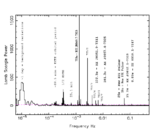
Figure 41: Periodogram for the deep (2 day) observation shows 7 pulsars, two of which were new discoveries. From left: RX J0049.7-7323, RX J0051.9-7311, AX J0057.4-7325, XTE 51sec, XTE16.6sec, RX J0052.1-7319, 2E 0050.1-7247

One very deep observation was made at Position 4 (see Table 1). Beginning on MJD 51801.2 a total of 106.5 ksec of good time, spanning nearly 3 days was obtained. The standard analysis as described above revealed the presence of 7 pulsars, of which 2 were new discoveries. The dataset was included in the long-term lightcurves presented above. The periodogram is shown in Figure 41 with all of the 99% significant peaks labeled and identified. Because this observation spanned a very long time interval, the periodogram was calculated out to 100 ksec in order to search for hitherto undiscovered long-period pulsars. A number of features are evident at low frequencies and most of these are attributed to systematic effects related to the RXTE orbital period and residual diurnal background variations. Pulsars detected are (from left in Figure 41) RX J0049.7-7323 and several harmonics, RX J0051.9-7311, AX J0057.4-7325, XTE 51s (detected P/2 harmonic), XTE 16.6s, RX J0052.1-7319, 2E 0050.1-7247.

5 Known SMC Pulsars Not Detected With RXTE

A table of known SMC X-ray pulsars which were not detected in any of the monitoring observations despite being in the RXTE field of view at various times is provided, see Figure 4. In each case a single upper limit on the flux is quoted, based on the observation judged to be the most sensitive in terms of position, duration, and number of detectors functioning.

6 General Properties of the SMC HMXB Population.

6.1 Pulse Periods

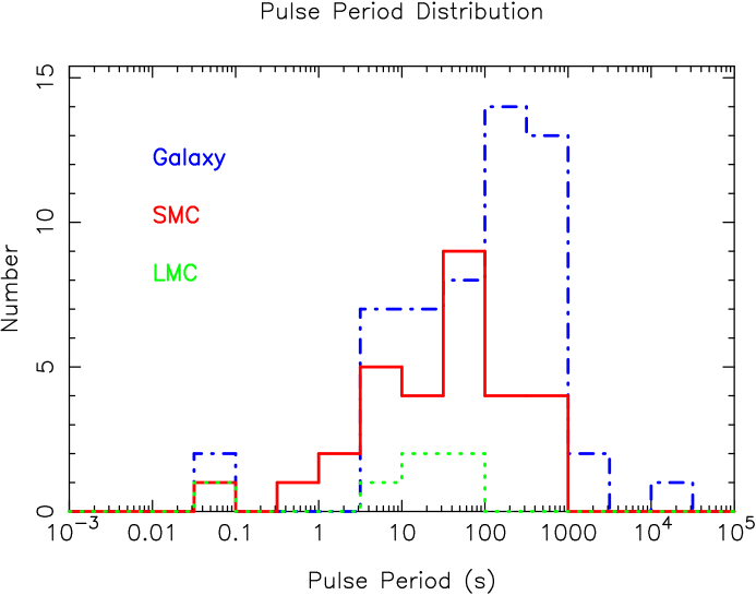
Figure 42: Distribution of pulse periods in the SMC, LMC and the Galaxy. The SMC population appears to be shifted to shorter periods, the significance of this effect is 97% according to the K-S test.

We compare the pulse period distributions for X-ray pulsars in the SMC, LMC and the Galaxy. Figure 42 shows the 3 populations binned with 2 bins per decade in period. A comparable number of pulsars are known in the SMC (30) and Galaxy (54), and a lesser number in the LMC (Liu et al, 2000; Sakano et al, 2000; Marshall et al, 2000; in’t Zand et al, 2001; Bamba et al, 2001).

The pulse periods in Figure 42 mainly occupy the 10 - few 100 s range, with the Galactic population skewed toward longer periods. The known range of pulse periods stretches from below 0.1s to over 1000s. We compared the Galactic and SMC populations with the Kolmogorov-Smirnov test. The K-S statistic was 0.3222, giving a probability of 0.028 that the two samples are drawn from the same population. Some caution is required in interpreting this result because the conditions under which the two samples were obtained were far from homogeneous. If one were to try to characterize typical observing conditions for the SMC pulsars the important factors would be low galactic extinction, and constant distance ($\sim$65kpc). For the Galactic pulsars the conditions are varying extinction across as much as several decades in $N_{H}$ and a wide range of distances which are uncertain by factors of 2 or more.

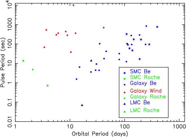
Figure 43: The $P_{pulse}/P_{orbit}$ diagram for HMXBs in the Galaxy and Magellanic Clouds, the SMC orbital periods are the candidate periods presented in this paper.

If systematic differences exist between the pulse period distributions in the two galaxies, physical causes must be disentangled from selection effects. Our results presented here tend to support the link between X-ray luminosity and pulse period. Stella et al (1986) pointed out that the maximum observed luminosity for binary X-ray pulsars is anti-correlated with $P_{pulse}$, although the results presented here suggest that the effect is weak for periods longer than a few seconds. Luminosity selection bias (against fainter long period pulsars) in our survey seems unlikely to seriously affect results. A more serious bias against long period pulsars is observation length: 3 ksec is only long enough to detect pulsars up to periods of about 750 seconds. At very short pulse periods, there is unlikely to be any luminosity bias because these sources are bright (typically several 10³⁷${\rm\thinspace erg}{\rm\thinspace s}^{-1}$). The important factor for short period pulsars is density of observing coverage because these systems rarely go into outburst. It seems unlikely that any other pulsars similar to SMC X-2 and XTE J0052-723 could have been missed because the typical duration of these outbursts is several weeks. With observations on a weekly basis at a sensitivity $\sim$10³⁶${\rm\thinspace erg}{\rm\thinspace s}^{-1}$ any such pulsars would have been detected if they lie within the field of view of the PCA. XTE J0052-723 was easily detected at a collimator response of just 0.2. A look at the Corbet diagram for Galactic and SMC pulsars (Figure 43) reveals that the cause of the discrepancy in pulse period distributions is in fact the predominance of Be/X-ray binaries in the SMC.

Our luminosity sensitivity of $\sim$10³⁶${\rm\thinspace erg}{\rm\thinspace s}^{-1}$ may be converted into an approximate pulse period detection threshold. Stella et al (1986) found an inverse correlation between pulse period and maximum X-ray luminosity. From Figure 2 of Stella et al (1986) our luminosity sensitivity implies that we would be able to detect SMC pulsars with periods shorter than $\sim$1000 seconds if SMC pulsars follow the same relationship. We note that Majid et al (2004) do find a comparable relationship between maximum luminosity and pulse period for the SMC and Galactic sources.

For Galactic HMXBs, a significant fraction of long period pulsars are accreting from the winds of supergiant companions. These systems, although variable, are persistent which makes them much easier to detect than transient Be star systems. In spite of this, none of the SMC pulsars under discussion here has the characteristics of a supergiant wind-fed binary. Therefore, one contribution to the difference between the Galactic and SMC pulse period distributions is the apparent lack of supergiant wind-accretion pulsars in the SMC.

6.2 Orbital Periods

Transient Be star X-ray pulsars exhibit two types of outbursts (e.g. Bildsten et al, 1997). Type I outbursts recur, when a system is in an active state, on the orbital period of the system. Activity is confined to limited orbital phases around the time of periastron passage. This activity pattern is the most common type of outburst. In addition, Type II (giant) outbursts may also occur where the X-ray luminosity is much larger and is not modulated on the orbital period. Our observations of SMC pulsars (over a timescale very much longer than the expected orbital periods) shows detections of repeat outbursts in 10 sources. Under the assumption that many of these are the more common Type I outbursts, these should allow the estimation of orbital periods for several systems.

Candidate orbital periods and their uncertainties are listed in Table 5. Under the widely discussed “standard” model of Be/X-ray binaries (e.g. Negueruela, 1998), it is expected that Type I outbursts will occur periodically as the neutron star’s eccentric orbit intercepts the Be star’s circumstellar disk, while type II outbursts are triggered by large-scale enhancements in the disk. Orbital periods for the SMC pulsars and for all known Galactic HMXB systems are shown in Figure 43, an updated version of the $P_{spin}/P_{orbit}$ diagram (Corbet, 1986). Uncertainties in $P_{orbit}$ are indicated, uncertainties in $P_{pulse}$ are smaller than the plot symbols.

The $P_{spin}/P_{orbit}$ diagram demonstrates that X-ray pulsars with massive companions display three different correlations between their pulse and orbital periods. These correlations have been successfully explained by Corbet (1986) in terms of the specific mode of mass transfer occurring in the binary. Different regions of the diagram are populated by systems undergoing steady wind-fed accretion, Roche lobe overflow, and transient (often periodic) accretion as is the case for Be systems. A powerful feature of the Corbet diagram is that the optical counterpart to an HMXB can be predicted to a high degree of confidence if only the timing parameters are known. Optical counterparts for around half of the currently known SMC pulsars have been identified and classified. The similarity of the X-ray properties of virtually all SMC pulsars (excepting SMC X-1) suggest the unidentified sources are also Be/X-ray binaries. In summary this evidence comprises: (1) the transient nature of the X-ray emission, (2) the typical luminosities and (3) the spectral parameters. The picture established from X-ray observations is supported by the optical identifications all of which are Be, excluding SMC X-1 which seems to be the lone example of its class. There are 32 HMXBs in the Galaxy for which both orbital and pulse periods have been reported, and 2 in the LMC (Liu et al, 2000; in’t Zand et al, 2001b; Delgado-Marti et al, 2001; in’t Zand et al, 2001). In Figure 43 color coding used to signify the 3 types of high mass accreting systems. Square, triangle, and star symbols indicate Galactic, LMC and SMC sources respectively.

All 8 of the newly determined candidate orbital periods for SMC pulsars lie in the upper half of the Be distribution as defined by the Galactic systems. Despite the pulse period distribution being weighted (although weakly) in the opposite direction. There is no characteristic of our RXTE observing strategy that would be expected to cause a bias toward finding pulsars with such long orbital periods, although the weekly sampling makes orbital periods below about 14 days difficult to measure. The apparent lack of short orbital periods for the SMC population is instead due to the small number of pulsars detected with pulse periods below $\sim$10s. For periods approaching 1 second, the minimum accretion-driven luminosity for a 10¹² G neutron star is close to the Eddington limit. So fast spinning pulsars are expected to spend the majority of the time in the centrifugal inhibition regime (if they are in Be systems). Thus unless a large dense Be star disk is continuously present, regular type I outbursts cannot occur. For such systems the orbital period can only be determined from pulse timing analysis or monitoring of the optical counterpart.

7 Spectral Parameters

HMXB spectra are in general characterized by a single power law, modified by absorption at low energy and an exponential cut-off at high energy (e.g. White et al, 1983). In systems where a cyclotron scattering resonance feature has been seen, which provides a measurement of the neutron star magnetic field strength, the spectral cutoff energy is found to be correlated with cyclotron energy (e.g. Makishima & Mihara, 1992; Coburn et al, 2002). Measurements of spectral cutoffs thus provide at least estimates of the magnetic field strength. A fluorescence line is also often seen at 6.4 keV corresponding to the iron K line from relatively cool material (Nagase, 1989).

For each bright pulsar observed during the SMC monitoring, a spectral fit was performed for at least one detection. Spectra were only extracted when no other pulsar was active, to avoid cross-contamination. The resulting spectral parameters given in Table 5 show values consistent with those exhibited by Galactic sources (White et al, 1983).

Iron lines were detected in most SMC pulsars: typical line widths were around 0.5 keV and the line strengths ($\sigma$) were correlated with overall luminosity. One exception to the above was XTE J0055-724 (period 59 s) which was X-ray bright but showed no trace of an iron K line. Three sources stand out as having peculiar features at the high energy end of their PCA spectra. The 74.7s, 172.4s and 323s pulsars all show very steep cutoffs although their spectral indices below the cut-off are not unusual. In addition these fits are not good representations of the observed spectra above the cutoff and the residuals show the possible presence of either a deep absorption feature around 20 keV or an emission feature at slightly lower energy. The two most notable of these are also the most frequently active sources in the SMC. The 172.4s and 323s pulsars were found to exhibit at least 5 and 7 outburst respectively. The pulsed-lightcurves presented in Section 3 show that the situation with these two sources is complex and there may be faint pulsations emitted at scattered times not clearly correlated with orbital phase. This interpretation of the pulsed lightcurves could imply that the pulsars are not being centrifugally inhibited at low accretion rates. Such a situation would be consistent with a lower value for the magnetic field which would be expected to reveal itself as unusually low energy cyclotron lines in the X-ray spectrum.

8 The Spatial Distribution of HMXB in the SMC

HMXB provide tracers of recent star formation activity because they are short lived, make an appearance very soon in the evolution of a star forming region, and are of course highly conspicuous. It has been noted that many X-ray pulsars discovered in the Galaxy are concentrated in the nearby “5 kpc arm”, a region identified by radio, IR, and CO molecular line emissions (Hayakawa et al, 1977). Six pulsars discovered with the Ginga satellite are known in this region and all are transient sources having the X-ray characteristics of Be systems. Spiral arms in galaxies are well known to harbor star forming regions and in fact such regions account for the majority of star formation within galaxies. The work of Maeder et al (1999) proposes that the ratio of Be to normal B type stars is higher in the SMC than in the Galaxy, although this was based on observations of certain SMC clusters which are probably not representative of the SMC as a whole. A promising line of inquiry would be to carry out a similar survey concentrating on comparing the regions harboring concentrations of HMXB. In order to identify the regions to observe, a large number of HMXB are needed for significant clustering to become apparent. Be stars are themselves relatively conspicuous objects from their photometric colors, and their place as the most common optical counterpart in HMXB undoubtedly has strong implications for the preferred channel for massive binary star evolution.

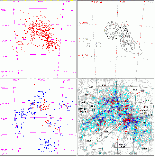
Figure 44: Spatial distributions (clockwise from top left) 1. Emission line stars, 2. Isodensity contours for stars aged 8-12.2 My, 3. Neutral hydrogen map, with positions of X-ray pulsars superimposed, 4. ROSAT X-ray Sources, blue +’s= PSPC, red +’s= HRI point sources. Credits: 1. ALADIN/Meyssonnier & Azzopardi (1993), 2. adapted from Maragoudaki et al (2001), 3. HI map adapted from Stanimirovic et al (1999), 4. ALADIN/Haberl et al (2000); Sasaki & Haberl (2000)

Recent optical surveys of the SMC (Zaritsky et al, 2000; Cioni et al, 2000; Maragoudaki et al, 2001) show that the young stellar population is concentrated into distinct structures. 30 X-ray pulsars have been identified in the SMC, the majority with positions to the  arcminute level. These positions are plotted in Figure 44 and can be compared with the distributions of other SMC constituents. Neutral hydrogen is a natural galactic constituent to compare with the HMXB distribution because large concentrations of hydrogen are a necessary precursor to star formation. Figure 44 panel 3 shows the HI density distribution as mapped by Stanimirovic et al (1999), superimposed are the positions of all the SMC pulsar with accurately known positions. Maragoudaki et al (2001) produced isodensity contour maps of the SMC showing the spatial distributions of stars of different ages. Perhaps the most interesting panel from the point of view of HMXBs is the distribution of stars whose age is comparable to the evolutionary timescale for HMXB formation. The isochrone map for stars aged 8 - 12.2 My is reproduced here in Figure 44 panel 2. A catalog of emission-line stars in the SMC has been compiled by Meyssonnier & Azzopardi (1993) based on an objective-prism survey. The catalog was searched for all objects with a positively detected H$\alpha$ emission-line, in a 5 degree wide field centered on the SMC, and the results are plotted in Figure 44 panel 1. The final population distribution plotted here is the X-ray source population as seen by ROSAT with the PSPC and HRI. The PSPC catalog is larger due to greater sensitivity however the HRI catalog gives the possibility to restrict the search to point-sources only. This distinction enables at least an approximate restriction to a sample of HMXB. There is some observing bias surrounding the ROSAT distribution because the 5$\arcdeg\times$5$\arcdeg$ field was not uniformly observed by either ROSAT instrument, it appears that the main body of the SMC was evenly covered while the two apparent clusters around (00^h 40^m, -72^∘) and (01^h 20^m, -75^∘) are due to two particular pointings. The cluster of sources in the “wing” is real.

Looking at Figure 44 it is apparent that there is a close correlation between the spatial distributions of the 5 populations. The SMC bar and wing are clearly marked out by the clustering of X-ray sources, emission-line stars, young stars and HI.

9 Summary

The SMC is an intriguing galaxy because of its surprisingly high abundance of X-ray pulsars. The X-ray binary population of the SMC shows important differences from the LMC and the Galaxy. The SMC appears to have been chemically isolated from the Galaxy and has been sculpted by gravitational and hydrodynamic forces originating in tidal interactions with the LMC and the Galaxy. As such the SMC provides an ideal environment in which to study the effects of dynamic encounters on star formation and the evolution of the stellar population. A number of recent works have revealed patterns in the spatial distributions of different aged stellar populations, and this evidence can be used to constrain various models of stellar evolution and structure formation. The large population of pulsars provides both a probe of the star formation and an ideal sample to investigate the general properties of HMXB.

Appendix A Catalog of Sources Detected

Parameters are summarized here for each pulsar detected during the project. For every known pulsar in the SMC, name(s), position and optical counterpart can be found in Table 6. This table should be used to identify the pulsars for which detailed measurements were made during the RXTE monitoring project. Parameters determined in this work are summarized in Table 5 and concern the subset of 18 pulsars which were observed under particularly good signal to noise conditions. For these pulsars the minimum and maximum pulsed fluxes, spectral parameters, and luminosities are presented.

A complete description of the columns in Table 5 is given below:

(1) Pulse Period. All of the pulsars exhibited pulse period variations, this column lists a characteristic value.
(2) Orbital period. Measured in days by the methods described in the relevant sections of this paper.
(3) $T_{0}$ Epoch of Phase 0. Orbital period zero point, where phase zero is taken to correspond with peak X-ray emission.
(4) Minimum pulsed flux. Units of ${\rm\thinspace counts}{\rm\thinspace PCU}^{-1}{\rm\thinspace s}^{-1}\,$. Lowest pulsed flux measured for the source at better than 99% significance. Determined from the power spectrum as described in Section 3.
(5) Maximum pulsed flux. Units of ${\rm\thinspace counts}{\rm\thinspace PCU}^{-1}{\rm\thinspace s}^{-1}\,$.
(6)-(16) Characteristic Spectral parameters. Taken from selected observations based on brightness and lack of interfering sources. Fluxes are the absorbed values in 10^-11${\rm\thinspace erg}{\rm\thinspace cm}^{-2}{\rm\thinspace s}^{-1}\,$. With the exception of (L_x) the values have not been corrected for collimator response or distance to the SMC.
(9) Absorption column density for neutral hydrogen in units of 10²²cm^-2
(14) Reduced $\chi^{2}$ for the fit. Fits were performed over the range 3 - 20 keV.
(15) Collimator response for the pulsar in the observation from which the spectral fit was performed. Numbers in parentheses are the pointing positions. Both parameters refer to Table 1.
(16) Luminosity in units of 10³⁷ erg s^-1 The unabsorbed source luminosity assuming a distance of 65kpc after correction for collimator response. The 2-10 keV luminosity is given to facilitate comparison with results from other missions.

Figure 3: SMC X-2 pulsed flux history. Top panel: pulse amplitude in ${\rm\thinspace counts}{\rm\thinspace PCU}^{-1}{\rm\thinspace s}^{-1}\,$, filled symbols indicate $>$99% detection significance. Middle panel: pulse period and uncertainty for positive detections. Bottom panel: detection significance, squares= blind search, circles= assuming prior knowledge of the pulse period.

Figure 5: XTE J0052-723 pulsed flux history. Top panel: pulse amplitude in ${\rm\thinspace counts}{\rm\thinspace PCU}^{-1}{\rm\thinspace s}^{-1}\,$, filled symbols indicate $>$99% detection significance. Middle panel: pulse period and uncertainty for positive detections. Bottom panel: detection significance, squares= blind search, circles= assuming prior knowledge of the pulse period.

Figure 6: 2E 0050.1-7247, XTE 8.88, pulsed flux and period history.

Figure 7: Pulse profile for the 8.88s pulsar 2E 0050.1-7247.

Figure 8: XTE 16.6s, (may be AX J0058-720) pulsed flux and period history.

Figure 9: Pulse profile for the XTE 16.6 pulsar (may be AX J0058-720), flux is in counts per PCU per second.

Figure 10: Pulse profile for the 31s pulsar XTE J0111.2-7317

Figure 11: XTE 46.6 (1WGA J0053.8-7226) pulsed flux and period history.

Figure 12: XTE 46.6. Folded pulsed flux lightcurve at a period of 138 days. Note the feature at a phase of 0.5 which is possibly also visible in the unfolded lightcurve.

Figure 13: Pulse profile (3-10 keV) for the 46.6 second pulsar 1WGA J0053.8-7226.

Figure 14: XTE J0055-724. Pulsed flux and period history.

Figure 15: XTE J0055-724 pulsed flux lightcurve folded at 123 day orbital period.

Figure 16: Pulse profile of the 59 s pulsar XTE J0055-724

Figure 17: AX J0049-729. Pulsed flux and period history.

Figure 18: Pulse profile of the 74s pulsar AX J0049-729

Figure 19: AX J0049-729. 99% significance detections of the 74s pulsar folded at 642$\pm$59 days.

Figure 20: XTE J0052-725. Pulsed flux and period history.

Figure 21: XTE 91s (AX J0051-722). Pulsed flux and period history.

Figure 22: Pulsed flux lightcurve for the 91s pulsar AX J0051-722, folded at a period of 115 days

Figure 23: Pulse profile for the 91 second pulsar AX J0051-722.

Figure 24: XTE SMC95. Pulsed flux and period history.

Figure 25: Pulse profile for the 95s XTE pulsar.

Figure 26: AX J0057.4-7325. Pulsed flux and period history.

Figure 27: XTE J0054-720. Pulsed flux and period history.

Figure 28: Folded 99% detections of the 169s pulsar XTE J0054-720 at a period of 224 days.

Figure 29: Pulse profile for XTE J0054-720 (169s)

Figure 30: AX J0051.6-7311. Pulsed flux and period history.

Figure 31: Lightcurve for AX J0051.6-7311, 99% significance detections (MJD 51600-52100) folded at a period of 67d.

Figure 32: Pulse profile for the 172.4 second pulsar AX J0051.6-7311

Figure 33: RX J0050.8-7316. Pulsed flux and period history.

Figure 34: Folded lightcurve for RX J0050.8-7316 (323s) at a period of 109 days. The 6 brightest points are from observations at position 1, the rest are from position 5. (See Table 1)

Figure 35: Pulse profile for the 323s pulsar RX J0050.8-7316

Figure 36: AX J0103-722. Pulsed flux and period history.

Figure 37: Pulse profile for the 348s pulsar AX J0103-722

Figure 38: RX J0101.5-7211. Pulsed flux and period history.

Figure 39: AX J0049.4-7323. Pulsed flux and period history. Two outbursts exceeding 3$\times 10^{37}$ ${\rm\thinspace erg}{\rm\thinspace s}^{-1}$ are separated by 396 days.

Figure 40: Pulse profile for the 751s pulsar AX J0049.4-7323.

.

Table 1: Pointing Positions for SMC Monitoring.

Position	$N_{obs}(N_{sec})$	Dates (MJD)	$RA(\arcdeg)$	$Dec(\arcdeg)$
1a	9 (13)	50779 - 50802	13.033	-72.429
1b	1 (1)	50825	12.767	-72.229
1c	18 (31)	50833 - 51115	13.728	-72.445
1	41 (54)	51186 - 51555	13.471	-72.445
2	4 (6)	51198 - 51326	16.25	-72.1
3	3 (4)	51220 - 51310	18.75	-73.1
4	6 (4)	51348 - 51417	12.686	-73.268
5	45 (70)	51560 - 52333	12.5	-73.1

Table 2: RXTE PCA Pointed Observations of SMC X-2.

Obs.	Date	Period	Flux	Pulsed Flux
	(2000)	(sec)	${\rm\thinspace counts}{\rm\thinspace PCU}^{-1}{\rm\thinspace s}^{-1}\,$	${\rm\thinspace counts}{\rm\thinspace PCU}^{-1}{\rm\thinspace s}^{-1}\,$
1†	Jan 24	2.3728(1)	0.03	0.16
2	Jan 30	2.37210(5)	10.04	2.91
3	Feb 6	2.3717(1)	11.32	1.34
4	Feb 12	2.37281(1)	16.15	1.44
5	Feb 18	2.371815(5)	26.49	11.97
6	Feb 26	2.371787(5)	25.23	7.99
7	Apr 6	2.372217(5)	8.45	1.96
8a	Apr 12-13	2.37157(1)	7.14	1.86
8b∗	Apr 12		5.2	-
9	Apr 18	2.3711(1)	7.02	1.62
10∗	Apr 22-23	2.371859(5)	3.23	1.19

Table 3: Spectral fits for SMC X-2

Obs	5	8b	10
$N_{H}\times 10^{22}$	1.6 $\pm$ 0.3	1.6$\pm$0.8	3.3$\pm$0.6
$\alpha$	1.17$\pm$0.02	0.70$\pm$0.04	1.0$\pm$0.03
$E_{c}$	12.4$\pm$1
$E_{f}$	50$\pm$12
$\sigma Fe$	0.8$\pm$0.2
norm $Fe$	(2.9$\pm$1)$\times 10^{-10}$
$flux_{2-10}$	1.5$\times 10^{-10}$	6.93$\times 10^{-11}$	5.71$\times 10^{-11}$
$flux_{10-20}$	1.6$\times 10^{-10}$
$L_{X}$	4.4$\times 10^{38}$
$\chi_{\nu}{{}^{2}}$	1.25	1.52	1.12

Table 4: Pulsars not detected with RXTE.

Pulsar	Period (s)	${\rm\thinspace counts}{\rm\thinspace PCU}^{-1}{\rm\thinspace s}^{-1}\,$	Ref.
RX J0059.2-7138	2.8	$<$0.40	Hughes (1994)
AX J0105-722	3.34	$<$0.16	Yokogawa et al (1998)
AX J0049-732	9.13	$<$0.10	Imanishi et al (1998)
RX J0117.6-7330	22	$<$0.29	Charles et al (1996)
AX J0058-7203	280	$<$0.17	Yokogawa et al (1998a)

Table 5: Measured X-ray properties for SMC pulsars.

Ppulse	Porbit	T0	Fpmin	Fpmax	f${}_{X}^{2-10}$	f${}_{X}^{10-20}$	$\alpha$	nH	Ecut	Efold	$\sigma$Fe	EW(Fe)	$\chi^{2}$	R(pos)	L${}_{x}^{2-10}$
s	days	MJD							keV	keV	eV	eV
2.374			1.29	12.41	14.95	16.0	1.17	1.63	12.4	50	0.75	148	1.25	0.33 (5)	21.5
4.78			1.63	2.29	13.47	9.08	1.7	2.5	15	12	0.78	196	0.86	1 (*)	7.241
16.6	1189$\pm$18	51393	0.27	0.97
31.0			-	0.90	8.905	10.99	0.968	1.46	12.23	29	0.42	122	0.99	0.67 (3)	6.845
46.6	2139$\pm$6	50779	0.19	0.92
51
58.97	3123$\pm$1	50841	0.18	2.76	7.3677	5.84	1.26	2.9	7.6	18	no	-	0.6	0.98 (1c)	4.257
74.7	4642$\pm$59	52078	0.24	1.96	2.157	1.90	1.219	1.395	16.24	2.5	0.54	182	0.61	0.75 (5)	1.491
82.4			0.24	1.90
91.1	5115$\pm$5	50784	0.28	1.92
95s	6283$\pm$8	51248	0.39	0.89	2.375	2.03	1.26	0.72	15	12	weak	-	0.6	1 (1*)	1.2
101.4			0.18	1.33
169	7200$\pm$40	50800	0.22	1.88
172.4	8147$\pm$24	51694	0.08	1.29	1.005	0.55	1.251	0.04	12	5	0.51	536	0.83	0.86 (5)	0.5563
323	9109$\pm$18	51651	0.06	1.67	1.95	1.46	1.45	4.6	13	7	0.56	264	0.69	0.83 (5)	1.1137
343			0.35	1.45
455			0.37	0.88
755	10396$\pm$5	51800	0.27	3.20	3.14	2.04	1.55	1.8	12.16	14	0.6	330	0.85	0.71 (5)	2.387

Note. — Column $N_{obs}(N_{sec})$ indicates the number of whole observations followed by the number of separate sections into which these were split for analysis. Coordinates are epoch 2000.

Note. — ^∗ Observations centered on SMC X-2, previously appeared in Corbet et al (2001) Table 1 as numbers 2 & 3. All other observations were centered on RA = $0^{h}50^{m}$, Dec = $-73\arcdeg$6′. †Observation 1 has unreliable flux calibration due to a telemetry error.

Note. — Units are keV for $E_{c}$, $E_{f}$, $\sigma Fe$. Flux units ${\rm\thinspace erg}{\rm\thinspace cm}^{-2}{\rm\thinspace s}^{-1}\,$. Luminosity units (unabsorbed) erg s^-1 at 65 kpc, collimator response 0.33. Parameters for observations 8b and 10 are taken from Corbet et al (2001).

Note. — Upper limits on the RXTE PCA pulsed-flux for 5 previously known Be/X-ray pulsars, which were not detected during our survey.

Note. — Explanation of columns is given in the text.

Notes on period determination:

(1) Period determined from 5 evenly spaced faint outbursts.

(2) From 6 outbursts. (3) From 4 very bright and well observed outbursts. (4) From 3 outbursts, 1 bright, 2 faint. (5) 2 bright outbursts and up to 6 faint ones. (6) From 2 bright outbursts. (7) Up to 4 faint outbursts, uncertain. (8) Numerous detections. Period determined from a string of 6 evenly spaced brighter outbursts. (9) Many detections with weak pattern. (10) 2 very bright outbursts.

Table 6: List of X-ray Pulsars in the SMC.

Pulse Period (s)	RA	Dec	Optical Counterpart	Name(s)
0.087	00 42 35	-73 40 30		AX J0043-737
0.716	01 17 05.1	-73 26 35	B1Iab	SMC X-1
2.374	00 54 33	-73 41 04	B1.5Ve	SMC X-2
2.8	00 59 12.9	-71 38 50	B0III-Ve	RX J0059.2-7138
3.34	01 05 06	-72 11 08	-	AX J0105-722 ( RX J0105.3-7210?)
4.782	00 53 07	-72 17 24	B0V-B1Ve	XTE J0052-723
7.77	(AO7 Position A)		-	XTE 7.77
8.88	00 54 28.7	-72 45 37	B1e	2E 0050.1-7247
9.13	00 49 23	-73 12 38	-	AX J0049-732
15.3	00 52 15.5	-73 19 14	Be	RX J0052.1-7319
16.6	00 51 51.2	-73 10 32	-	XTE
22.07	01 17 40	-73 30 48	B1-2 III-Ve	RX J0117.6-7330
31.0	01 11 14.5	-73 16 50	Be	XTE J0111.2-7317
46.4	(Positions 4 & 5)		-	XTE 46.4
46.6	00 53 56	-72 26 54	Be	XTE 1WGA J0053.8-7226
51	(Positions 4 & 5)		-	XTE 51
58.97	00 55 00	-72 25 38	Be	XTE J0055-724, 1SAX J0054.9-7226, 2E 0053.2-7242
74.7	00 49 00	-72 51 40	Be	XTE nameless, AX J0049-729, RX J0049.1-7250
82.4	13.23	-72.23	-	XTE 82.4
89	(AO7 Position A)		-	XTE 89
91.1	00 51 11	-72 14 01	Be	XTE, AX J0051-722
95.2	AO4/5 POS1		-	XTE SMC95
101.4	00 57 27	-73 25 31	-	AX J0057.4-7325
169.3	00 54.6	-72 04	Be	XTE J0054-720 AX J0052.9-7157 RXJ0052.9-7158
172.4	00 51 38	-73 11 01	Be	AX J0051.6-7311
280.4	00 57 58	-72 02 56		AX J0058-720
323	00 50 47	-73 15 51	Be	ASCA/ROSAT RX J0050.8-7316
348/343	01 03 15	-72 09 01	Be	AX J0103-722 1SAX J0103.2-7209 2E 0101.5-7225
455+-2	01 01 21	-72 11 18	Be	RX J0101.3-7211
755.5	00 49 33	-73 23 23		RX J0049.7-7323 AX J0049.4-7323

Pulsars in this table are ordered by pulse period. Spectral type of the optical counterpart is given if known. Where the source position is not accurately known, we give the monitoring positions (see Table  1) in which the pulsar was detected.

Table 7: PCA collimator response $R$ for all SMC pulsars with well known positions.

Pulsar	RA	Dec	Pos 1	Pos 2	Pos 3	Pos 4	Pos 5	Pos 1a	Pos 1b	Pos 1c
0.087s	10.65	-73.68				0.29	0.22
0.716s	19.25	-73.44			0.63
2.374s	13.64	-73.68				0.50	0.33
2.8s	14.80	-71.65	0.10	0.36					0.14	0.14
3.34s	16.28	-72.19	0.11	0.91						0.18
4.78s	13.08	-72.33	0.84				0.21	0.90	0.86	0.77
8.88s	13.62	-72.76	0.68			0.42	0.53	0.63	0.41	0.68
9.13s	12.35	-73.21	0.16			0.89	0.88	0.19		0.13
15.3s	13.06	-73.32	0.12			0.88	0.73	0.11		0.10
16.66s	12.96	-73.18	0.25			0.88	0.85	0.25		0.23
22.07s	19.42	-73.51			0.54
31.0s	17.81	-73.28			0.67
46.6s	13.48	-72.45	1.00			0.15	0.29	0.86	0.69	0.93
58.97s	13.75	-72.43	0.91	0.17		0.10	0.23	0.78	0.64	0.98
74.7s	12.25	-72.86	0.45			0.57	0.75	0.51	0.35	0.39
82.4s	13.23	-72.55	0.87			0.26	0.41	0.87	0.65	0.82
91.1s	12.80	-72.23	0.71				0.13	0.79	0.99	0.65
101.4s	14.36	-73.43				0.49	0.37
169s	13.65	-72.07	0.62	0.20				0.59	0.68	0.62
172.4s	12.91	-73.18	0.24			0.89	0.86	0.24		0.22
280.4s	14.49	-72.15	0.57	0.46				0.48	0.47	0.63
323s	12.70	-73.26	0.15			1.00	0.83	0.16		0.13
343s	15.81	-72.15	0.23	0.86				0.11		0.30
455s	15.34	-72.19	0.38	0.71				0.26	0.21	0.45
755s	12.39	-73.39				0.85	0.71

The $RA$ & $Dec$ (J2000) for each pointing position are given in Table 1. Blank entries indicate that the source was not in the field of view. These values were used in the reduction of pulsar monitoring data.

References

- Bamba et al (2001) Bamba A., Yokogawa J., Ueno M., Koyama K., Yamauchi S., 2001, PASJ, 53, 1179
- Bildsten et al (1997) Bildsten, L., Chakrabarty, D., Chiu, J., Finger, M. H., Koh D. T., Nelson, R. W., Prince T. A., Rubin B. C., Scott D. M., Stollberg M., Vaughan B. A., Wilson C. A., Wilson R. B., 1997, ApJS, 113, 367
- Bildsten (1998) Bildsten L., 1998, “The Angular Momentum of Accreting Neutron Stars”, in “Accretion Processes in Astrophysical Systems: Some Like it Hot!”, AIP Conference Proceedings 431, ed. S.S. Holt & T.R. Kallman, pp. 299-308
- Buckley et al (2001) Buckley, D. A. H., Coe, M. J., Stevens, J. B., van der Heyden, K., Angelini, L., White, N., Giommi, P., 2001 MNRAS, 320, 281
- Chakrabarty et al (1998a) Chakrabarty D., Levine A. M., Clarke G. W., Takeshima T., 1998, IAUC, 7048
- Charles et al (1996) Charles P. A., Southwell K. A., O’Donoghue D., 1996, IAUC, 6305
- Cioni et al (2000) Cioni M. R. L., Habing H. J., & Israel F. P., 2000, A&A, 358, L9
- Clarke et al (1978) Clarke G., Doxsey R., Li F., Jernigan J. G., 1978, ApJ, 221, L37
- Coburn et al (2002) Coburn W., Heindl W. A., Rothschild R. E., Gruber D. E., Kreykenbohm I., Wilms J., Kretschmar P., & Staubert R., 2002, ApJ, 580, 394
- Coe et al (1998) Coe M. J., Buckley, D. A. H., Charles P. A., Southwell K. A., Stevens J. B., 1998, MNRAS, 293, 43
- Coe & Orosz (2000) Coe M. J., & Orosz J. A., 2000, MNRAS, 311, 169
- Cowley et al (1997) Cowley A. P., Schmidtke P. C., McGrath T.K., Ponder A. L., Fertig M. R., Hutchings J. B., & Crampton D., 1997, PASP, 109, 21
- Cowley & Schmitdke (1997) Cowley A. P., & Scmidtke P. C., 2003, AJ, 126, 2949
- Coe et al (2002) Coe M. J., Haigh N. J., Laycock S., Negueruela I., Kaiser C. R., 2002, MNRAS, 332, 473
- Corbet (1986) Corbet R. H. D., 1986, MNRAS, 220, 1047
- Corbet et al (1998) Corbet R. H. D., Marshall F. E., Lochner J. C., Ozaki M., Ueda Y., 1998, IAUC 6803
- Corbet et al (2001) Corbet R. H. D., Marshall, F. E., Coe, M. J., Laycock, S., Handler, G., 2001 ApJ, 548, L41
- Corbet et al (2002) Corbet R.; Markwardt C. B. Marshall F. E., Laycock S., Coe M. J., 2002, IAUC 7932
- Delgado-Marti et al (2001) Delgado-Martí H., Levine A. M., Pfahl E., & Rappaport S. A., 2001, ApJ, 546, 455
- Edge & Coe (2003) Edge W., Coe M. J., 2003, MNRAS, 338, 428
- Ghosh & Lamb (1979) Ghosh P. & Lamb F. K., 1979, ApJ, 232, 259
- Haberl et al (2000) Haberl F., Filipovic M. D., Pietsch W., Kahabka P., 2000, A&A, 141, 41
- Hayakawa et al (1977) Hayakawa S., Ito K., Matsumoto T., & Uyama K., 1977, A&A, 58, 325
- Hughes (1994) Hughes J. P., 1994, ApJ, 427, L25
- Imanishi et al (1998) Imanishi K., Yokogawa J., & Koyama, K. 1998, IAUC, 7040
- Imanishi et al (1999) Imanishi K., Yokogawa J., Tsujimoto M., & Koyama K., 1999, PASJ, 51, L15
- in’t Zand et al (2001) in’t Zand J. J. M., Swank J., Corbet R. H. D., Markwardt C. B., 2001, A&A, 380, L26
- in’t Zand et al (2001b) in’t Zand J. J. M., Corbet R. H. D., Marshall F. E., 2001b, ApJ, 553, L165
- Jahoda et al (1996) Jahoda K., Swank J. H., Stark M. J., Strohmayer T., Zhang W., Morgan E. H., 1996, Proc. SPIE, 2808, 59
- Kahabka & Pietsch (1998) Kahabka P., Pietsch W., 1998, IAUC 6840
- Kovacs (1980) Kovacs G., 1980, Ap&SS, 69, 485
- Lamb et al (2002) Lamb R. C., Macomb D. J., Prince T. A., Majid W. A. 2001, ApJ, 567, L129
- Laycock et al (2002) Laycock S., Corbet R. H. D., Perrodin D., Coe M. J., Marshall F. E., Markwardt C., 2002, A&A, 385, 464
- Laycock et al (2003) Laycock S., Corbet R. H. D., Coe M. J., Marshall F. E., Markwardt C., Edge W. R., 2003, MNRAS, 339, 435
- Liu et al (2000) Liu Q. Z., van Paradijs J., & van den Heuvel E. P. J, 2000, A&A, 147, 25
- Lochner et al (1998a) Lochner J. C., Marshall F. E., Whitlock L. A., Brandt N., 1998, IAUC 6814
- Lochner (1998) Lochner J. C., 1998, IAUC 6858
- Lochner (1998) Lochner J. C., 1998, IAUC 7007
- Lochner et al (1999) Lochner J. C., Whitlock L. A., Corbet R. H. D., Marshall F. E., 1999, HEAD, BAAS, 31, 742
- Macomb et al (1999) Macomb D. J., Finger M. H., Harmon B. A., Lamb R. C., Prince T. A., 1999, ApJ, 518, L99
- Maeder et al (1999) Maeder, A., Grebel, E. K., & Mermilliod, J. C., 1999, A&A, 346, 456
- Makishima & Mihara (1992) Makishima, K. & Mihara, T. 1992, in Proc. 28th Yamada Conf.,Frontiers of X-ray Astronomy, ed. Y. Tanaka & K. Koyama (Tokyo: Universal Academy Press), 23
- Majid et al (2004) Majid, W.A., Lamb, R.C., Macomb, D.J., 2004, ApJ, 609, 133
- Maragoudaki et al (2001) Maragoudaki F., Kontizas M. Morgan D. H., Kontizas E., Dapergolas A., Livanou E., 2001, A&A, 379, 864
- Marshall et al (1997) Marshall F. E., Lochner J. C., Takeshima T., 1997, IAUC 6777
- Marshall et al (1998) Marshall F. E., Lochner J. C., Santangelo A., Cusuamo G., Israel G. L., dal Fiume D., Orladini M., Frontera F., Parmar A. N., Corbet R. H. D., 1998, IAUC 6818
- Marshall et al (2000) Marshall F. E., Takeshima T., in’t Zand J., 2000, IAUC 7363
- Meyssonnier & Azzopardi (1993) Meyssonnier N., & Azzopardi, M., 1993, A&A, 102, 451
- Murdin et al (1993) Murdin P., Morton D. C., Thomas R. M., 1979, MNRAS, 186, 43
- Nagase (1989) Nagase F., 1989, PASJ, 41, 1
- Negueruela (1998) Negueruela I., 1998, A&A, 338, 505
- Press & Rybicki (1989) Press W. H., Rybicki G. B., 1989, ApJ, 338, 277
- Press et al (1993) Press W. H., Teukolsky S. A., Vetterling W. T., Flannery B. P., 1993, Numerical Recipies in Fortran 2nd Ed., Cambridge University Press
- Sakano et al (2000) Sakano, M., Torii, K., Koyama K., Maeda Y., Yamauchi S., 2000, PASJ, 52, 1141
- Sasaki & Haberl (2000) Sasaki M., Haberl F., 2000, A&A, 147, 75
- Scargle (1982) Scargle J. D., 1982, ApJ, 263, 835
- Schmitdke et al (2004) Scmidtke P. C., Cowley A. P., Levenson L., Sweet K., 2005, AJ, 126, 2949
- Stanimirovic et al (1999) Stanimirovic S., Staveley-Smith L., Dickey J. M., Sault R. J., Snowden S. L., 1999, MNRAS, 302, 417
- Stellingwerf (1978) Stellingwerf R. F., 1978, ApJ, 224, 953
- Stella et al (1986) Stella, L., White, N. E., & Rosner, R., 1986, ApJ, 308, 669
- Stevens et al (1999) Stevens J. B., Coe., M. J., Buckley D. A. H., 1999, MNRAS, 309, 421
- Torii et al (2000a) Torii K., Yokogawa J., Imanishi K., & Koyama K., 2000, IAUC 7428
- Ueno et al (2000b) Ueno M., Yokogawa J., Imanishi K., & Koyama K., 2000, IAUC 7442
- White et al (1983) White N. E, Swank J. H., Holt S. S., 1983, ApJ, 263, 277
- Wilson et al (1998) Wilson C. A., Finger M. H., 1998, IAUC 7048
- Yokogawa et al (1998) Yokogawa J., & Koyama K., 1998, IAUC 7028
- Yokogawa et al (1998a) Yokogawa J., & Koyama K., 1998, IAUC 6853
- Yokogawa et al (1999) Yokogawa J., Imanishi K., Tsujimoto, M., Kohno M., Koyama K., 1999, PASJ, 51, 547
- Yokogawa et al (2000a) Yokogawa, J., Imanishi, K., Ueno M., Koyama, K., 2000, PASJ, 52, L73
- Yokogawa et al (2001) Yokogawa J., Torii K., Kohmura T., Koyama K., 2001, PASJ, 53, 227
- Yokogawa (2002) Yokogawa J., 2002, PhD Thesis, Kyoto University, Japan
- Zaritsky et al (2000) Zaritsky D., Harris J., Grebel E. K., Thompson I. B., 2000, ApJ, 534, L53