Geometrical Constraints on Dark Energy

We explore the recently introduced statefinder parameters. After reviewing their basic properties, we calculate the statefinder parameters for a variety of cosmological models, and investigate their usefulness as a means of theoretical classification of dark energy models. We then go on to consider their use in obtaining constraints on dark energy from present and future supernovae type Ia data sets. Provided that the statefinder parameters can be extracted unambiguously from the data, they give a good visual impression of where the correct model should lie. However, it is non-trivial to extract the statefinders from the data in a model-independent way, and one of our results indicates that an expansion of the dark energy density to second order in the redshift is inadequate. Hence, while a useful theoretical and visual tool, applying the statefinders to observations is not straightforward.

1 Introduction

It is generally accepted that we live in an accelerating universe. Early indications of this fact came from the magnitude-redshift relationship of galaxies (Solheim 1966), but the reality of cosmic acceleration was not taken seriously until the magnitude-redshift relationship was measured recently using high-redshift supernovae type Ia (SNIa) as standard candles (Riess et al. 1998, Perlmutter et al. 1999). The observations can be explained by invoking a contribution to the energy density with negative pressure, the simplest possibility being Lorentz Invariant Vacuum Energy (LIVE), represented by a cosmological constant. Independent evidence for a non-standard contribution to the energy budget of the universe comes from e.g. the combination of the power spectrum of the cosmic microwave background (CMB) temperature anisotropies and large-scale structure: the position of the first peak in the CMB power spectrum is consistent with the universe having zero spatial curvature, which means that the energy density is equal to the critical density. However, several probes of the large-scale matter distribution show that the contribution of standard sources of energy density, whether luminous or dark, is only a fraction of the critical density. Thus, an extra, unknown component is needed to explain the observations (Efstathiou et al. 2002; Tegmark et al. 2004).

Several models describing an accelerated universe have been suggested. Typically, they are tested against the SNIa data on a model-by-model basis using the relationship between luminosity distance and redshift, $d_{\rm L}(z)$, defined by the model. Another popular approach is to parametrize classes of dark energy models by their prediction for the so-called equation of state $w(z)\equiv p_{\rm x}/\rho_{\rm x}$, where $p_{\rm x}$ and $\rho_{\rm x}$ are the pressure and the energy density, respectively, of the dark energy component in the model. One can then Taylor expand $w(z)$ around $z=0$. The current data allow only relatively weak constraints on the zeroth-order term $w_{0}$ to be derived. A problem with this approach is that some attempts at explaining the accelerating Universe do not involve a dark component at all, but rather propose modifications of the Friedmann equations (Deffayet 2001; Deffayet, Dvali & Gabadadze 2002; Dvali, Gabadadze & Porrati 2000; Freese & Lewis 2002; Gondolo & Freese 2003; Sahni & Shtanov 2003). Furthermore, it is possible for two different dark energy models to give the same equation of state, as discussed by Padmanabhan (2002) and Padmanabhan & Choudhury (2003).

Recently, an alternative way of classifying dark energy models using geometrical quantities was proposed (Sahni et al. 2003, Alam et al. 2003). These so-called statefinder parameters are constructed from the Hubble parameter $H(z)$ and its derivatives, and in order to extract these quantities in a model-independent way from the data, one has to parametrize $H$ in an appropriate way. This approach was investigated at length in Alam et al. (2003) using simulated data from a SNAP-type experiment. In this paper, we present a further investigation of this formalism. We generalize the formalism to universe models with spatial curvature in Section 2, and give expressions for the statefinder parameters in several specific dark energy models. In the same section, we also take a detailed look at how the statefinder parameters behave for quintessence models, and show that some of the statements about these models in Alam et al. (2003) have to be modified. In Section 3 we discuss what can be learned from current SNIa data, considering both direct $\chi^{2}$ fitting of model parameters to data, and statefinder parameters. In Section 4 we look at simulated data from an idealized SNIa survey, showing that reconstruction of the statefinder parameters from data is likely to be non-trivial. Finally, Section 5 contains our conclusions.

2 Statefinder parameters: definitions and properties

The Friedmann-Robertson-Walker models of the universe have earlier been characterized by the Hubble parameter and the deceleration parameter, which depend on the first and second derivatives of the scale factor, respectively:

$$H = \frac{\dot{a}}{a}$$ (1)

$$q = -\frac{\ddot{a}a}{\dot{a}^{2}}=-\frac{\dot{H}}{H^{2}}-1,$$ (2)

where dots denote differentiation with respect to time $t$. The proposed SNAP satellite will provide accurate determinations of the luminosity distance and redshift of more than 2000 supernovae of type Ia. These data will permit a very precise determination of $a(z)$. It will then be important to include also the third derivative of the scale factor in our characterization of different universe models.

Sahni and coworkers (Sahni et al. 2003, Alam et al. 2003) recently proposed a new pair of parameters $(r,s)$ called statefinders as a means of distinguishing between different types of dark energy. The statefinders were introduced to characterize flat universe models with cold matter (dust) and dark energy. They were defined as

$$r = \frac{\stackrel{{\scriptstyle\bf{...}}}{{a}}}{aH^{3}}=\frac{\ddot{H}}{H^{3}}+3\frac{\dot{H}}{H^{2}}+1$$ (3)

$$s = \frac{r-1}{3\left(q-\frac{1}{2}\right)}.$$ (4)

Introducing the cosmic redshift $1+z=1/a\equiv x$, we have $\dot{H}=-H^{\prime}H/a$, where $H^{\prime}=dH/dx$, the deceleration parameter is given by

$$q(x)=\frac{H^{\prime}}{H}x-1.$$ (5)

Calculating $r$, making use of $a^{\prime}=-a^{2}$, we obtain

$$r(x)=1-2\frac{H^{\prime}}{H}x+\left(\frac{H^{\prime 2}}{H^{2}}+\frac{H^{\prime\prime}}{H}\right)x^{2}.$$ (6)

The statefinder $s(x)$, for flat universe models, is then found by inserting the expressions (5) and (6) into equation (4). The generalization to non-flat models will be given in the next subsection.

The Friedmann equation takes the form

$$H^{2}=\frac{8\pi G}{3}(\rho_{\rm m}+\rho_{\rm x})-\frac{k}{a^{2}},$$ (7)

where $\rho_{\rm m}$ is the density of cold matter and $\rho_{\rm x}$ is the density of the dark energy, and $k=-1,0,1$ is the curvature parameter with $k=0$ corresponding to a spatially flat universe. The dust component is pressureless, so the equation of energy conservation implies

$$\rho_{\rm m}=\rho_{\rm m0}a^{-3}.$$ (8)

This gives for the density of dark energy:

$$\rho_{\rm x} = \rho_{\rm c}-\rho_{\rm m}-\frac{3k}{8\pi Ga^{2}}$$ (9)

$$= \frac{3}{8\pi G}(H^{2}+kx^{2}-\Omega_{\rm m0}H_{0}^{2}x^{3}),$$

where and $\Omega_{\rm m0}$ and $\Omega_{\rm x0}$ are the present densities of matter and dark energy, respectively, in units of the present critical density $\rho_{\rm c0}=3H_{0}^{2}/8\pi G$. In the following, we will use the notation $\Omega_{\rm i}\equiv 8\pi G\rho_{\rm i}(t)/H^{2}(t)$, $\Omega_{\rm i0}\equiv\Omega_{\rm i}(t=t_{0})$, where $t_{0}$ is the present age of the Universe, and also $\Omega=\sum_{\rm i}\Omega_{\rm i}$. From Friedmann’s acceleration equation

$$\frac{\ddot{a}}{a}=-\frac{4\pi G}{3}\sum_{\rm i}(\rho_{\rm i}+3p_{\rm i}),$$ (10)

where $p_{\rm i}$ is the contribution to the pressure from component i, it follows that

$$p_{\rm x}=\frac{H^{2}}{4\pi G}\left(q-\frac{\Omega}{2}\right)=\frac{3}{8\pi G}\left[\frac{1}{3}(H^{2})^{\prime}x-\frac{k}{3}x^{2}-H^{2}\right].$$ (11)

Hence, if dark energy is described by an equation of state $p_{\rm x}=w(x)\rho_{\rm x}$, we have

$$w(x)=\frac{\frac{1}{3}(H^{2})^{\prime}x-H^{2}-\frac{k}{3}x^{2}}{H^{2}+kx^{2}-H_{0}^{2}\Omega_{\rm m0}x^{3}}.$$ (12)

In the following subsections, we calculate statefinder parameters for universe models with different types of dark energy.

2.1 Models with an equation of state $p=w(z)\rho$

First we consider dark energy obeying an equation of state of the form $p_{\rm x}=w\rho_{\rm x}$, where $w$ may be time-dependent. Quintessence models (Wetterich 1988; Peebles & Ratra 1988), where the dark energy is provided by a scalar field evolving in time, fall in this category. The formalism in Sahni et al. (2003) and Alam et al. (2003) will be generalized to permit universe models with spatial curvature. Then equation (4) is generalized to

$$s=\frac{r-\Omega}{3(q-\Omega/2)},$$ (13)

where $\Omega=\Omega_{\rm m}+\Omega_{\rm x}=1-\Omega_{\rm k}$, and $\Omega_{\rm k}=-k/(a^{2}H^{2})$.

The deceleration parameter can be expressed as

$$q=\frac{1}{2}[\Omega_{\rm m}+(1+3w)\Omega_{\rm x}]=\frac{1}{2}(\Omega+3w\Omega_{\rm x}).$$ (14)

Differentiation of equation (2) together with equation (3) leads to

$$r=2q^{2}+q-\frac{\dot{q}}{H}.$$ (15)

From equation (14) we have

$$\dot{q}=\frac{1}{2}\dot{\Omega}_{\rm m}+\frac{1}{2}(1+3w)\dot{\Omega}_{\rm x}+\frac{3}{2}\dot{w}\Omega_{\rm X}.$$ (16)

Furthermore,

$$\dot{\Omega}=\frac{\dot{\rho}}{\rho_{\rm c}}-\frac{\rho}{\rho_{\rm c}^{2}}\dot{\rho}_{\rm c},$$ (17)

with

$$\dot{\rho}_{\rm c}=\frac{3H\dot{H}}{4\pi G},$$ (18)

and

$$\dot{H}=-H^{2}(1+q),$$ (19)

giving

$$\dot{\rho}_{\rm c}=-2(1+q)H\rho_{\rm c},$$ (20)

which leads to

$$\dot{\Omega}=\frac{\dot{\rho}}{\rho_{\rm c}}+2(1+q)H\Omega.$$ (21)

For cold matter, $\dot{\rho}_{\rm m}=-3H\rho_{\rm m}$, giving

$$\dot{\Omega}_{\rm m}=(2q-1)H\Omega_{\rm m},$$ (22)

and for the dark energy, $\dot{\rho}_{\rm x}=-3(1+w)H\rho_{\rm x}$, giving

$$\dot{\Omega}_{\rm x}=(2q-1-3w)H\Omega_{\rm x}.$$ (23)

Inserting equations (22) and (23) into equation (16) and the resulting expression into (15) finally leads to

$$r=\Omega_{\rm m}+\left[1+\frac{9}{2}w(1+w)\right]\Omega_{\rm x}-\frac{3}{2}\frac{\dot{w}}{H}\Omega_{\rm x}.$$ (24)

Inserting equation (24) into equation (13) gives

$$s=1+w-\frac{1}{3}\frac{\dot{w}}{wH}.$$ (25)

For a flat universe $\Omega_{\rm m}+\Omega_{\rm x}=1$ and the expression for $r$ simplifies to

$$r=1+\frac{9}{2}w(1+w)\Omega_{\rm X}-\frac{3}{2}\frac{\dot{w}}{H}\Omega_{\rm x}.$$ (26)

Note that for the case of LIVE, $w=-1=\,{\rm constant}$, and one finds $r=\Omega$, $s=0$ for all redshifts. For a model with curvature and matter only one gets $r=2q=\Omega_{\rm m}$, $s=2/3$. The same result is obtained for a flat model with matter and dark energy with a constant equation of state $w=-1/3$, which is the equation of state of a frustrated network of non-Abelian cosmic strings (Eichler 1996; Bucher & Spergel 1999). Thus, the statefinder parameters cannot distinguish between these two models. However, neither of these two model universes are favoured by the current data (for one thing, they are both decelerating), so this is probably an example of academic interest only.

For a constant $w$, and $\Omega_{\rm m0}+\Omega_{\rm x0}=1$, the $q$–$r$ plane for different values of $\Omega_{\rm x}$ and $w$ is shown in figure 1. Quintessence with $w={\rm constant}$ is called quiessence. The relation between $q$ and $r$ for flat universe models with matter+quiessence is found by eliminating $\Omega_{\rm x}$ between equation (14), with $\Omega=1$, and equation (26). This gives

$$r=3(1+w)q-\frac{1}{2}(1+3w),$$ (27)

which is the equation of the dotted straight lines in figure 1. When $\Omega_{\rm x}=1$, all models lie on the solid curve given by

$$q = \frac{3}{2}w+\frac{1}{2}$$ (28)

$$r = \frac{9}{2}w(1+w)+1,$$ (29)

or

$$r=2q^{2}+q,$$ (30)

in accordance with equation (15) since $\dot{q}=0$ for these models. This curve is the lower bound for all models with a constant $w$. For $-1\leq w\leq 0$, all matter+quiessence models will at any time fall in the sector between this curve and the $r=1$-line which corresponds to $\Lambda{\rm CDM}$. The results shown in Alam et al. (2003) seem to indicate that all matter+quintessence models will fall within this same sector as the matter+quiessence models do. However, as we will show below, this is not strictly correct.

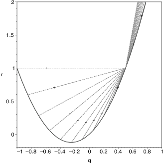
Figure 1: The $q-r$-plane for flat matter+quiessence models. The horizontal curve has $w=-1$ ($\Lambda$CDM). Then $w$ increases by $1/10$ counterclockwise until we reach $w=1$ in the upper right. When $\Omega_{\rm x0}=0$ all models start at the point $q=0.5$, $r=1$ (Einstein-de Sitter model). As $\Omega_{\rm x0}$ increases every model moves towards the solid curve which marks $\Omega_{\rm x0}=1$. The crosses mark the present epoch.

2.2 Scalar field models

If the source of the dark energy is a scalar field $\phi$, as in the quintessence models (Wetterich 1988; Peebles & Ratra 1988), the equation of state factor $w$ is

$$w=\frac{\dot{\phi}^{2}-2V(\phi)}{\dot{\phi}^{2}+2V(\phi)}.$$ (31)

Differentiation gives

$$\dot{w}\rho_{\rm x}=\frac{2\dot{\phi}(2\ddot{\phi}V-\dot{\phi}\dot{V})}{\dot{\phi}^{2}+2V}.$$ (32)

Using the equation of motion of the scalar field

$$\ddot{\phi}=-3H\dot{\phi}-\frac{dV}{d\phi},$$ (33)

and $\dot{V}=\dot{\phi}dV/d\phi$ in equation (31) and inserting the result in equation (24) we obtain

$$r=\Omega+12\pi G\frac{\dot{\phi}^{2}}{H^{2}}+8\pi G\frac{\dot{V}}{H^{3}},$$ (34)

and furthermore,

$$q-\frac{\Omega}{2}=\frac{3}{2}w\Omega_{\rm x}=4\pi G\frac{p_{\rm x}}{H^{2}}=\frac{4\pi G}{H^{2}}\left(\frac{1}{2}\dot{\phi}^{2}-V\right).$$ (35)

Hence the statefinder $s$ is

$$s=\frac{2\left(\dot{\phi}^{2}+\frac{2}{3}\frac{\dot{V}}{H}\right)}{\dot{\phi}^{2}-2V}.$$ (36)

For models with matter+quintessence+curvature, the Friedmann and energy conservation equations give

$$\dot{H} = -3H^{2}+\frac{1}{2M^{2}}\left(\frac{1}{2}\rho_{\rm m}-V(\phi)+\frac{2}{3}\rho_{\rm k}\right)$$ (37)

$$\frac{1}{2}\dot{\phi}^{2} = 3H^{2}M^{2}-\rho_{\rm m}-V(\phi)-\rho_{\rm k}$$ (38)

$$\dot{\rho}_{\rm m} = -3H\rho_{\rm m}$$ (39)

$$\dot{\rho}_{\rm k} = -2H\rho_{\rm k},$$ (40)

and

$$q = \frac{1}{2}\Omega_{\rm m}+2\Omega_{\rm kin}-\Omega_{\rm pot}$$ (41)

$$r = \Omega_{\rm m}+10\Omega_{\rm kin}+\Omega_{\rm pot}+3\sqrt{6\Omega_{\rm kin}}\frac{MV^{\prime}}{\rho_{\rm c}}.$$ (42)

As customary when discussing quintessence, we have introduced the Planck mass $M^{2}=1/8\pi G$. Furthermore, we have defined $\Omega_{\rm kin}=\dot{\phi}^{2}/2\rho_{\rm c}$, and $\Omega_{\rm pot}=V(\phi)/\rho_{\rm c}$. For an exponential potential, $V(\phi)=A\exp(-\lambda\phi/M)$, and looking at values at the present epoch, one gets

$$q_{0} = \frac{1}{2}\Omega_{\rm m0}+2\Omega_{\rm kin0}-\Omega_{\rm pot0}$$ (43)

$$r_{0} = \Omega_{\rm m0}+10\Omega_{\rm kin0}+\Omega_{\rm pot0}-3\lambda\sqrt{6\Omega_{\rm kin0}}\Omega_{\rm pot0}.$$ (44)

Eliminating $\Omega_{\rm pot0}$, using $\Omega_{\rm m0}+\Omega_{\rm kin0}+\Omega_{\rm pot0}+\Omega_{k0}=1$, one obtains

$$q_{0} = \frac{3}{2}\Omega_{\rm m0}-(1-\Omega_{\rm k0})+3\Omega_{\rm kin0}$$ (45)

$$r_{0} = (1-\Omega_{\rm k0})+9\Omega_{\rm kin0}$$ (46)

$$- 3\lambda\sqrt{6\Omega_{\rm kin0}}(1-\Omega_{\rm k0}-\Omega_{\rm m0}-\Omega_{\rm kin0})$$

By choosing for instance $\Omega_{\rm m0}=0.27$ and $\Omega_{\rm k0}=0$ we can plot the values of $q_{0}$ and $r_{0}$ for varying $\Omega_{\rm kin0}$; see figure 2.

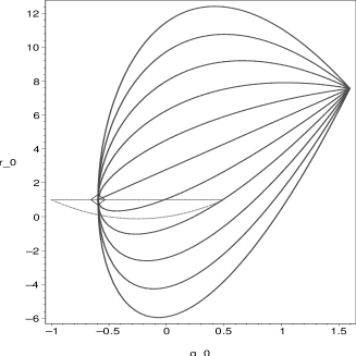
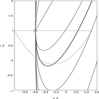
Figure 2: Present values of $q$ and $r$ for matter+quintessence with an exponential potential.
Top panel: From top to bottom the different curves have $\lambda=-5,-4,-3,-2,-1,0,1,2,3,4,5$. They all start at the point $q_{0}(\Omega_{\rm kin}=.73)=1.595$, $r_{0}(\Omega_{\rm kin}=.73)=7.57)$ [matter+Zeldovich gas ($p_{\rm x}=\rho_{\rm x}$)]. As $\Omega_{\rm kin}$ decreases when we move to the left, they join at the point $q_{0}(\Omega_{\rm kin}=0)=-0.595$, $r_{0}(\Omega_{\rm kin}=0)=1)$ ($\Lambda\rm CDM$, marked with a diamond). The dotted curve shows the area all matter+quiessence models must lie within at all times.
Bottom panel: Zoom-in of the figure above. Here the curve having $\lambda^{2}=2$ is also plotted (thick line).

As we can see from equations (45)-(46), when $\Omega_{\rm kin0}=0$, $q_{0}$ and $r_{0}$ are independent of $\lambda$, and have the same values as in the $\Lambda$CDM model. This is obvious, since taking away the kinetic term will reduce quintessence to LIVE. However, when $\Omega_{\rm kin0}$ is slightly greater then $0$ we can make $r_{0}$ as large or as small as we like, by choosing $|\lambda|$ sufficiently large. There is no reason all quintessence models should lie inside the constant-$w$-curve. However, in order to get an accelerating universe today we must have $\lambda^{2}<2$. But also for $\lambda^{2}<2$ the present values of $q_{0}$ and $r_{0}$ can lie outside the constant-$w$-curve. In fact, when we move on to the time-evolving statefinders, plotting $q$ and $r$ as functions of time for given initial conditions, we obtain plots like figure 3.

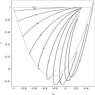
Figure 3: Time-evolution of $q$ and $r$ for models with matter and quintessence with an exponential potential. The crosses mark the present epoch. The diamond represents the present $\Lambda\rm CDM$ model. The curve on top has $\lambda=0.2$ and then $\lambda$ increases by $0.2$ for each curve going counter-clockwise until we reach $\lambda=2$ to the right. The corresponding values for $\Omega_{\rm kin}$ today are $\Omega_{\rm kin0}=0.002,0.01,0.02,0.04,0.06,0.09,0.12,0.165,0.22,0.29$. The dotted curve shows the area all matter+quiessence models must lie within at all times. We see that all models will eventually move towards this curve.

Here we have chosen as initial conditions $\Omega_{\rm m0}=0.27$ and $\Omega_{\rm k0}=0$ as above, and $h=0.71$. The last initial condition, for the quintessence field, we have chosen to be $\phi_{0}=M/100$ combined with the overall constant $A$ in the potential chosen to give $\Omega_{\rm kin0}$ as stated in the caption of figure 3. This corresponds to the universe being matter dominated at earlier times. When $\Omega_{\rm pot0}\gg\Omega_{\rm kin0}$ we have high acceleration today. Choosing $\Omega_{\rm kin0}=0$ will again give us $\Lambda$CDM. The three rightmost curves in the figure have $\lambda^{2}>2$ and no eternal acceleration, although the $\lambda=1.6$ universe accelerates today. It seems that in order to get a universe close to what we observe, $r$ and $q$ for models with matter+quintessence with an exponential potential will essentially lie within the same area as matter+quiessence models. In figure 4 we have plotted the trajectories in the $s_{0}$–$r_{0}$-plane and the $s_{0}$–$q_{0}$-plane for the same models as in figure 2, to be compared with figures 5c and 5d in Alam et al. (2003).

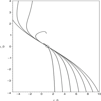
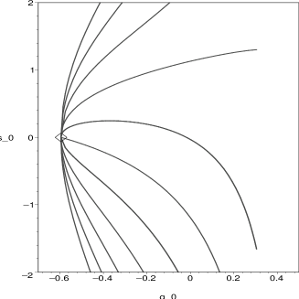
Figure 4: Present values of the statefinder parameters and the deceleration parameter for models with matter and quintessence with an exponential potential. The diamond represents the $\Lambda\rm CDM$ model.
Top panel: From left to right the different curves have $\lambda=-5,-4,-3,-2,-1,0,1,2,3,4,5$.
Bottom panel: From top to bottom the different curves have $\lambda=-5,-4,-3,-2,-1,0,1,2,3,4,5$.

Choosing instead a power-law potential $V(\phi)=A\phi^{-\alpha}$ gives $V^{\prime}=-\frac{\alpha}{\phi}V$ and

$$q = \frac{1}{2}\Omega_{\rm m}+2\Omega_{\rm kin}-\Omega_{\rm pot}$$ (47)

$$r = \Omega_{\rm m}+10\Omega_{\rm kin}+\Omega_{\rm pot}-3\alpha\frac{M}{\phi}\sqrt{6\Omega_{\rm kin}}\Omega_{\rm pot}.$$ (48)

We see that for $\phi_{0}=M$ we get the same curves in the $q_{0}$–$r_{0}$-plane when varying $\alpha$ as we got when varying $\lambda$ in the exponential potential, see figure 2. We also see that varying $\phi_{0}$ for a given value of $\alpha$ is essentially the same as varying $\alpha$. Figure 5 shows the $q_{0}$–$r_{0}$-plane for the case $\alpha=2$.

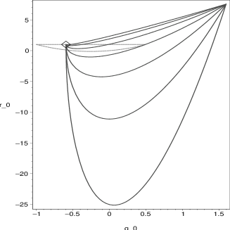
Figure 5: Present values of $q$ and $r$ for matter+quintessence with a power-law potential with $\alpha=2$. From top to bottom the different curves have $\phi_{0}=8M,4M,2M,M,\frac{M}{2},\frac{M}{4},\frac{M}{8}$.The diamond represents the $\Lambda\rm CDM$ model. The dotted curve shows the area all matter+quiessence models must lie within at all times.

Figure 6 shows an example of time-evolving statefinders ($\phi_{0}=M$, $\Omega_{\rm kin0}=0.05$, $\Omega_{\rm m0}=0.27$ $\Omega_{\rm k0}=0$, $h$=0.71). If one compares this plot with figure 1b in Alam et al. (2003), the two do not quite agree. Alam et al. (2003) do not give detailed information about the initial conditions for the quintessence field. Our initial conditions correspond to a universe which was matter-dominated up to now, when quintessence is taking over.

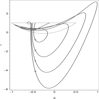
Figure 6: Time-evolution of $q$ and $r$ for models with matter and quintessence with a power-law potential. The crosses mark the present epoch, the diamond represents the present $\Lambda\rm CDM$ model. All models start out from the horizontal $\Lambda\rm CDM$ line and will eventually end up as a deSitter Universe ($q=-1,r=1$). The curve going deepest down has $\alpha=5$ and moving upwards we have $\alpha=4,3,2,1$. The dotted curve shows the area all matter+quiessence models must lie within at all times. Obviously the same is not the case for matter+quintessence models.

2.3 Dark energy fluid models

We will now find expressions for $r$ and $s$ which are valid even if the dark energy does not have an equation of state of the form $p_{\rm x}=w\rho_{\rm x}$. This is the case e.g. in the Chaplygin gas models (Kamenshchik, Moschella & Pasquier 2001; Bilic, Tupper & Viollier 2002). The expression for the deceleration parameter can be written as

$$q=\frac{1}{2}\left(1+3\frac{p_{\rm x}}{\rho_{\rm x}}\right)\Omega,$$ (49)

and using this in equation (15) we find

$$r = \left(1-\frac{3}{2}\frac{\dot{p}_{\rm x}}{H\rho_{\rm x}}\right)\Omega$$ (50)

$$s = -\frac{1}{3H}\frac{\dot{p}_{\rm x}}{p_{\rm x}}.$$ (51)

If the universe contains only dark energy with an equation of state $p=p(\rho)$, then

$$\dot{p}=\dot{\rho}\frac{\partial p}{\partial\rho}=-3H(\rho+p)\frac{\partial p}{\partial\rho},$$ (52)

which leads to

$$r = \left[1+\frac{9}{2}\left(1+\frac{p}{\rho}\right)\frac{\partial p}{\partial\rho}\right]\Omega$$ (53)

$$s = \left(1+\frac{\rho}{p}\right)\frac{\partial p}{\partial\rho}.$$ (54)

If the universe contains cold matter and dark energy these expressions are generalized to

$$r = \left(1+\frac{9}{2}\frac{\rho_{\rm x}+p_{\rm x}}{\rho_{\rm m}+\rho_{\rm x}}\frac{\partial p_{\rm x}}{\partial\rho_{\rm x}}\right)\Omega$$ (55)

$$s = \left(1+\frac{\rho_{\rm x}}{p_{\rm x}}\right)\frac{\partial p_{\rm x}}{\partial\rho_{\rm x}}.$$ (56)

The Generalized Chaplygin Gas (GCG) has an equation of state (Bento, Bertolami & Sen 2002)

$$p=-\frac{A}{\rho^{\alpha}},$$ (57)

and integration of the energy conservation equation gives

$$\rho=\left[A+Ba^{-3(1+\alpha)}\right]^{\frac{1}{1+\alpha}},$$ (58)

where $B$ is a constant of integration. This can be rewritten as

$$\rho=\rho_{0}\left[A_{\rm s}+(1-A_{\rm s})x^{3(1+\alpha)}\right]^{\frac{1}{1+\alpha}},$$ (59)

where $\rho_{0}=(A+B)^{1/(1+\alpha)}$, and $A_{\rm s}=A/(A+B)$. For a flat universe with matter and a GCG, the Hubble parameter is given by

$$\frac{H^{2}(x)}{H_{0}}=\Omega_{\rm m0}x^{3}+(1-\Omega_{\rm m0})\left[A_{\rm s}+(1-A_{\rm s})x^{3(1+\alpha)}\right]^{\frac{1}{1+\alpha}}.$$ (60)

This leads to the following expressions for $q(x)$ and $r(x)$:

$$q(x) = \frac{3}{2}\frac{\Omega_{\rm m0}x^{3}+(1-\Omega_{\rm m0})(1-A_{\rm s})\ v^{\frac{3}{\beta}-1}\ x^{\beta}}{\Omega_{\rm m0}x^{3}+(1-\Omega_{m0})\ v^{3/{\beta}}}-1$$ (61)

$$r(x) = 1-3\ \frac{x}{h^{2}(x)}f(x)+\frac{3}{2}\ \frac{x^{2}}{h^{2}(x)}f^{\prime}(x),$$ (62)

where $\beta=3(1+\alpha)$, $h(x)=H(x)/H_{0}$, and

$$v = A_{\rm s}+(1-A_{\rm s})x^{\beta}$$ (63)

$$f(x) = \Omega_{\rm m0}x^{2}+(1-\Omega_{\rm m0})(1-A_{\rm s})v^{\frac{3}{\beta}-1}\ x^{\beta-1}.$$ (64)

In the $r$-$s$ plane, the GCG models will lie on curves given by (see Gorini, Kamenshchik & Moschella 2003)

$$r=1-\frac{9}{2}\frac{s(s+1)}{\alpha}.$$ (65)

We note that a recent comparison of GCG models with SNIa data found evidence for $\alpha>1$ (Bertolami et al. 2004).

2.4 Cardassian models

As an alternative to adding a negative-pressure component to the energy-momentum tensor of the Universe, one can take the view that the present phase of accelerated expansion is caused by gravity being modified, e.g. by the presence of large extra dimensions. For a general discussion of extra-dimensional models and statefinder parameters, see Alam & Sahni (2002).

As an example, we will consider the Modified Polytropic Cardassian ansatz (MPC) (Freese & Lewis 2002; Gondolo & Freese 2003), where the Hubble parameter is given by

$$H(x)=H_{0}\sqrt{\Omega_{\rm m0}x^{3}\Bigl{(}1+u\Bigr{)}^{1/\psi}},$$ (66)

with

$$u=u(x)=\frac{\Omega_{\rm m0}^{-\psi}\ -\ 1}{x^{3(1-n)\psi}},$$ (67)

and where $n$ and $\psi$ are new parameters ($\psi$ is usually called $q$ in the literature, but we use a different notation here to avoid confusion with the deceleration parameter). For this model, the deceleration parameter is given by

$$q(x)=\frac{3}{2}\Biggl{[}\frac{1+nu}{1+u}\Biggr{]}-1$$ (68)

and the statefinder $r$ by

$$r(x) = 1-\frac{9}{4}\ \frac{1+nu}{1+u}\Biggl{[}1+\frac{u(1-n)-(1+nu)}{1+u}$$ (69)

$$- 2q\frac{(1-n)^{2}u}{(1+u)(1+nu)}.\Biggr{]}$$

2.5 The luminosity distance to third order in $z$

The statefinder parameters appear when one expands the luminosity distance to third order in the redshift $z$. Although this expansion has been presented earlier (Chiba & Nakamura 1998; Visser 2003) in a slightly different notation, we carry out this derivation here for completeness. The luminosity distance is given by the expression

$$d_{\rm L}=\frac{1+z}{H_{0}\sqrt{|\Omega_{\rm k0}}}{\cal S}_{k}(\sqrt{|\Omega_{\rm k0}|}I),$$ (70)

where ${\cal S}_{\rm k}(x)=\sin x$ for $k=1$, ${\cal S}_{\rm k}(x)=x$ for $k=0$, ${\cal S}_{\rm k}(x)=\sinh x$ for $k=-1$, and

$$I=H_{0}\int_{0}^{z}\frac{dz}{H(z)}.$$ (71)

Using the approximation

$${\cal S}_{\rm k}(x)\approx x-\frac{k}{6}x^{3},$$ (72)

one finds to third order in $z$

$$H_{0}d_{\rm L}\approx(1+z)I\left(1+\frac{1}{6}\Omega_{\rm k0}I^{2}\right).$$ (73)

Taylor expanding the Hubble parameter to second order in $z$, we have

$$I\approx\int_{0}^{z}\frac{dz}{1+\gamma z+\kappa z^{2}},$$ (74)

with

$$\gamma = \frac{1}{H_{0}}\left(\frac{dH}{dz}\right)_{z=0},$$ (75)

$$\kappa = \frac{1}{2H_{0}}\left(\frac{d^{2}H_{0}}{dz^{2}}\right)_{z=0}.$$ (76)

By using $(1+y)^{-1}\approx 1-y+y^{2}$ with $y=\gamma z+\kappa z^{2}$, we get to third order in $z$

$$(1+z)I \approx (1+z)\int_{0}^{z}\left[1-\gamma z+(\gamma^{2}-\kappa)z^{2}\right]dz$$ (77)

$$= z+\left(1-\frac{1}{2}\gamma\right)z^{2}$$

$$- \left(\frac{1}{2}\gamma+\frac{1}{3}\kappa-\frac{1}{3}\gamma^{2}\right)z^{3}.$$

We wish to express $\gamma$ and $\kappa$ in terms of the deceleration parameter

$$q_{0}=-\left(\frac{\ddot{a}a}{\dot{a}^{2}}\right)_{t=t_{0}},$$ (78)

and the statefinder

$$r_{0}=\left(\frac{a^{2}\stackrel{{\scriptstyle{\bf\ldots}}}{{a}}}{\dot{a}^{3}}\right)_{t=t_{0}}.$$ (79)

From $H=\dot{a}/a$ one finds

$$\dot{H} = -(1+q)H^{2},$$ (80)

$$\ddot{H} = (r+3q+2)H^{3}.$$ (81)

From $a=(1+z)^{-1}$, one gets $H=-\dot{z}/(1+z)$, and hence

$$\frac{d}{dz} = -\frac{1}{(1+z)H}\frac{d}{dt},$$ (82)

$$\frac{d^{2}}{dz^{2}} = \frac{1}{(1+z)H}\frac{d}{dt}\left[\frac{1}{(1+z)H}\frac{d}{dt}\right].$$ (83)

After some algebra one then finds

$$\gamma = 1+q_{0},$$ (84)

$$\kappa = \frac{1}{2}(r_{0}-q_{0}^{2}).$$ (85)

Substitution of these expressions for $\gamma$ and $\kappa$ in (77) gives

$$(1+z)I \approx z\Biggl{[}1+\frac{1}{2}(1-q_{0})z-\frac{1}{6}(1+r_{0}$$ (86)

$$- q_{0}-3q_{0}^{2})z^{2}\Biggr{]},$$

and equation (73) then finally leads to

$$d_{\rm L} \approx \frac{z}{H_{0}}\Biggl{[}1+\frac{1}{2}(1-q_{0})z-\frac{1}{6}(1+r_{0}-q_{0}$$ (87)

$$- 3q_{0}^{2}-\Omega_{\rm k0})z^{2}\Biggr{]}.$$

One can also find an expression for the present value of the time derivative of the equation of state parameter $w$ in terms of the statefinder $r_{0}$. A Taylor expansion to first order in $z$ gives

$$w(z)=w_{0}-\frac{\dot{w}(t_{0})}{H_{0}}z,$$ (88)

From equation (14) we have

$$w_{0}=\frac{2q_{0}-\Omega_{\rm m0}-\Omega_{\rm x0}}{3\Omega_{\rm x0}},$$ (89)

and from equation (24) we get

$$\dot{w}(t_{0})=\frac{2}{3}\frac{H_{0}}{\Omega_{\rm x0}}\left\{\Omega_{\rm m0}+\left[1+\frac{9}{2}w_{0}(1+w_{0})\right]\Omega_{\rm x0}-r_{0}\right\}.$$ (90)

Hence

$$w(z)\approx w_{0}-\frac{2}{3}\left[1+\frac{9}{2}w_{0}(1+w_{0})+\frac{\Omega_{\rm m0}-r_{0}}{\Omega_{\rm x0}}\right]z.$$ (91)

3 Lessons drawn from current SNIa data

In this section we will consider the SNIa data presently available, in particular whether one can use them to learn about the statefinder parameters. We will use the recent collection of SNIa data in Riess et al. (2004), their ‘gold’ sample consisting of 157 supernovae at redshifts between $\sim 0.01$ and $\sim 1.7$.

3.1 Model-independent constraints

The approximation to $d_{\rm L}$ in equation (87) is independent of cosmological model, the only assumption made is that the Universe is described by the Friedmann-Robertson-Walker metric. We see that, in addition to $H_{0}$, this third-order expansion of $d_{\rm L}$ depends on $q_{0}$ and the combination $r_{0}-\Omega_{\rm k0}$. Fitting these parameters to the data, we find the constraints shown in Fig. 7. The results are consistent with those of similar analyses in Caldwell & Kamionkowski (2004) and Gong (2004).

Figure 7: Likelihood contours (68, 95 and 99%) resulting from a fit of the expansion of the luminosity distance to third order in $z$.

Figure 8: Marginalized probability distributions for $q_{0}$ (full line) and $r_{0}-\Omega_{\rm k0}$ (dotted line).

In figure 8 we show the marginalized distributions for $q_{0}$ and $r_{0}-\Omega_{\rm k0}$. We note that the supernova data firmly support an accelerating universe, $q_{0}<0$ at more than 99% confidence. However, about the statefinder parameter $r_{0}$, little can be learned without an external constraint on the curvature. Imposing a flat universe, e.g. by inflationary prejudice or by invoking the CMB peak positions, there is still a wide range of allowed values for $r_{0}$. This is an indication of the limited ability of the current SNIa data to place constraints on models of dark energy. There is only limited information on anything beyond the present value of the second derivative of the Hubble parameter.

Under the assumption of a spatially flat universe, $\Omega_{\rm k0}=0$, with $\Omega_{\rm m0}=0.3$, one can use equations (89) and (91) to obtain constraints on $w_{0}$ and $w_{1}$ in the expansion $w(z)=w_{0}+w_{1}z$ of the equation of state of dark energy. The resulting likelihood contours are shown in figure 9. As can be seen in this figure, there is no evidence for time evolution in the equation of state, the observations are consistent with $w_{1}=0$. The present supernova data show a slight preference for a dark energy component of the ‘phantom’ type with $w_{0}<-1$ (Caldwell 2002). Note, however, that the relatively tight contours obtained here are caused by the strong prior $\Omega_{\rm m0}=0.3$. It should also be noted that the third-order expansion of $d_{\rm L}$ is not a good approximation to the exact expression for high $z$ and in some regions of the parameter space.

Figure 9: Likelihood contours (68, 95 and 99%) for the coefficients $w_{0}$ and $w_{1}$ in the linear approximation to the equation of state $w(z)$ of dark energy, resulting from a fit of the expansion of the luminosity distance to third order in $z$.

3.2 Direct test of models against data

The standard way of testing dark energy models against data is by maximum likelihood fitting of their parameters. In this subsection we will consider the following models:

1. The expansion of $d_{\rm L}$ to second order in $z$, with $h$ and $q_{0}$ as parameters.

2. The third-order expansion of $d_{\rm L}$, with $h$, $q_{0}$, and $r_{0}-\Omega_{\rm k0}$ as parameters.

3. Flat $\Lambda{\rm CDM}$ models, with $\Omega_{\rm m0}$ and $h$ as parameters to be varied in the fit.

4. $\Lambda{\rm CDM}$ with curvature, so that $\Omega_{\rm m0}$, $\Omega_{\Lambda 0}$ (the contribution of the cosmological constant to the energy density in units of the critical density, evaluated at the present epoch), and $h$ are varied in the fits.

5. Flat quiessence models, that is, models with a constant equation of state $w$ for the dark energy component. The parameters to be varied in the fit are $\Omega_{\rm m0}$, $w$, and $h$.

6. The Modified Polytropic Cardassian (MPC) ansatz, with $\Omega_{\rm m0}$, $q$, $n$, and $h$ as parameters to be varied.

7. The Generalized Chaplygin Gas (GCG), with $\Omega_{\rm m0}$, $A_{\rm s}$, $\alpha$, and $h$ as parameters to be varied.

8. The ansatz of Alam et al. (2003),

   $$H=H_{0}\sqrt{\Omega_{\rm m0}x^{3}+A_{0}+A_{1}x+A_{2}x^{2}},$$ (92)

   where we restrict ourselves to flat models, so that $A_{0}=1-\Omega_{\rm m0}-A_{1}-A_{2}$. The parameters to be varied are $\Omega_{\rm m0}$, $A_{1}$, $A_{2}$, and $h$.

Note that these models have different numbers of free parameters. To get an idea of which of these models is actually preferred by the data, we therefore employ the Bayesian Information Criterion (BIC) (Schwarz 1978; Liddle 2004). This is an approximation to the Bayes factor (Jeffreys 1961), which gives the posterior probability of one model relative to another assuming that there is no objective reason to prefer one of the models prior to fitting the data. It is given by

$${\cal B}=\chi^{2}_{\rm min}+N_{\rm par}\ln N_{\rm data},$$ (93)

where $\chi^{2}_{\rm min}$ is the minimum value of the $\chi^{2}$ for the given model against the data, $N_{\rm par}$ is the number of free parameters, and $N_{\rm data}$ is the number of data points used in the fit. As a result of the approximations made in deriving it, ${{\cal B}}$ is given in terms of the minimum $\chi^{2}$, even though it is related to the integrated likelihood. The preferred model is the one which minimizes ${\cal B}$. In table 1 we have collected the results for the best-fitting models.

Table 1: Results of fitting the models considered in this subsection to the SNIa data

Model	$\chi^{2}_{\rm min}$	# parameters	${{\cal B}}$
2. order expansion	177.1	2	187.2
3. order expansion	162.3	3	177.5
Flat $\Lambda{\rm CDM}$	163.8	2	173.9
$\Lambda{\rm CDM}$ with curvature	161.2	3	176.4
flat + constant EoS	160.0	3	175.2
MPC	160.3	4	180.5
GCG	161.4	4	181.6
Alam et al.	160.5	4	180.7

When comparing models using the BIC, the rule of thumb is that a difference of 2 in the BIC is positive evidence against the model with the larger value, whereas if the difference is 6 or more, the evidence against the model with the larger BIC is considered strong. The second-order expansion of $d_{\rm L}$ is then clearly disfavoured, thus the current supernova data give information, although limited, on $r_{0}-\Omega_{\rm k0}$. We see that there is no indication in the data that curvature should be added to the $\Lambda{\rm CDM}$ model. Also, the last three models in table 1 seem to be disfavoured. One can conclude that there is no evidence in the current data that anything beyond flat $\Lambda{\rm CDM}$ is required. This does not, of course, rule out any of the models, but tells us that the current data are not good enough to reveal physics beyond spatially flat $\Lambda{\rm CDM}$. A similar conclusion was reached by Liddle (2004) using a more extensive collection of cosmological data sets and considering adding parameters to the flat $\Lambda{\rm CDM}$ model with scale-invariant adiabatic fluctuations.

3.3 Statefinder parameters from current data

If the luminosity distance $d_{\rm L}$ is found as a function of redshift from observations of standard candles, one can obtain the Hubble parameter formally from

$$H(x)=\left[\frac{d}{dx}\left(\frac{d_{\rm L}}{x}\right)\right]^{-1}.$$ (94)

However, since observations always contain noise, this relation cannot be applied straightforwardly to the data. Alam et al. (2003) suggested parametrizing the dark energy density as a second-order polynomial in $x$, $\rho_{\rm x}=\rho_{\rm c0}(A_{0}+A_{1}x+A_{2}x^{2})$, leading to a Hubble parameter of the form

$$H(x)=H_{0}\sqrt{\Omega_{\rm m0}x^{3}+A_{0}+A_{1}x+A_{2}x^{2}},$$ (95)

and fitting $A_{0}$, $A_{1}$, and $A_{2}$ to data. This parametrization reproduces exactly the cases $w=-1$ ($A_{1}=A_{2}=0$), $w=-2/3$ ($A_{0}=A_{2}=0$), and $w=-1/3$ ($A_{0}=A_{1}=0$), and the luminosity distance-redshift relationship is given by

$$d_{\rm L}=\frac{1+z}{H_{0}}\int_{1}^{1+z}\frac{dx}{\sqrt{\Omega_{\rm m0}x^{3}+A_{0}+A_{1}x+A_{2}x^{2}}}.$$ (96)

Having fitted the parameters $A_{0}$, $A_{1}$, and $A_{2}$ to e.g. supernova data using (96), one can then find $q$ and $r$ by substituting equation (95) into (5) and (6):

$$q(x) = \frac{1}{2}\left(1-\frac{A_{2}x^{2}+2A_{1}x+3A_{0}}{\Omega_{\rm m0}x^{3}+A_{2}x^{2}+A_{1}x+A_{0}}\right)$$ (97)

$$r(x) = \frac{\Omega_{\rm m0}x^{3}+A_{0}}{\Omega_{\rm m0}x^{3}+A_{0}+A_{1}x+A_{2}x^{2}},$$ (98)

and furthermore the statefinder $s$ is found to be

$$s(x)=\frac{2}{3}\frac{A_{1}x+A_{2}x^{2}}{3A_{0}+2A_{1}x+A_{2}x^{2}},$$ (99)

and the equation of state is given by

$$w(x)=-1+\frac{1}{3}\frac{A_{1}x+2A_{2}x^{2}}{A_{0}+A_{1}x+A_{2}x^{2}}.$$ (100)

The simulations of Alam et al. (2003) indicated that the statefinder parameters can be reconstructed well from simulated data based on a range of dark energy models, so we will for now proceed on the assumption that the parametrization in equation (95) is adequate for the purposes of extracting $q$, $r$ and $s$ from SNIa data. We comment this issue in section 4.

In figure 10 we show the deceleration parameter $q$ and the statefinder $r$ extracted from the current SNIa data. The error bars in the figure are $1\sigma$ limits. We have also plotted the model predictions for the same quantities (based on best-fitting parameters with errors) for $\Lambda{\rm CDM}$, quiessence, and the MPC. The figure shows that all models are consistent at the $1\sigma$ level with $q$ and $r$ extracted using equation (95). Thus, with the present quality of SNIa data, the statefinder parameters are, not surprisingly, no better at distinguishing between the models than a direct comparison with the SNIa data.

Figure 10: The deceleration parameter $q$ and the statefinder $r$ extracted from current SNIa data using the Alam parametrization of $H$ (top row), for $\Lambda{\rm CDM}$ (second row), quiessence (third row), and the Modified Polytropic Cardassian ansatz (bottom row)

We next look at simulated data to get an idea of how the situation will improve with future data sets.

4 Future data sets

We will now make an investigation of what an idealized SNIa survey can teach us about statefinder parameters and dark energy, following the procedure in Saini, Weller & Bridle (2004).

A SNAP-like satellite is expected to observe $\sim$2000 SN up to $z\sim 1.7$. Dividing the interval $0<x\leq 1.7$ into 50 bins, we therefore expect $\sim$40 observations of SN in each bin. Empirically, SNIa are very good standard candles with a small dispersion in apparent magnitude $\sigma_{\rm mag}=0.15$, and there is no indication of redshift evolution. The apparent magnitude is related to the luminosity distance through

$$m(z)={{\cal M}}+5\log D_{\rm L}(z),$$ (101)

where ${{\cal M}}=M_{0}+5\log[H_{0}^{-1}{\rm Mpc}^{-1}]+25$. The quantity $M_{0}$ is the absolute magnitude of type Ia supernovae, and $D_{\rm L}(z)=H_{0}d_{\rm L}(z)$ is the Hubble constant free luminosity distance. The combination of absolute magnitude and the Hubble constant, ${{\cal M}}$, can be calibrated by low-redshift supernovae (Hamuy et al. 1993; Perlmutter et al. 1999). The dispersion in the magnitude, $\sigma_{\rm mag}$, is related to the uncertainty in the distance, $\sigma$, by

$$\frac{\sigma}{d_{\rm L}(z)}=\frac{\ln 10}{5}\sigma_{\rm mag},$$ (102)

and for $\sigma_{\rm mag}=0.15$, the relative error in the luminosity distance is $\sim 7$%. If we assume that the $d_{L}$ we calculate for each $z$ value is the mean of all $d_{L}$s in that particular bin, the errors reduce from 7% to $0.07/\sqrt{40}\approx 0.01=1\%$. We do not add noise to the simulated $d_{\rm L}$, and hence our results give the ensemble average of the parameters we fit to the simulated data sets.

4.1 A $\Lambda{\rm CDM}$ universe

We first simulate data based on a flat $\Lambda{\rm CDM}$ model with $\Omega_{\rm m0}=0.3$, $h=0.7$, giving the data points shown in figure 11.

Figure 11: Binned, simulated data set for a flat $\Lambda{\rm CDM}$ universe with $\Omega_{\rm m0}=0.3$. The $1\sigma$ error bars are also shown.

To this data set we first fit the quiessence model, the MPC, the GCG, and the parametrization of $H$ from equation (95). Since all models reduce to $\Lambda{\rm CDM}$ for an appropriate choice of parameters, distinguishing between them based on the $\chi^{2}$ per degree of freedom alone is hard. Based on the best-fitting values and error bars on the parameters $A_{0}$, $A_{1}$, and $A_{2}$ in equation (95) we can reconstruct the statefinder parameters from eqs. (97) – (99). In figure 12 we show the deceleration parameter and statefinder parameters reconstructed from the simulated data.

Figure 12: The statefinder parameters and the deceleration parameter for the best-fitting reconstruction of the simulated data based on $\Lambda{\rm CDM}$, using the parametrization of Alam et al. The $1\sigma$ error bars are also shown.

The statefinders can be reconstructed quite well in this case, e.g. we see clearly that $r$ is equal to one, as it should for flat $\Lambda{\rm CDM}$.

Figure 13: The statefinder parameters for a selection of models, evaluated at the best-fitting values of their respective parameters to the simulated $\Lambda{\rm CDM}$ dataset, with errors included.

In figure 13 we show the statefinders for a selection of models, obtained by fitting their respective parameters to the data, and using the expressions for $q$ and $r$ for the respective models derived in earlier sections, e.g. equation (61) and (62) for the Chaplygin gas. Since all models reduce to $\Lambda{\rm CDM}$ for the best-fitting parameters, their $q$ and $r$ values are also consistent with $\Lambda{\rm CDM}$. Thus, if the dark energy really is LIVE, a SNAP-type experiment should be able to demonstrate this.

4.2 A Chaplygin gas universe

We have also carried out the same reconstruction exercise using simulated data based on the GCG with $A_{\rm s}=0.4$, $\alpha=0.7$, see figure 14.

Figure 14: Simulated luminosity distance-redshift relationship for the Generalized Chaplygin Gas with $A_{\rm s}=0.4$, $\alpha=0.7$.

Figure 15: The statefinder parameters and the deceleration parameter for the best-fitting reconstruction of the simulated data based on the GCG, using the parametrization of Alam et al. The $1\sigma$ error bars are also shown.

Figure 15 shows $q$ and $r$ reconstructed using the parametrization of $H$. The same quantities for the models considered, based on their best-fitting parameters to the simulated data, are shown in figure 16.

Figure 16: The statefinder parameters for a selection of models, evaluated at the best-fitting values of their respective parameters to the simulated Chaplygin gas data set, with errors included.

For the Cardassian model, the best-fitting value for the parameter $n$, $n_{\rm bf}$, depends on the extent of the region over which we allow $n$ to vary. Extending this region to larger negative values for $n$ moves $n_{\rm bf}$ in the same direction. However, the minimum $\chi^{2}$ value does not change significantly. This is understandable, since $H(x)$ for the MPC model is insensitive to $n$ for large, negative values of $n$. The quantities $r(x)$ and $q(x)$ also depend only weakly on the allowed range for $n$, whereas their error bars are sensitive to this parameter. We chose to impose a prior $n>-1$, producing the results shown in figure 16. The best-fitting values for $\psi$ and $n$ were, respectively, $0.06$ and $-0.94$.

Figure 17 shows the deceleration parameter extracted from the Alam et al. parametrization (full line), with $1\sigma$ error bars. Also plotted is the best fit $q(z)$ from the quiessence (squares), Cardassian (triangles) and Chaplygin (asterisk) models. We note that the $q(z)$ from the Alam et al. parametrization has a somewhat deviating behaviour from the input model, especially at larger $z$. Also, no model can be excluded on the basis of their predictions for $q(z)$

Figure 18 shows the same situation for the statefinder parameter $r(z)$. Note again that for large $z$, the recovered statefinder from the Alam et al. parametrization does not correspond well with the input model. As with the case for $q(z)$, the quiessence and Cardassian models follow each other closely. These, however, do not agree with the input model for low values of $z$ (similar to the case for $q(z)$ they diverge for low $z$). Comparing the statefinder $r$ for the quiessence and Cardassian models with that of the input GCG model, indicates that, not surprisingly, neither of them is a good fit to the data.

Figure 17: Comparison of $q(z)$ extracted using the parametrized $H(z)$ with $q(z)$ for the various best-fitting models. Error bars are only shown on the values extracted using the Alam et al. parametrization, but in the other cases they are roughly of the same size as the symbols.

Figure 18: Comparison of $r(z)$ extracted using the parametrized $H(z)$ with $r(z)$ for the various best-fitting models. Error bars are only shown on the values extracted using the Alam et al. parametrization, but in the other cases they are roughly of the same size as the symbolsS.

This exercise indicates that the statefinders can potentially distinguish between dark energy models, if $q$, $r$ and $s$ can be extracted from the data in a reliable, model-independent way. However, the fact that $r$ extracted from the simulated data using the Alam et al. parametrization does not agree well with the true $r$ of the underlying model for $z>0.5$, indicates that one needs a better parametrization in order to use statefinder parameters as empirical discriminators between dark energy models.

5 Conclusions

We have investigated the statefinder parameters as a means of comparing dark energy models. As a theoretical tool, they are very useful for visualizing the behaviour of different dark energy models. Provided they can be extracted from the data in a reliable, model-independent way, they can give a first insight into the type of model which is likely to describe the data. However, SNIa data of quality far superior to those presently available are needed in order to distinguish between the different models. And even with SNAP-quality data, there may be difficulties in distinguishing between models based on the statefinder parameters alone. Furthermore, the parametrization of $H(z)$ used here and in Alam et al. (2003) is probably not optimal, as shown in section 4.2. The same conclusion was reached in a recent investigation by Jönsson et al. (2004), where they considered reconstruction of the equation of state $w(x)$ from SNIa data using equation (100). They found that this parametrization forces the behaviour of $w(x)$ onto a specific set of tracks, and may thus give spurious evidence for redshift evolution of the equation of state. Although this conclusion has been contested by Alam et al. (2004), it is clear that finding a parametrization which is sufficiently general, and at the same time with reasonably few parameters is an important task for future work.