The HIPASS catalogue – I. Data presentation

Abstract

The Hi Parkes All-Sky Survey (Hipass) Catalogue forms the largest uniform catalogue of Hi sources compiled to date, with 4,315 sources identified purely by their Hi content. The catalogue data comprise the southern region $\delta<+2\degr$ of Hipass, the first blind Hi survey to cover the entire southern sky. RMS noise for this survey is 13 mJy beam^-1 and the velocity range is $-$1,280 to 12,700 km s^-1. Data search, verification and parametrization methods are discussed along with a description of measured quantities. Full catalogue data are made available to the astronomical community including positions, velocities, velocity widths, integrated fluxes and peak flux densities. Also available are on-sky moment maps, position-velocity moment maps and spectra of catalogue sources. A number of local large-scale features are observed in the space distribution of sources including the Super-Galactic plane and the Local Void. Notably, large-scale structure is seen at low Galactic latitudes, a region normally obscured at optical wavelengths.

Table 1: Parameters of existing blind Hi surveys. $\delta v$ is the velocity resolution. $N^{lim}_{HI}$ is the limiting Hi column density for gas filling the beam. Column density limits are $5\sigma$ and calculated with $\Delta V=100$km s^-1, scaling RMS appropriately according to the velocity resolution. SCC, BGC and Hicat all use Hipass data. The SCC sample searches $\delta<-62\degr$ and the BGC searches $\delta<0\degr$ and $S_{p}>$ 116 mJy. The references cited are as follows: ¹Shostak (1977), ²Krumm & Brosch (1984),³Kerr & Henning (1987), Henning (1992), ⁴Sorar (1994),Zwaan et al. (1997),Spitzak & Schneider (1998), ⁶Rosenberg & Schneider (2000), ⁷Henning et al. (2000), ⁸Kilborn et al. (2002), Braun, Thilker & Walterbos (2003), ¹⁰Lang et al. (2003), ¹¹Koribalski et al. (2004), ¹² this paper.

Name	Area	Beam Size	Velocity	$\delta v$	RMS	$N^{lim}_{HI}$	Telescope	Sources
	(deg2)	(arcmin)	(km s-1)	(km s-1)	(mJy beam-1)	(cm-2)
Shostak1	85,
70,
11	10.8	$\sim$$-$800 to $\sim$2,835	11	32,
44,
18	1.6$\times 10^{19}$, 2.3$\times 10^{19}$, 9.2$\times 10^{18}$	91m Green Bank	1a
Krumm &
Brosch2	$\sim$35,
$\sim$44	10.8	6,300 to 9,600,
5,300 to 8,500	$\sim$45	22	2.2$\times 10^{19}$	91m Green Bank	0
Henning3	7,204 pointings	10.8	$-$400 to 7,500	22	-	-	91m Green Bank	37
AHISS4	65	3.3	$<$7,400	16	0.75	4.3$\times 10^{18}$	305m Arecibo	66
Slice Survey5	55	3.3	100 to 8,340	16	1.7	9.6$\times 10^{18}$	305m Arecibo	75
ADBS6	430	3.3	$<$7,980	34	3.5	2.8$\times 10^{19}$	305m Arecibo	265
HIZSS7	1,840	15.5	$-$1,200 to 12,700	27	15	5.0$\times 10^{18}$	64m Parkes	110
SCC8§	$\sim 2400$	15.5	$-$1,280 to 12,700	18	13	4.0$\times 10^{18}$	64m Parkes	536
WRST Wide Field Survey9	1,800	49	$-$1,000 to 6,500	17	18	4.8$\times 10^{17}$	Westerbork Array	155
HIJASS10b	1,115	12	$-$3,500 to 10,000	18	16	7.3$\times 10^{18}$	76m Jodrell Bank	222
BGC11§	20,626	15.5	$-$1,200 to 8,000	18	13	1.7$\times 10^{19}$d	64m Parkes	1,000
Hicat 12§	21,346	15.5	300 to 12,700	18c	13	4.0$\times 10^{18}$	64m Parkes	4,315
aNot certainly extragalactic.
bSurvey in progress.
cData velocity resolution. Parametrization was carried out with additional Hanning smoothing, giving a velocity resolution of 26.4 km s-1.
dBased on catalogue selection limits rather than 5$\sigma$ survey limit.

1 Introduction

The neutral hydrogen (Hi) content of galaxies provides a unique and fundamental perspective into the nature and evolution of galaxies, being intimately linked to both the dark matter component of galaxies along with their ability to form stars.

Surveys for Hi in galaxies, however, are limited by the relative weakness of Hi photons. Despite a cosmological mass density ratio of Hi to luminous matter of only 1:10, the improbability of the Hi hyperfine transition and weakness of photons emitted mean that the received power ratio favours optical photons by many orders of magnitude. In combination with observational limitations, this has traditionally necessitated either blind surveys of relatively small volumes (eg. Shostak 1977, Krumm & Brosch 1984, Kerr & Henning 1987, Henning 1992, Sorar 1994, Zwaan et al. 1997, Spitzak & Schneider 1998, Rosenberg & Schneider 2000), or targeted surveys across larger regions through the use of existing, typically optical, catalogues (eg. Fisher & Tully 1981, Mathewson et al. 1992, Giovanelli et al. 1997, Haynes et al. 1999). Parameters for existing blind Hi surveys are summarized in Table The HIPASS catalogue – I. Data presentation.

With the advent of Multibeam receivers on the Parkes and Jodrell Bank radio telescopes, along with the forthcoming ALFA instrument at Arecibo, large untargeted surveys are now practicable for the first time. In this work we discuss results from the Hi Parkes All-Sky Survey (Hipass), a blind survey of the entire sky $\delta<+25\degr$. Various extragalactic catalogue subsets from this survey have already been completed including: Kilborn et al. (2002, $\delta<-62$); Koribalski et al. (2004, $\delta<0\degr$ and $S_{\rm p}>116$ mJy) and companion analysis papers Zwaan et al. (2003, Hi mass function) and Ryan-Weber et al. (2002, newly catalogued galaxies); Waugh et al. (2002, Fornax region); and Banks et al. (1999, Centaurus A group). Presented here are results from the southern region of the survey ($\delta<+2\degr$); these data were searched for extragalactic sources to full survey depth.

A complete database of Hi-selected galaxies is important for a number of important astrophysical studies. Amongst these is a measurement of the Hi cosmic mass density, $\Omega_{\rm HI}$. At higher redshifts, $\Omega_{\rm HI}$ can be measured through damped Ly$\alpha$ systems, however at $z$=0, the only way to accurately measure $\Omega_{\rm HI}$ is through large-scale surveys for Hi emission. Galaxies under-represented in optical surveys such as low surface brightness galaxies, those with elusive optical counterparts and Malin 1 type systems (Bothun et al., 1987) are also best detected via blind Hi surveys. Gaining an accurate census of such objects is important for constraining models of galaxy formation, although not contributing a significant fraction of the overall gas mass density (Zwaan et al., 2003).

Other important applications for a large uniform catalogue of Hi sources include the measurement of large-scale structure, 2-point correlation functions, the Tully-Fisher relation, the role of hydrogen gas in the evolution of galaxy groups and the study of environments around Hi-rich galaxies compared to those of optically-selected galaxies.

In Section 2 we discuss the observational methods, data processing and basic properties of Hipass. Methods used to compile the source database are described in detail in Section 3, including the identification, verification and parametrization of sources, confused- and extended-source processing, the effects of radio-frequency interference (RFI) and recombination lines, and follow-up observations. Access to catalogue data is described in Section 4. Finally, basic property distributions are presented in Section 5 and the large-scale distribution of galaxies in Section 6. Reliability, completeness and accuracy of catalogue parameters are discussed in the companion paper by Zwaan et al. (2004, Paper II). The identification of optical counterparts to Hipass Catalogue galaxies is made in Drinkwater et al. (2004, Paper III).

2 The HI Parkes All-Sky Survey

Hipass was completed at the Parkes 64m radio telescope using the Multibeam receiver, an hexagonal array of 13 circular feed-horns installed at the focal plane of the telescope. Observations and data reduction for this survey are described in detail in Barnes et al. (2001) and Staveley-Smith et al. (1996). A brief summary is provided below.

2.1 Observations

Hipass observations were carried out from February 1997 to March 2000 for the southern portion of the survey ($\delta<+2\degr$) and to December 2001 for the northern extension ($\delta<+25\degr$). For these observations, the telescope was scanned across the sky in $8^{\circ}$ strips at a rate of $1^{\circ}$ per minute, with scans separated by 7 arcmin in RA, giving a total effective integration time of 450s beam^-1. To obtain spectra, the Multibeam correlator was used with a 64 MHz bandwidth and 1024 channel configuration, giving a velocity range of $-$1,280 to 12,700 km s^-1and a channel separation of 13.2 km s^-1  at $z=0$. Parameters for the survey are summarized in Table 2.

2.2 Data Processing

Table 2: Hipass parameters

Sky Coverage	$\delta<+25\degr$⋆
Integration time per beam	450s
Average FWHM	14.3 arcmin
Gridded FWHM	15.5 arcmin
Pixel size	4 arcmin
Velocity Range	$-$1,280 to 12,700 km s-1
Channel separation†	13.2 km s-1
Velocity Resolution	18.0 km s-1
Positional accuracy‡	1.5 arcmin
RMS noise	13 mJy beam-1
⋆ The Hipass Catalogue covers southern regions $\delta<+2\degr$
† at $z=0$
‡ $1\sigma$ accuracy at 99% completeness flux limit
(Zwaan et al., 2004)

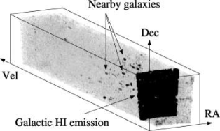
Figure 1: Orthogonal projection of HIPASS cube 93 showing emission from the Milky Way as well as other nearby galaxies. Velocity range is truncated at 10,000 km s^-1.

Initial processing of Hipass data was completed in real-time at the observatory. To correct spectra for the standard bandpass effects, spectra were reduced using the package livedata. This package also performed the conversion to heliocentric rest frame velocities by shifting spectra using Fourier techniques.

Bandpass correction is done by dividing the signal target spectrum by a reference off-source spectrum, this spectrum representing the underlying spectral shape caused by signal filtering, as well as the temperature of the receivers, ground and sky. For the Hipass data, the reference spectrum for each receiver is obtained by taking signals immediately before and after a particular integration as the telescope scans across the sky. To provide a robust measure of the bandpass, the value for each channel in the reference spectrum is taken to be the median rather than the mean of available signals. However, one artifact that can be created by this process is the generation of negative side lobes north and south of particularly bright Hi sources, since actual Hi emission is included in the bandpass determination. Finally, spectra are smoothed with a Tukey filter to suppress Gibbs ringing, resulting in a velocity resolution of 18 km s^-1.

To create the three-dimensional position-position-velocity cubes that form the main data product of Hipass, the bandpass-corrected spectra are gridded together using the package Gridzilla. The spectrum at each RA-Dec pixel is taken as the median of all data within 6 arcmin of the pixel centre, multiplied by 1.28 to correctly scale point source flux densities. This procedure thus corrupts data for extended sources in the standard Hipass data, with peak flux densities for such sources over-estimated (by 1.28 for an infinitely extended source). Extended sources nevertheless represent only a small fraction of overall sources ($\sim$2%, see Section LABEL:sec:extended) and the corresponding corrections are small. We therefore apply no correction to measured catalogue parameters for this effect. The resulting cubes from the gridding process are $\,8^{\circ}\times 8\,^{\circ}$ with $4^{\prime}\times 4^{\prime}$ pixels in the on-sky directions and extend over the full Hipass velocity range in the third axis (an example cube is shown in Figure 1). Overlap regions between cubes vary, but in general are $\sim 1\degr$ in RA and Dec. In total, 388 cubes are required to cover the southern sky.

Lastly, a correction is applied to the spectra in each Hipass data cube to minimize baseline distortion caused by the Sun and other continuum sources. This is applied using the program Luther and involves the fitting and subtraction of a template distortion spectrum.

3 The Catalogue

The Hipass Catalogue (Hicat) is compiled using a combination of automatic and interactive processes, with candidate detections first generated through automated finder scripts and then manually verified. Detections are finally parametrized using semi-automated routines. These are discussed below; a summary of the number of detections remaining at each stage is given in Table 3.

3.1 Candidate Generation

Table 3: Detection numbers at different stages of catalogue compilation

Stage	Number
Generated by MultiFind	137,060
Generated by TopHat	17,232
Examined in first two verification stages	142,276
Examined in third verification stage	61,276
Final catalogue	4,315

Table 4: Hipass parameter descriptions. Unless otherwise stated, all velocities are in the heliocentric restframe and $cz$ convention.

Figure 6: Velocity distribution of Hipass galaxies after the second verification check, with labels corresponding to potential RFI frequencies (top) and hydrogen recombination frequencies (bottom).

To identify extended sources in Hicat, all sources greater than $7^{\prime}$ in size are taken as potentially extended, this limit corresponding to 57 Jy km s^-1  from Equation LABEL:eqn:size. Assuming a uniform galaxy flux distribution, 93% of source flux is retrieved for a $7^{\prime}$ diameter source if treated as unresolved, and higher for a centrally biased distribution. In total, there are 188 candidate sources brighter than this flux limit, where flux is measured using an $44\times 44$ arcmin ‘summed’ box. Each source is examined manually, re-fitted and flagged if necessary. Where extended sources are confused or only marginally extended, detections remain fitted as point sources if this best removes erroneous flux contributions from neighbouring galaxies or cube noise. In the final catalogue, 90 sources are flagged as extended.

3.6 Interference

Figure 7: Example spectra and position-velocity maps of GPS L3 beacon

Figure 8: Example spectra and position-velocity maps of narrow-line interference

To minimize the potential effects of interference, scans in Hipass were taken in 5 separate sets, each 35 arcminutes apart, at well separated times. Nevertheless, some narrow-band interference remains in the data, the most prominent of which is a line at 1408 MHz (corresponding to $\sim 2640$ km s^-1) caused by the 11th harmonic of the 128 MHz multibeam correlator sampler clock (Barnes et al., 2001), and another line at 1400 MHz (corresponding to $\sim 4370$ km s^-1) again caused by local interference. The presence of these, along with a number of other narrow interference lines, is clearly evident in the distribution of Hicat candidates following the first two checks of the cataloguing process (top panel, Figure The HIPASS catalogue – I. Data presentation). Also apparent in the velocity distribution are detections associated with the GPS L3 beacon at 1381 MHz ($\sim 8550$ km s^-1). These detections cover a range of velocities due to intrinsic signal spreading of the GPS beacon. The presence of these interference detections following the first two verification checks is consistent with the purely spectral nature of these checks and their deliberately conservative approach to candidate rejection. However, the examination of position-velocity maps in the third stage of checking enables the removal of these false detections as shown by the final velocity distribution of the catalogue in Figure 9. The time varying nature of the GPS signal, combined with the HIPASS observation and data processing methods, results in a signal that is dominated by only a few on-sky pixels, much narrower than the signal of an unresolved source (see Figure The HIPASS catalogue – I. Data presentation). Similarly, narrow-line RFI can be distinguished by the narrow-line signature spread across large spatial regions (Figure The HIPASS catalogue – I. Data presentation).

The lack of features in the final velocity distribution at RFI frequencies shows that Hicat completeness and reliability are not significantly degraded at these locations. This point is discussed further in Section 3.5 of Paper II.

Table 5: Hydrogen $\Delta$n=1 to $\Delta$n=5 recombination lines in the range of Hipass observations (Lilley & Palmer, 1968) and their apparent Hi velocities.

Transition	Apparent Hi Velocity (km s-1)
H166a	-911
H209b	36
H239c	438
H263d	1434
H283e	1540
H240c	4199
H210b	4340
H167a	4507
H284e	4718
H264d	4857
H285e	7918
H241c	7991
H265d	8306
H211b	8685
H168a	9990
H286e	11140
H266d	11781
H242c	11815

3.7 Recombination lines

Another source of potentially erroneous Hi detections in Hicat is the recombination of warm ionized gas in the Milky Way. The full list of hydrogen $\Delta$n=1 to $\Delta$n=5 recombination lines appearing in the Hipass velocity range is given in Table 5 (taken from Lilley & Palmer, 1968) and plotted against the distribution of detections following the first two verification checks in Figure The HIPASS catalogue – I. Data presentation). Given the increased line strengths of $\Delta$n=1 transitions compared to those with higher principal quantum number differences, the erroneous detection spikes in Figure The HIPASS catalogue – I. Data presentation most likely due to hydrogen recombination are H167a and H210b. These also coincide with known RFI frequencies. Once again, these lines are successfully removed in the subsequent verification stages as demonstrated by the final source velocity distribution.

3.8 Narrow-Band Follow-up

As detailed in Paper II, an extensive program of Parkes narrow-band follow-up observations has been carried out to test the reliability of Hicat. To additionally remove as many false detections as possible, low peak flux sources and those flagged as uncertain were preferentially targetted. In total, 1082 Hicat source were confirmed in this process and 119 removed. Detections confirmed by narrow-band observations have been flagged as such in the final catalogue.

4 Data

The full data of Hicat is available on-line at:

http://hipass.aus-vo.org

This database is searchable in a number of ways, including by position and velocity. Returned parameters can be individually selected, along with any of the image products, including detection spectra, on-sky moment maps and position-velocity moment maps. The format of the returned catalogue data can also be chosen, with both HTML and plain text available. An extract of the Hipass Catalogue is given in Table 6.

We encourage other researchers to make use of this database. For optimum utility, researchers also need to be aware of the completeness, reliability and accuracy of the measured parameters. These are described in detail in Paper II. Users are also encouraged to be familiar with the full processing of Hipass data (Barnes et al., 2001).

5 Basic Property Distributions

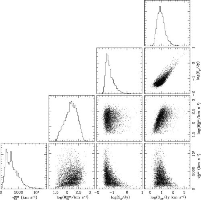
Figure 9: Log-log bivariate distributions of observed parameters: velocity ($v_{\rm 50}^{\rm max}$), velocity width ($W_{\rm 50}^{\rm max}$), peak flux ($S_{\rm p}$) and integrated flux ($S_{\rm int}$). Single parameter distributions are also given along the diagonal.

To show the basic properties of the Hipass galaxies, Figure 9 plots the bivariate distributions of velocity, velocity width, peak flux and integrated flux. Plotted along the diagonal are the one-dimensional histograms of each quantity.

The large-scale structure of the local universe is clearly visible in the velocity distribution, with two prominent over-densities appearing at $\sim$1,600 and $\sim$2,800 km s^-1. This diagram also shows the noise-limited nature of the survey, with no sharp cutoff in galaxy numbers observed at the highest observed velocities. From the peak flux distribution, it is clear that most galaxies are close to the detection limit of the survey, with the distribution peaking at $\sim$50 mJy.

The sharp decline at the upper end of the galaxy mass function can be seen by examining the peak flux-velocity and integrated flux-velocity distributions. This effective upper limit to Hi mass results in galaxies at high distances all having low peak and integrated fluxes. The steepness of the decline is apparent in the relatively sharp boundary between the flux-velocity regions in which galaxies are, and are not, observed. The low space density of the most massive galaxies is also visible in the width-velocity distribution, with small-velocity-width galaxies preferentially found nearby due to the small volumes surveyed.

Table 6. Extract of the Hipass   Catalogue. The catalogue is presented in its entirety in the electronic version of this journal. Parameter descriptions are given in Table 4. Name RA Dec $v_{\text{50}}^{\text{max}}$ $v_{\text{50}}^{\text{min}}$ $v_{\text{20}}^{\text{max}}$ $v_{\text{20}}^{\text{min}}$ $v_{\text{mom}}$ $v_{\text{Sp}}$ $v_{\text{gsr}}$ $v_{\text{lg}}$ $v_{\text{cmb}}$ $v_{\text{lo}}$ $v_{\text{hi}}$ (hrs) (deg) (km s^-1) (km s^-1) (km s^-1) (km s^-1) (km s^-1) (km s^-1) (km s^-1) (km s^-1) (km s^-1) (km s^-1) (km s^-1) $v_{\text{speclo}}$ $v_{\text{spechi}}$ $v_{\text{mask}}$ $W_{\text{50}}^{\text{max}}$ $W_{\text{50}}^{\text{min}}$ $W_{\text{20}}^{\text{max}}$ $W_{\text{20}}^{\text{min}}$ $S_{\text{p}}$ $S_{\text{int}}$ RMS RMS${}_{\text{clip}}$ RMS${}_{\text{cube}}$ cube (km s^-1) (km s^-1) (km s^-1) (km s^-1) (km s^-1) (km s^-1) (km s^-1) (Jy) (Jy km s^-1) (Jy) (Jy) (Jy) $\sigma$ box size comment follow-up confused extended (km s^-1) (arcmin) HIPASSJ0000-07 00:00:25.8 -07:49:56 3747.8 3747.8 3721.8 3721.8 3728.2 3759.8 3811.7 3870.1 3377.6 3619.0 3807.3 2210.7 5284.0 3619,3807 58.1 58.1 124.9 124.9 0.039 2.7 0.0065 0.0056 0.0115 336 158 28 1 yes no no HIPASSJ0000-40 00:00:32.3 -40:29:54 3170.8 3170.8 3169.6 3169.6 3167.9 3071.6 3138.1 3149.8 2923.4 2993.2 3342.1 1617.3 4733.8 2993,3342 239.1 239.1 258.2 258.2 0.066 12.0 0.0081 0.0063 0.0115 146 158 28 1 yes no no HIPASSJ0002-03 00:02:00.5 -03:17:01 6001.8 6001.8 6005.3 6005.3 6002.0 5966.7 6099.1 6162.8 5645.6 5917.5 6095.7 4503.7 7540.8 5918,6096 126.4 126.4 152.5 152.5 0.055 6.8 0.0064 0.0056 0.0115 337 158 28 1 no no no HIPASSJ0002-07 00:02:03.7 -07:37:56 3764.8 3764.8 3764.0 3764.0 3765.2 3773.3 3848.5 3907.1 3414.8 3714.6 3803.4 2307.5 5240.8 3715,3803 44.7 44.7 65.8 65.8 0.048 2.2 0.0073 0.0069 0.0122 286 158 28 1 yes no no HIPASSJ0002-15 00:02:29.5 -15:58:25 3416.2 3416.2 3420.8 3420.8 3422.6 3435.6 3478.1 3526.0 3089.5 3327.8 3532.2 1878.9 4971.3 3328,3532 93.6 93.6 147.1 147.1 0.039 3.7 0.0082 0.0069 0.0115 237 158 28 1 yes no no HIPASSJ0002-52 00:02:29.7 -52:47:15 1500.2 1500.2 1498.0 1498.0 1499.7 1504.6 1427.3 1419.4 1318.3 1416.3 1578.0 200.1 3030.3 1416,1578 111.4 111.4 138.1 138.1 0.051 5.6 0.0064 0.0055 0.0115 107 158 28 1 yes no no HIPASSJ0002-80 00:02:57.4 -80:20:51 1958.3 1958.3 1961.3 1961.3 1959.2 1958.3 1807.4 1758.6 1943.4 1860.9 2060.4 493.7 3424.0 1861,2060 98.7 98.7 132.8 132.8 0.242 23.4 0.0090 0.0070 0.0122 9 158 28 1 no no no HIPASSJ0004-01 00:04:46.5 -01:35:50 7194.1 7194.1 7186.9 7186.9 7186.7 7109.8 7287.7 7353.2 6829.6 7023.7 7386.3 5608.2 8795.5 7024,7386 221.4 221.4 309.4 309.4 0.046 9.4 0.0071 0.0067 0.0115 337 158 28 1 no no no HIPASSJ0005-07 00:05:12.3 -07:03:43 3810.0 3932.9 3816.1 3816.1 3817.7 3949.3 3901.3 3960.5 3467.6 3627.7 4045.7 2204.2 5432.7 3628,4046 314.8 69.1 346.6 346.6 0.086 18.0 0.0072 0.0060 0.0122 286 158 28 1 yes no no HIPASSJ0005-11 00:05:15.6 -11:29:37 6762.0 6762.0 6781.3 6756.0 6768.7 6750.8 6837.9 6891.6 6426.5 6652.8 6911.0 5239.8 8263.9 6653,6911 132.7 132.7 229.5 179.0 0.039 5.2 0.0072 0.0065 0.0122 286 158 28 1 yes no no

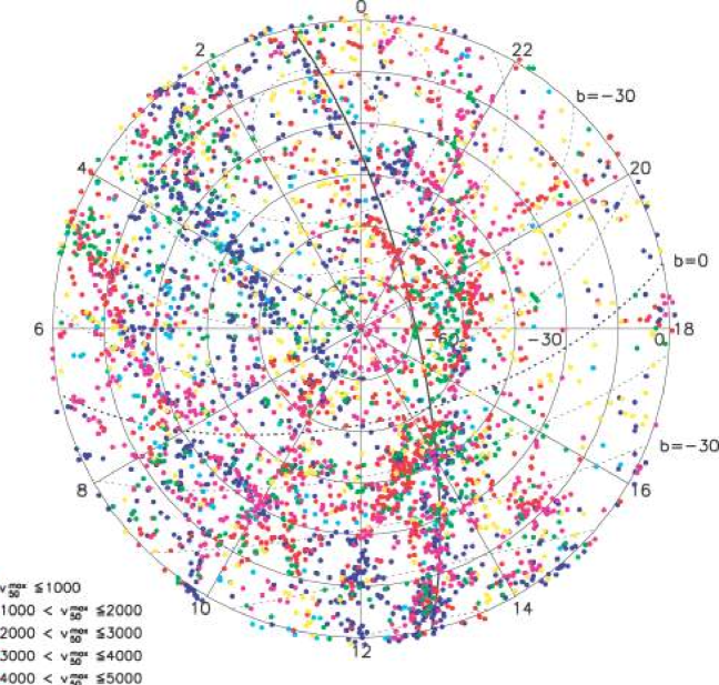
Figure 10: Polar projection of Hicat detections. Objects are colour-coded by velocity as noted in the key. Coordinate systems are marked as follows: light solid lines - equatorial coordinates; dotted lines - galactic coordinates; dark solid line - super-galactic plane.

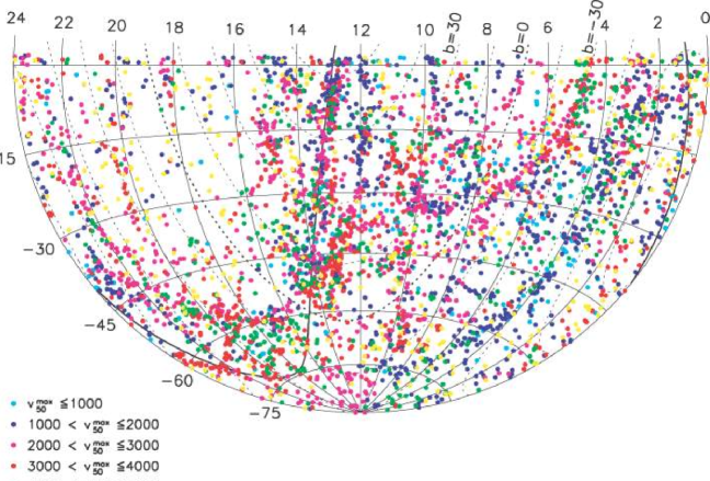
Figure 11: Aitoff projection of Hicat detections. Objects are colour-coded by velocity as noted in the key. Coordinate systems are marked as follows: light solid lines - equatorial coordinates; dotted lines - galactic coordinates; dark solid line - super-galactic plane.

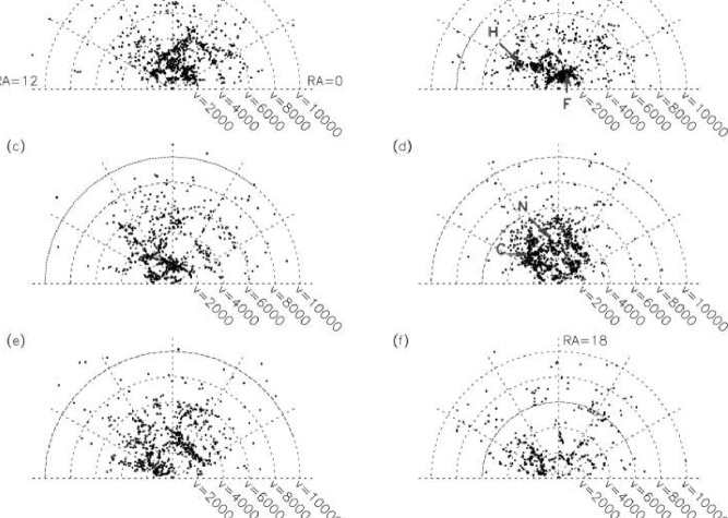
Figure 12: Velocity distribution of Hicat sources divided into segments all hinged on the equatorial plane at the 0-12 hour line starting with segment (a) with one side lying in that plane centred at RA=6hr, (b) above that and so on with (f) again with one side on the plane, but centred at RA=18hr. The location of these wedges in the southern sky is shown in Figure 14.

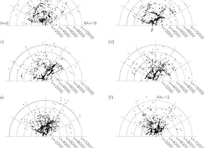
Figure 13: Velocity distribution of Hicat sources divided into segments all hinged on the equatorial plane at the 6-18 hour line starting with segment (a) with one side lying in that plane centred at RA=0hr, (b) above that and so on with (f) again with one side in the plane, but centred at RA=12hr.

Figure 14: Location in the southern sky of the velocity distribution wedges shown in Figure 12.

6 Large Scale Structure

Figures 10 and 11 plot the equatorial coordinate polar and Aitoff projections of the full on-sky distribution of Hicat sources respectively. Points are shaded according to the observed recessional velocities. From these plots, the inhomogeneous distribution of HI sources in the local universe is clearly apparent. Most obvious are the Super-Galactic plane (marked with a dark solid line), the Fornax wall (comprising the over-densities around Dorado, Fornax and Eridanus; passes through RA=3.5 hrs, Dec=$-30\degr$), and a third filament extending from near the Super-Galactic plane, through Antlia, Puppis and Lepus (passes through RA=8 hrs, Dec=$-30\degr$). Also notable are significantly under-dense regions, the most prominent of which is the Local Void (around RA=18 hrs, Dec=$-30\degr$). The location of large-scale structures is important when determining the representative nature of galaxy surveys given their search region.

Hicat also maps structures behind the Milky Way, with relatively little obscuration apparent in the observed distribution. Many of these structures and filaments have been previously identified (Kraan-Korteweg et al., 2000; Henning et al., 1998), however their uninterrupted path through the Zone of Avoidance is traced out here for the first time in a single survey.

In Figures 12 and 13, the velocity distribution of Hicat galaxies is plotted in two different projection sets. In Figure 12, the southern sky hemisphere is divided like segments of an orange into six wedges, each with a common base axis along the line RA=0-12 in the equatorial plane. The location of these wedges with respect to the southern celestial hemisphere is shown in Figure 14. The shape of these regions results in volume increasing in the vertical rather than radial direction. Thus, more galaxies are present in the central horizontal regions when compared to similar velocity regions further out. Figure 13 also divides the southern hemisphere into six wedges, this time using a common base axis along RA=6-18 in the equatorial plane.

These figures again show the Super-Galactic plane and the Local Void. Figure 12(d) contains the bulk of the Super-Galactic plane in face-on projection and Figures 13(c)-(e) show the plane in edge-on cross sections. From this second set of diagrams it is also clear that local regions of the plane are in fact comprised of two main parallel components. The lower right regions of these diagrams show the significantly under-dense region of the Local Void. Figure 12(f) most clearly shows this in the orthogonal projection in the centre of the diagram. Also marked in the velocity diagrams are the locations of four major nearby clusters (F=Fornax, C=Centaurus, H=Hydra and N=Norma), their locations coinciding with over-dense regions in the Hicat data.

7 Summary

Hipass is the first blind Hi survey of the entire southern sky. Using the Multibeam receiver on the Parkes Telescope, this survey covers $\delta<+25\degr$ with a velocity range $-$1,280 to 12,700 km s^-1. Mean noise for the survey is 13 mJy beam^-1. Taking data from the southern region of this survey $\delta<+2\degr$, we have compiled a database of 4,315 sources selected purely on their Hi content. Candidates are found using automatic finder algorithms, before being subjected to an extensive process of manual checking and verification. Issues examined in compilation of the catalogue include RFI and recombination lines, along with additional processes for confused and extended sources. A large program of follow-up observations is also used to confirm catalogue sources. Completeness, reliability and parameter accuracy of Hicat sources is addressed in Paper II. Optical counterparts to Hipass galaxies are examined in Paper III.

The large-scale distribution of sources in the catalogue covers a number of major local structures, including the Super-Galactic plane along with filaments passing through the Fornax and Puppis regions. Also notable is the probing of structure in the Zone of Avoidance, a region significantly obscured in optical bands. The survey also surveys a number of under-dense local regions including the Local Void.

This database offers a unique opportunity to study a number of important astrophysical issues. Future papers will address topics such the cosmic mass density of cool baryons, the properties of Hi selected galaxies at other wavelengths, the comparative clustering of Hi-rich galaxies, the Tully-Fisher relation, the role of hydrogen in galaxy group evolution and the study of Hi-rich galaxy environments.

8 Acknowledgments

The Multibeam system was funded by the Australia Telescope National Facility (ATNF) and an Australian Research Council grant. The collaborating institutions are the Universities of Melbourne, Western Sydney, Sydney and Cardiff, Research School of Astronomy and Astrophysics at Australian National University, Jodrell Bank Observatory and the ATNF. The Multibeam receiver and correlator was designed and built by the ATNF with assistance from the Australian Commonwealth Scientific and Industrial Research Organisation Division of Telecommunications and Industrial Physics. The low noise amplifiers were provided by Jodrell Bank Observatory through a grant from the UK Particle Physics and Astronomy Research Council. The Multibeam Survey Working Group is acknowledged for its role in planning and executing the HIPASS project. This work makes use of the AIPS++, miriad and Karma software packages. We would also like to acknowledge the assistance of Richard Gooch, Mark Calabretta, Warwick Wilson and the ATNF engineering development group. Finally, we thank Brett Beeson and the Australian Virtual Observatory for development of the SkyCat service which hosts the Hicat data.

References

- Banks et al. (1999) Banks G. D., et al., 1999, ApJ, 524, 612
- Barnes et al. (2001) Barnes D. G., et al., 2001, MNRAS, 322, 486
- Bothun et al. (1987) Bothun G. D., Impey C. D., Malin D. F., Mould J. R., 1987, AJ, 94, 23
- Braun, Thilker & Walterbos (2003) Braun R., Thilker D., Walterbos R. A. M., 2003, AAP, 406, 829
- Broeils & Rhee (1997) Broeils A. H., Rhee M.-H., 1997, A&A, 324, 877
- Cole et al. (2001) Cole S., et al., 2001, MNRAS, 326, 255
- de Vaucouleurs et al. (1991) de Vaucouleurs G., de Vaucouleurs A., Corwin H. G., Buta R. J., Paturel G., Fouque P., 1991, Third Reference Catalogue of Bright Galaxies, Springer-Verlag: Berlin Heidelberg New York
- Drinkwater et al. (2004) Drinkwater M. J., et al., 2004, Paper III, in prep.
- Fisher & Tully (1981) Fisher J. R., Tully R. B., 1981, ApJS, 47, 139
- Fixsen et al. (1996) Fixsen D. J., Cheng E. S., Gales J. M., Mather J. C., Shafer R. A., Wright E. L., 1996, ApJ, 473, 576
- Giovanelli et al. (1997) Giovanelli R., Avera E., Karachentsev I. D., 1997, AJ, 114, 122
- Haynes et al. (1999) Haynes M. P., Giovanelli R., Chamaraux P., da Costa L. N., Freudling W., Salzer J. J., Wegner G., 1999, AJ, 117, 2039
- Henning (1992) Henning P. A., 1992, ApJS, 78, 365
- Henning et al. (1998) Henning P. A., Kraan-Korteweg R. C., Rivers A. J., Loan A. J., Lahav O., Burton W. B., 1998, AJ, 115, 584
- Henning et al. (2000) Henning P. A., et al. 2000, AJ, 119, 2686
- Karachentsev & Makarov (1996) Karachentsev I. D., Makarov D. A., 1996, AJ, 111, 794
- Kerr & Henning (1987) Kerr F. J., Henning P. A., 1987, ApJ, 320, L99
- Kilborn (2001) Kilborn V. A., 2001, PhD thesis, The University of Melbourne
- Kilborn et al. (2002) Kilborn V. A., et al., 2002, AJ, 124, 690
- Koribalski et al. (2004) Koribalski B., et al, 2004, AJ, submitted
- Kraan-Korteweg et al. (2000) Kraan-Korteweg R. C., Henning P. A., Andernach H., eds, 2000, Mapping the Hidden Universe: The Universe behind the Milky Way - The Universe in HI
- Krumm & Brosch (1984) Krumm N., Brosch N., 1984, AJ, 89, 1461
- Lang et al. (2003) Lang R. H., et al., 2003, MNRAS, 342, 738
- Lilley & Palmer (1968) Lilley A. E., Palmer P., 1968, ApJS, 16, 143
- Mathewson et al. (1992) Mathewson D. S., Ford V. L., Buchhorn M., 1992, ApJS, 81, 413
- Putman et al. (2002) Putman M. E., et al., 2002, AJ, 123, 873
- Rosenberg & Schneider (2000) Rosenberg J. L., Schneider S. E., 2000, ApJS, 130, 177
- Ryan-Weber et al. (2002) Ryan-Weber E., et al., 2002, AJ, 124, 1954
- Sault et al. (1995) Sault R. J., Teuben P. J., Wright M. C. H., 1995, in ASP Conf. Ser. 77: Astronomical Data Analysis Software and Systems IV., 433
- Shostak (1977) Shostak G. S., 1977, A&A, 54, 919
- Sorar (1994) Sorar E., 1994, PhD thesis, Pittsburgh University
- Spitzak & Schneider (1998) Spitzak J. G., Schneider S. E., 1998, ApJS, 119, 159
- Staveley-Smith et al. (1996) Staveley-Smith L., et al., 1996, PASA, 13, 243
- Waugh et al. (2002) Waugh M., et al., 2002, MNRAS, 337, 641
- Zwaan et al. (1997) Zwaan M. A., Briggs F. H., Sprayberry D., Sorar E., 1997, ApJ, 490, 173
- Zwaan et al. (2004) Zwaan M. A., et al., 2004, MNRAS, Paper II, 350, 1210
- Zwaan et al. (2003) Zwaan M. A., et al., 2003, AJ, 125, 2842