The HIPASS catalogue – II. Completeness, reliability, and parameter accuracy

Abstract

The H i Parkes All Sky Survey (Hipass) is a blind extragalactic H i 21-cm emission line survey covering the whole southern sky from declination $-90^{\circ}$ to $+25^{\circ}$. The Hipass catalogue (Hicat), containing 4315 H i-selected galaxies from the region south of declination $+2^{\circ}$, is presented in Meyer et al. (2004a, Paper I). This paper describes in detail the completeness and reliability of Hicat, which are calculated from the recovery rate of synthetic sources and follow-up observations, respectively. Hicat is found to be 99 per cent complete at a peak flux of 84 mJy and an integrated flux of $9.4~{}\mbox{$\rm Jy\,km\,s^{-1}$}$. The overall reliability is 95 per cent, but rises to 99 per cent for sources with peak fluxes $>58~{}\rm mJy$ or integrated flux $>8.2~{}\mbox{$\rm Jy\,km\,s^{-1}$}$. Expressions are derived for the uncertainties on the most important Hicat parameters: peak flux, integrated flux, velocity width, and recessional velocity. The errors on Hicat parameters are dominated by the noise in the Hipass data, rather than by the parametrization procedure.

1 Introduction

The H i Parkes All Sky Survey (Hipass) is a blind neutral hydrogen survey over the entire sky south of declination $+25^{\circ}$. One of the main objectives of the survey is to extract a sample of H i-selected extragalactic objects, which can be employed to study the local large scale structure and the properties of galaxies in a manner free from optical selection effects. In Meyer et al. (2004a, paper I, hereafter) we present the Hipass sample of 4315 H i-selected objects from the region south of declination $+2^{\circ}$. This sample, which we refer to as Hicat, forms the largest catalogue of extragalactic H i-selected objects to date. In paper I the selection procedure of Hicat is described in detail, along with a discussion of the global sample properties and a description of the catalogue parameters that have been released to the public. The scientific potential of Hicat is very large, but to make optimal use of the catalogue it is essential that the completeness and reliability are well understood and quantified. Only after an accurate assessment of the completeness and reliability is it possible to extract from the observed sample the intrinsic properties of the local galaxy population.

For optically-selected galaxy samples, this procedure is relatively straightforward since most optically-selected galaxy samples are purely flux-limited, possibly complicated by the reduced detection efficiency of objects with low optical surface brightness (see e.g., Lin et al 1999, Strauss et al. 2002, Norberg et al. 2002). Since the H i 21-cm emission of galaxies is localized in a narrow region of velocity space, blind 21-cm surveys need to cover the two spatial dimensions and the velocity dimension simultaneously. The advantage of this is that the survey yields redshifts simultaneously with the object detections, and follow-up redshift surveys are not required. However, this extra dimension complicates the detection efficiency. The ‘detectability’ of a 21-cm signal depends not only on the flux, but also on how this flux is distributed over the velocity width of the signal.

In this paper we take an empirical approach to this problem, and determine the completeness of Hicat by the recovery rate of synthetic sources that have been inserted in the data. The reliability is determined by follow-up observations of a large number of sources. Our aim is to describe in detail the completeness and the reliability of Hicat as a function of various catalogue parameters, in such a way that future users can make optimal use of Hicat in studies of e.g., the H i mass function, the local large scale structure, the Tully–Fisher relation, etc. We also discuss in detail the errors on the Hicat parameters, determine expressions to estimate errors and estimate what fraction of the error is determined by noise and what fraction by the parametrization.

The organization of this paper is as follows: in Section 2 a brief review of the Hipass surveys is given. In Section 3 the completeness of Hicat is calculated using three independent methods. Section 4 details the follow-up observations and the evaluation of the reliability. In Section 5 errors on Hicat parameters are calculated.

2 The HIPASS survey

The observing strategy and reduction steps of Hipass are described in detail in Barnes et al. (2001). A full description of the galaxy finding procedure and the source parametrization is given in Paper I. Here we briefly summarize the Hipass specifics.

The observations were conducted in the period from 1997 to 2000 with the Parkes 64-m radio telescope, using the 21-cm multibeam receiver (Staveley-Smith et al. 1996). The telescope scanned strips of $8^{\circ}$ in declination and data were recorded for thirteen independent beams, each with two polarizations. A total of 1024 channels over a total bandwidth of 64 MHz were recorded, resulting in a mean channel separation of $\Delta v=13.2~{}\mbox{$\rm km\,s^{-1}$}$ and a velocity resolution of $\delta v=18~{}\mbox{$\rm km\,s^{-1}$}$ after Tukey smoothing. The data are additionally Hanning smoothed for parameter fitting to improve signal-to-noise, giving a final velocity resolution of $26.4~{}\mbox{$\rm km\,s^{-1}$}$. The total velocity coverage is $-1280$ to $12700~{}\mbox{$\rm km\,s^{-1}$}$. After bandpass calibration, continuum subtraction and gridding into $8^{\circ}\times 8^{\circ}$ cubes, the typical root-mean-square (rms) noise is $13~{}\rm mJy\,beam^{-1}$. This leads to a $3\sigma$ column density limit of $\approx 6\times 10^{17}\rm cm^{-2}$ per channel for gas filling the beam. The spatial resolution of the gridded data is $15\aas@@fstack{\prime}5$.

The basic absolute calibration method used for Hipass is described by Barnes et al. (2001). The absolute flux scale was determined during the first Hipass observations in February 1997 by calibrating a noise diode against the radio sources Hydra A and 1934-638 with known amplitudes (relative to the Baars et al. 1977 flux scale). The calibration was checked regularly (on average three time each year) by re-observing the two calibration sources. The r.m.s. of the flux measurements averaged over all 13 beams and two polarizations is 2%, which gives a good indication of the stability of the absolute flux calibration.

Two automatic galaxy finding algorithms were applied to the Hipass data set to identify candidate sources. To avoid confusion with the Milky Way Galaxy and high velocity clouds, the range $v_{\rm GSR}<300~{}\mbox{$\rm km\,s^{-1}$}$ was excluded from the list. The resulting list of potential detections was subjected to a series of independent manual checks. First, to quickly separate radio frequency interference and bandpass ripples from real H i sources, two manual checks were done examining the full detection spectra. Detections that were not rejected by both checks were then examined in spectral, position, RA-velocity, and dec-velocity space. Finally, the detections were parametrized interactively using standard miriad (Sault, Teuben,& Wright 1995) routines. This final catalogue of H i-selected sources is referred to as Hicat.

3 Completeness

The completeness $C$ of a sample is defined as the fraction of sources from the underlying distribution that is detected by the survey. For an H i-selected galaxy sample, $C$ is dependent on the peak flux, $S_{\rm p}$, and the velocity width, $W$, or alternatively on a combination of both.

One way of determining the completeness is through analytical methods. For example, for the AHISS sample presented in Zwaan et al. (1997), a ‘detectability’ parameter was calculated, which depended on the distance of the detection from the center of the beam, the variation of feed gain with frequency, the velocity width, and the integrated flux. The completeness was assumed to be 100 per cent if the detectability $>1$, corresponding to the requirement that $S_{\rm p}$ be larger that 5 times the local rms noise level after optimal smoothing. This analytically derived detectability was then compared with the survey data and proved to be a satisfactory description of the survey completeness. Rosenberg & Schneider (2002) used an empirical approach to assess the completeness of their Arecibo Dual-Beam Survey (ADBS), by inserting a large number of synthetic sources throughout the survey data. By determining the rate at which the synthetic sources could be recovered, they established the completeness, which they expressed as a function of signal-to-noise.

In this paper we also choose to assess the completeness of the Hipass sample by inserting in the data a large number of synthetic sources, prior to running the automatic galaxy finding algorithms (see Paper I). The actual process of source selection is a multi-step process, which is partly automated and partly based on by-eye verification. It is therefore preferable to study the completeness empirically instead of analytically.

The synthetic sources were constructed to resemble real sources, and were divided into three groups based on their spectral shapes: Gaussian, double-horned, and flat-topped. The sources were not spatially extended. The velocity width, peak flux, and position of each synthetic source were chosen randomly, and were drawn from a uniform parent distribution that spans the range $20$ to $650~{}\mbox{$\rm km\,s^{-1}$}$ in $W$, the range $20$ to $130$ mJy in $S_{\rm p}$, and the range $300$ to $10000~{}\mbox{$\rm km\,s^{-1}$}$ in velocity. Care was taken not to place synthetic sources on top of real sources. This was done by using the results of an automatic galaxy finding algorithm that was run prior to the insertion of the synthetic sources. A total of 1200 synthetic sources were inserted in the Hipass data cubes, with approximately equal numbers of each of the three profile types.

In Fig. 1 we show a greyscale representation of the completeness of the Hipass sample in the $S_{\rm p},W$ plane and in the $S_{\rm p},\mbox{$S_{\rm int}$}$ plane, where $S_{\rm p}$ is the peak flux density in Jy, $W$ is velocity width in $\rm km\,s^{-1}$, and $S_{\rm int}$ is the integrated flux in $\rm Jy\,km\,s^{-1}$. The completeness in these plots is simply determined by calculating $D$, the fraction of fake sources that is recovered in each bin:

$$D(S_{\rm p},W)=N^{\rm fake}_{\rm rec}(S_{\rm p},W)/N^{\rm fake}(S_{\rm p},W).$$ (1)

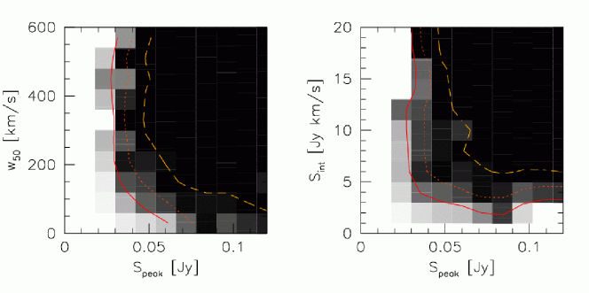
Figure 1: Bivariate completeness in the $S_{\rm p},W$ plane and the $S_{\rm p},\mbox{$S_{\rm int}$}$ plane. Darker colors correspond to higher completeness. The contours indicate completeness levels of 50, 75, and 95 per cent (from left to right).

In order to calculate the completeness as a function of one parameter, we need to integrate along one of the axes, and apply a weighting to account for the varying number of sources in each bin. Put differently, the completeness $C$ is the number of detected real sources $N$ divided by the total number of true sources in each bin, which we estimate with $N/D$. For example, the completeness as a function of $S_{\rm p}$, determined from the $S_{\rm p},W$ matrix is given by

$$C(S_{\rm p})=\frac{\sum_{W=0}^{\infty}N(S_{\rm p},W)}{\sum_{W=0}^{\infty}N(S_{\rm p},W)/D(S_{\rm p},W)}.$$ (2)

This weighting corrects for the fact that the parameter distribution of the synthetic sources might be different from that of the underlying real galaxy distribution. Similarly, $C(W)$ can be determined by integrating over $S_{\rm p}$, and $C(\mbox{$S_{\rm int}$})$ can be determined by integrating over a $S_{\rm p},\mbox{$S_{\rm int}$}$ matrix. Hereafter, we refer to $C$ as the differential completeness since it refers to the completeness at a certain value of $S_{\rm p}$, $S_{\rm int}$, or $W$.

It is often convenient to calculate the cumulative completeness $C^{\rm cum}$. For example, $C^{\rm cum}(S_{\rm p})$ is the completeness for all sources with peak fluxes larger than $S_{\rm p}$:

$$C^{\rm cum}(S_{\rm p})=\frac{\sum_{S_{\rm p}^{\prime}=S_{\rm p}}^{S_{\rm p}^{\prime}=\infty}\sum_{W=0}^{\infty}N(S_{\rm p}^{\prime},W)}{\sum_{S_{\rm p}^{\prime}=S_{\rm p}}^{S_{\rm p}^{\prime}=\infty}\sum_{W=0}^{\infty}N(S_{\rm p}^{\prime},W)/D(S_{\rm p}^{\prime},W)}.$$ (3)

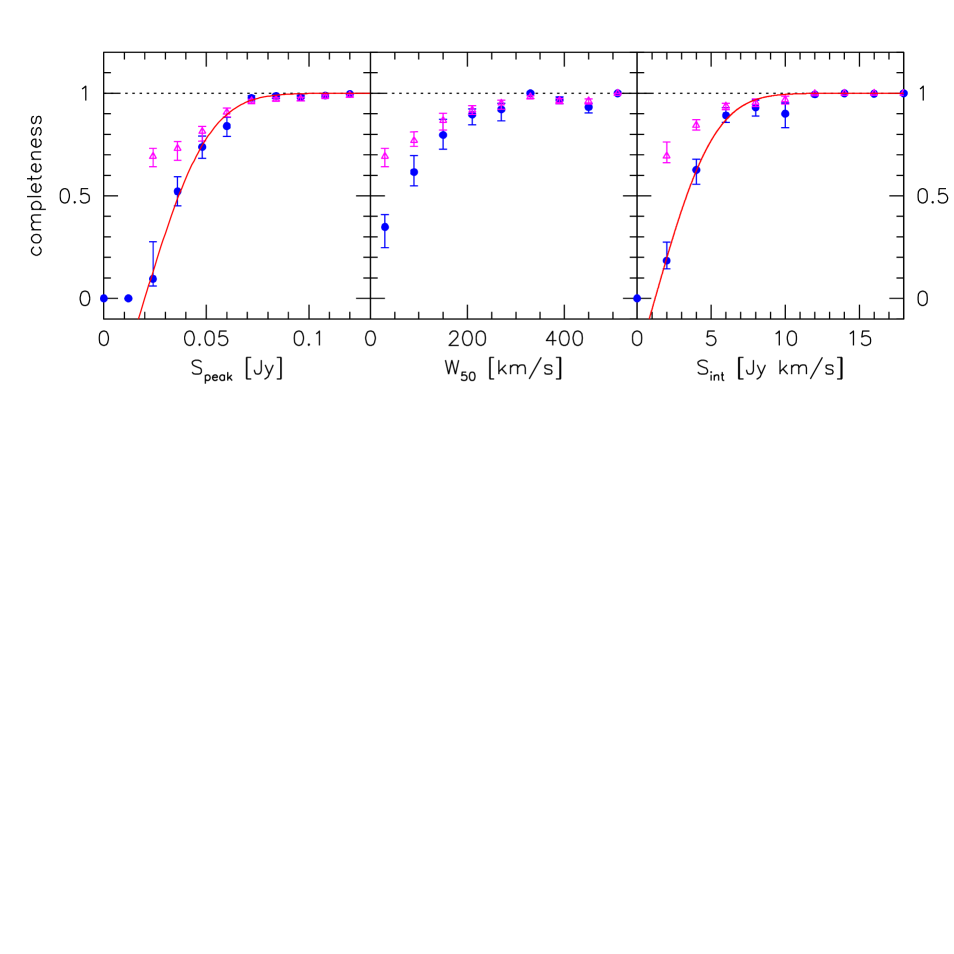
Figure 2: Completeness of Hicat as measured from the detection rate of synthetic sources. Solid circles show the differential completeness and triangles the cumulative completeness. The solid lines are error function fits to the points, with the fit parameters given in Table 1. Error bars indicate 68 per cent confidence levels.

3.1 Results

Fig. 2 shows the result of this analysis, the circles show the differential completeness as a function of $S_{\rm p}$, $W_{50}$, and $S_{\rm int}$, and the triangles show the cumulative completeness. Error bars indicate 68 per cent confidence levels and are determined by bootstrap re-sampling. We fit the completeness as a function of $S_{\rm p}$ and $S_{\rm int}$ with error functions (erf), which are indicated by solid lines. The best-fitting error functions are given in Table 1, along with the completeness limits at 95 and 99 per cent.

Table 1: Completeness

parameter	completeness	$C=0.95$	$C=0.99$
$S_{\rm p}$ (mJy)	${\rm erf}[0.028(S_{\rm p}-19)]$	68	84
$S_{\rm int}$ ($\rm Jy\,km\,s^{-1}$)	${\rm erf}[0.22(\mbox{$S_{\rm int}$}-1.1)]$	7.4	9.4
$S_{\rm p}({\rm mJy}),\mbox{$S_{\rm int}$}$($\rm Jy\,km\,s^{-1}$)	${\rm erf}[0.036(S_{\rm p}-19)]{\rm erf}[0.36(\mbox{$S_{\rm int}$}-1.1)]$

Clearly, there is not a sharp segregation between detectable and not detectable for any of the three parameters under examination. The completeness is a slowly varying function, which illustrates the complexity of the detectability of H i signals. However, all curves reach the 100 per cent completeness level. This indicates that our source finding algorithms do not miss any high signal-to-noise sources, and our system of checking all potential sources for possible confusion with RFI is sufficiently conservative that it does not cause many false negatives.

Although the above derived expressions are useful for understanding the completeness of Hicat, they do not allow us to calculate completeness levels for individual sources. For many purposes, for example in evaluating the H i mass function, it is convenient to know what the completeness of the catalogue is for a source with specific parameters. We tested different fitting functions and found that the completeness can be fitted satisfactorily using two parameters:

$$C(S_{\rm p},\mbox{$S_{\rm int}$})={\rm erf}[0.036(S_{\rm p}-19)]{\rm erf}[0.36(\mbox{$S_{\rm int}$}-1.1)].$$ (4)

This provides an accurate fit to the completeness matrices shown in Fig. 1, and also reproduces the one-parameter fits shown in Fig. 2, after the proper summation given Eq. 2 has been applied. In Fig. 3 the 50, 75, and 95 per cent completeness limits calculated using Eq. 4 are drawn on top of the parameter distribution of the full Hicat data. The contours in the $S_{\rm p},W$-plane are calculated by assuming $W=1.22\mbox{$S_{\rm int}$}/S_{\rm p}$, which provides a good fit to the data. Unfortunately, the regions of parameter space that are most densely populated are severely incomplete, as is generally true for samples that do not have a sharp completeness limit. By cutting Hicat at the 95 (99) per cent completeness limit, the sample is reduced to 2209 (1678) sources.

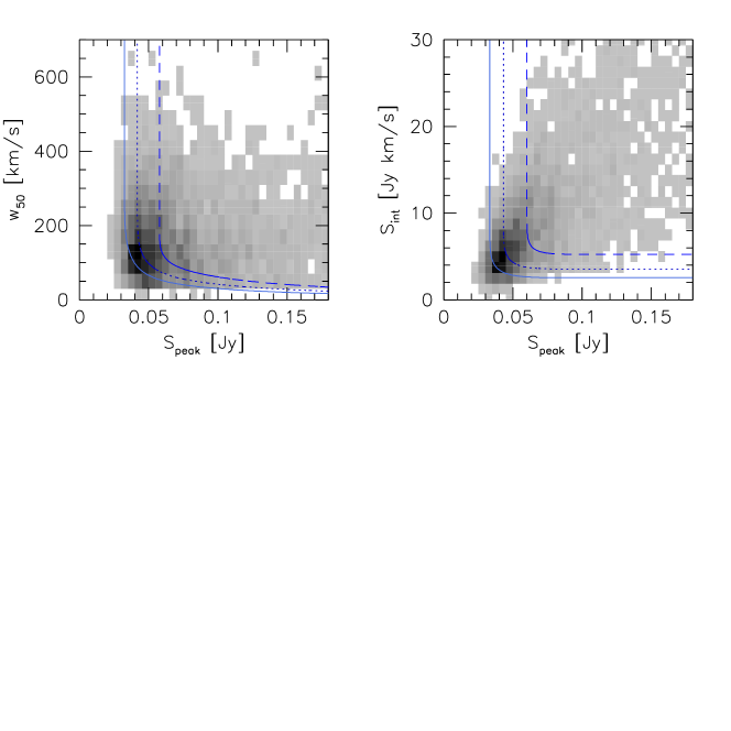
Figure 3: Bivariate parameter distribution of Hicat. Darker colors correspond to higher source densities. Analytical approximations of the completeness limits at 50, 75, and 95 per cent (from left to right) are indicated by curves.

3.2 Verification of completeness limits

Among blind extragalactic H i surveys, Hipass is unique in the sense that it is fully noise-limited. Surveys such as AHISS or the ADBS are partly bandwidth-limited, which means that the brightest galaxies in the sample can only be detected out to the distance limit set by the restricted bandwidth of the receiving system. Since Hipass is a relatively shallow survey and was conducted with a large bandwidth (64 MHz), even the detection of the most H i massive galaxies is noise-limited. The distance distribution $N(D)$ of Hicat galaxies drops to zero at large distances, before the maximum distance of $12,700~{}\mbox{$\rm km\,s^{-1}$}$ is reached (see paper I). This property of Hicat enables the use of standard techniques to verify the completeness limits determined in Section 3.1. For bandwidth-limited samples these methods would not give meaningful results.

Rauzy (2001) recently suggested a new tool to assess the completeness for a given apparent magnitude in a magnitude-redshift sample. This method is easily adapted to an H i-selected galaxy sample. Essentially, the method compares the number of galaxies brighter and fainter than every galaxy in the sample. In the case of a homogeneously distributed sample in space, the method is essentially the same as a $V/V_{\rm max}$ test, but by design Rauzy’s method is insensitive to structure in redshift space. The method is based on the definition of a random variable $\zeta$, which for a H i-selected sample can be defined as

$$\zeta=\frac{\Theta(M_{\rm HI})}{\Theta[M^{\rm lim}_{\rm HI}(Z)]},$$ (5)

where $\Theta$ is the cumulative H i mass function, $Z$ is a ‘distance modulus’ defined as $Z=\log\mbox{$S_{\rm int}$}-\log\mbox{$M_{\rm HI}$}$, and $M^{\rm lim}_{\rm HI}(Z)$ is the limiting H i mass at the distance corresponding with $Z$. An unbiased estimate of $\zeta$ for object $i$ is given by

$$\zeta_{i}=\frac{r_{i}}{n_{i}+1},$$ (6)

where $r_{i}$ is the number of objects with $\mbox{$M_{\rm HI}$}\geq\mbox{$M_{\rm HI}$}_{i}$ and $Z\leq Z_{i}$, and $n_{i}$ is the number of objects for which $\mbox{$M_{\rm HI}$}\geq\mbox{$M_{\rm HI}$}^{\rm lim}_{i}(Z_{i})$ and $Z\leq Z_{i}$. The values of $\zeta_{i}$ should be uniformly distributed between 0 and 1. Now a quantity $T_{C}$ can be defined as

$$T_{C}=\frac{\sum_{i=1}^{N_{\rm gal}}(\zeta_{i}-1/2)}{(\sum_{i=1}^{N_{\rm gal}}V_{i})^{1/2}},$$ (7)

where $V_{i}$ is the variance of $\zeta_{i}$, defined as $V_{i}=(n_{i}-1)/[12(n_{i}+1)]$. The completeness of the sample can now be estimated by computing $T_{C}$ on truncated subsamples according to a decreasing $S_{\rm int}$. For statistically complete subsamples the quantity $T_{C}$ has an expectation value of zero and unity variance. The completeness limit is found when $T_{C}$ drops systematically to negative values, where $T_{C}=-2\,(-3)$ indicates a 97.7 (99.4) per cent confidence level. In the top panel of Fig. 4 we plot the result of the $T_{C}$ completeness test. From this we derive that the completeness limit of the sample is $S_{\rm int}^{\rm lim}=9.5~{}\mbox{$\rm Jy\,km\,s^{-1}$}$ at the 97.7 per cent confidence level. This limit is very close to what was found in the previous section, where we calculated the completeness based on the detection rate of synthetic sources.

Figure 4: Test of completeness limits in Hicat. The top panel shows the $T_{C}$ estimator (see text) as a function of integrated flux. The completeness limit is reached at $\mbox{$S_{\rm int}$}=9.5~{}\mbox{$\rm Jy\,km\,s^{-1}$}$, where $T_{C}=-2$. The bottom panel shows the number of sources as a function of $S_{\rm int}$. The fitted line corresponds to the expected distribution $dN\propto S_{\rm int}^{-5/2}d\mbox{$S_{\rm int}$}$ for a flux-limited sample. The completeness limit of $\mbox{$S_{\rm int}$}=9.5~{}\mbox{$\rm Jy\,km\,s^{-1}$}$ is indicated by a vertical dashed line.

As a final verification we plot in the bottom panel of Fig. 4 the number of galaxies as a function of $S_{\rm int}$. The dotted line shows a $dN\propto S_{\rm int}^{-5/2}d\mbox{$S_{\rm int}$}$ distribution expected for a flux-limited sample, and is scaled vertically so as to fit the right hand side of the curve. Deviations from the curve start to become apparent at $\mbox{$S_{\rm int}$}=10~{}\mbox{$\rm Jy\,km\,s^{-1}$}$, which is consistent with the more accurate determination from the $T_{C}$ method. Unlike the $T_{C}$ method, this method of plotting $dN$ as a function of $S_{\rm int}$ is sensitive to the effects of large scale structure.

3.3 Completeness as a function of sky position

Hipass achieves 100 per cent coverage over the whole southern sky and has a mostly uniform noise level of $13.0\,\rm mJy\,beam^{-1}$. However, in some regions of the sky the noise level is elevated due to the presence of strong radio continuum sources. In Fig. 5 the median noise level of every Hipass cube is shown. These noise levels are determined robustly using the estimator $\sigma=s(\pi/2)^{1/2}$, where $s$ is the median absolute deviation from the median. This estimator is much less sensitive to outliers than the straight rms calculation, and provides an accurate estimate of the rms of the underlying distribution, provided that this distribution is nearly-normal. The average cube noise level is elevated more than 10 per cent over just 14.8 per cent of the sky, and elevated more than 20 per cent over 6.2 per cent of the sky. A region of elevated noise levels can be clearly identified in Fig. 5, where the highest noise values go up to $22\,\rm mJy\,beam^{-1}$. This region corresponds very closely to Galactic Plane, where the strongest radio continuum sources are located and where the density of continuum sources is highest.

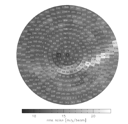
Figure 5: Median noise levels in the southern Hipass cubes. The south celestial pole is in the center, RA=0 is on top, and increases counter-clockwise. The scale bar shows the noise levels in $\rm mJy\,beam^{-1}$. The horizontal bright band corresponds to $b=0$, where the noise level is elevated. The numbers correspond to the numbers of the $8^{\circ}\times 8^{\circ}$ Hipass cubes.

It is not straightforward to assess accurately how the completeness is affected by varying noise levels. Since a significantly different noise level is only observed over a small region of the sky, the number of synthetic sources in these regions is too small to calculate the completeness limits accurately. Furthermore, the region of highest noise levels coincidently lies in the direction of the Local Void, where the detection rate of sources is naturally depressed. Therefore, the $T_{C}$ method, or a simple $V/V_{\rm max}$ method are also unreliable estimators of the completeness here. In the absence of empirical estimators, we make the reasonable assumption that the detection efficiency scales linearly with the local noise level, which means that the completeness $C(S_{\rm p})$ can be replaced with $C(S_{\rm p}\times 13.0/\sigma)$ in regions of atypical noise levels. This implies that the 95 per cent completeness level, which is normally reached at 71 mJy, is reached at 85 mJy when the noise level is elevated by 20 per cent. The completeness as a function of $W_{50}$ is probably not affected by a slight increase in noise level. The completeness as a function of $S_{\rm int}$ is adjusted similar to $C(S_{\rm p})$.

3.4 Completeness as a function of profile shape

In order to test the detection efficiency of various profile shapes, the synthetic sources were divided into three groups: Gaussian, double-horned, and flat-topped. We perform the completeness analysis for each of these subsamples individually, and show the results in Fig. 6. Within the errors, the detection efficiency as a function of peak flux is independent of profile shape. However, $C(W_{50})$ and $C(\mbox{$S_{\rm int}$})$ are somewhat depressed for double-horned profiles with respect to Gaussian and flat-topped profiles. The reason for this is probably that low signal-to-noise double-horned profiles are easily mistaken for two noise peaks, whereas Gaussian and flat-topped profiles have their flux distributed over adjoining channels, which together stand out from the noise more clearly.

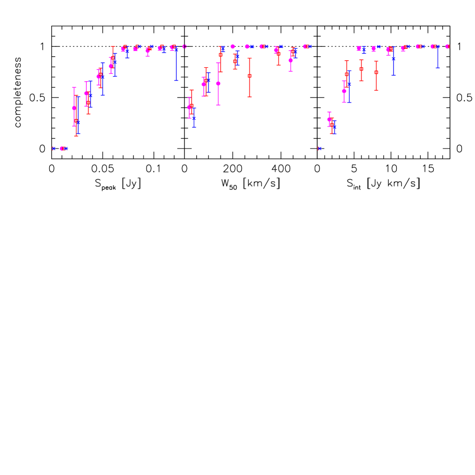
Figure 6: Completeness of Hicat as a function of profile shape. Solid circles indicate Gaussian profiles, open boxes double-horned profiles, and crosses flat-topped profiles. The points for the Gaussian and flat-topped profiles are offset horizontally to avoid overlapping of points.

3.5 Completeness as a function of velocity

In Fig. 6 of Paper I we show that the velocity distribution of the initial sample of potential Hicat detections shows strong peaks at known RFI frequencies and frequencies corresponding to hydrogen recombination lines. This might give rise to the concern that the completeness of Hicat is suppressed at these frequencies. However, in Paper I we show that the three-dimensional signature of these contaminating signals is sufficiently characteristic that they can be reliably removed from the catalogue. The final distribution of Hicat velocities shows no features that correlate with RFI or hydrogen radio recombination line frequencies, indicating that the completeness is not significantly affected at these frequencies. Unfortunately, we are not able to further substantiate this claim since 1200 uniformly distributed synthetic sources provide insufficient velocity sampling to study the completeness as function of velocity in detail.

4 Reliability

The reliability of the sample was determined by re-observing a subsample of sources with the Parkes Telescope. The aim of the observations was twofold: assessing the reliability of Hicat as a function of peak flux, integrated flux and velocity width, and removing spurious detections from the catalogue. The subsample was chosen in such a way that the full range of Hicat parameters is represented, but preference was given to those detections that have low integrated fluxes. For every observing session, a sample was created that consisted of randomly chosen Hicat detections, complemented with detections with low $S_{\rm int}$(generally lower than 8 $\rm Jy\,km\,s^{-1}$). At the time of the observations, the observer chose randomly from these samples. The full range of RA was covered by the observations.

The observations were carried out over five observing sessions between September 2001 and November 2002. They were done in narrow-band mode, which gives 1024 channels over 8 MHz, resulting in a spectral resolution of $1.65~{}\mbox{$\rm km\,s^{-1}$}$ at $z=0$. In this narrow-band correlator setting only the inner 7 beams of the multibeam system are available. An observing mode was used where the target is placed sequentially in each of the 7 beams and a composite off-source spectrum is calculated from the other 6 beams. This strategy yields a noise level $1.85$ times lower than standard on-off observations in the same amount of time. Typical integration times were 15 min. The narrow-band observations yield lower rms noise levels than standard broad-band multibeam observations. Furthermore, the high frequency resolution enables better checks of the reality of Hicat sources since narrow signals can be detected in several independent channels. The data were reduced using the AIPS++ packages livedata and gridzilla (Barnes et al. 2001), and the detections were parametrized using standard miriad routines.

First, we consider the reliability of the original catalogue, before unconfirmed sources have been taken out. The fraction of sources that was confirmed is defined as

$$T(S_{\rm p},W)=N^{\rm rel}_{\rm conf}(S_{\rm p},W)/N^{\rm rel}_{\rm obs}(S_{\rm p},W),$$ (8)

where $N^{\rm rel}_{\rm conf}$ and $N^{\rm rel}_{\rm obs}$ are the number of confirmed and observed sources, respectively. The reliability as a function of peak flux $S_{\rm p}$ is the mean of $T$, weighted by the number of sources in each bin:

$$R(S_{\rm p})=\frac{\sum_{W=0}^{\infty}N(S_{\rm p},W)\times T(S_{\rm p},W)}{\sum_{W=0}^{\infty}N(S_{\rm p},W)},$$ (9)

and the cumulative reliability is

$$R^{\rm cum}(S_{\rm p})=\frac{\sum_{S_{\rm p}^{\prime}=S_{\rm p}}^{S_{\rm p}^{\prime}=\infty}\sum_{W=0}^{\infty}N(S_{\rm p}^{\prime},W)\times T(S_{\rm p}^{\prime},W)}{\sum_{S_{\rm p}^{\prime}=S_{\rm p}}^{S_{\rm p}^{\prime}=\infty}\sum_{W=0}^{\infty}N(S_{\rm p}^{\prime},W)}.$$ (10)

Again, analogous methods can be used to measure $R(W)$ and $R(\mbox{$S_{\rm int}$})$. Fig. 7 shows the measured reliability as a function of $S_{\rm p}$, $W_{50}$, and $S_{\rm int}$. The crosses show the differential reliability, error bars indicate 68 per cent confidence levels and are determined by bootstrap re-sampling the data 200 times.

As sources that were re-observed but not confirmed were taken out of the catalogue, by re-observing a subsample of sources we improve the catalogue reliability. Eventually if we were to re-observe all sources the reliability would rise to 100 per cent. To calculate the reliability after taking out unconfirmed sources, we have to estimate the expected number of real sources, which is the number of confirmed sources plus $T$ times the number of sources that have not been observed.

A final complication arises because a second subsample of sources from Hicat was re-observed as part of a program to measure accurate velocity widths (Meyer et al. 2004b). This program also influences the reliability because non-detections were taken out of the catalogue and detections are marked as ‘confirmed’ in Hicat. This latter class of sources is indicated as $N^{\rm NB}_{\rm conf}$. Now, the expected number of real sources is given by

$$N_{\rm expreal}=N^{\rm rel}_{\rm conf}+N^{\rm NB}_{\rm conf}+(N-N^{\rm rel}_{\rm conf}-N^{\rm NB}_{\rm conf})\times(N^{\rm rel}_{\rm conf}/N^{\rm rel}_{\rm obs}).$$ (11)

Note that the total number of sources in Hicat, $N$, excludes all unconfirmed sources. Now, we can redefine $T$ as

$$T(S_{\rm p},W)=N_{\rm expreal}(S_{\rm p},W)/N(S_{\rm p},W),$$ (12)

and equations 9 and 10 can be used to calculate the reliability of Hicat. The circles and triangles in Fig. 7 show the measured differential and cumulative reliability, respectively. In total, 1201 sources were observed, of which 119 were rejected.

4.1 Results

The overall reliability is very high (95 per cent), partly because the catalogue was cleaned up considerably by re-observing many sources and rejecting unconfirmed sources from the catalogue. The reliability drops significantly below $S_{\rm p}<50$ mJy and $\mbox{$S_{\rm int}$}<5\,\rm Jy\,km\,s^{-1}$, and there is possibly a reduced reliability around $W_{50}=350~{}\mbox{$\rm km\,s^{-1}$}$. This latter feature may be related to the confusion of real H i emission signals with ripples in the spectral passband. We fit the reliability as a function of peak flux and integrated flux with error functions, the parameters of which are presented in Table 2. The 99 per cent reliability level is reached at $S_{\rm p}=58~{}\rm mJy$ and $\mbox{$S_{\rm int}$}=8.2~{}\mbox{$\rm Jy\,km\,s^{-1}$}$. If sources with a Hicat comment ‘2=have concerns’ are removed from the sample, the overall reliability rises to 97 per cent. Similarly to the results found for the completeness levels, we find that the reliability of individual sources can be determined satisfactorily as a function of $S_{\rm p}$ and $S_{\rm int}$. The functional form is given in Table 2.

Table 2: Reliability

parameter	reliability	$C=0.95$	$C=0.99$
$S_{\rm p}$ (mJy)	${\rm erf}[0.040(S_{\rm p}-12)]$	50	58
$S_{\rm int}$ ($\rm Jy\,km\,s^{-1}$)	${\rm erf}[0.12(\mbox{$S_{\rm int}$}+6.4)]$	5.0	8.2
$S_{\rm p}({\rm mJy}),\mbox{$S_{\rm int}$}$($\rm Jy\,km\,s^{-1}$)	${\rm erf}[0.045(S_{\rm p}-12)]{\rm erf}[0.20(\mbox{$S_{\rm int}$}+6.4)]$

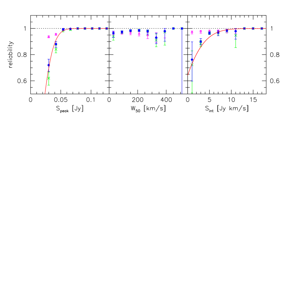
Figure 7: Reliability of Hicat measured from Parkes follow-up observations. Solid circles show the differential reliability, triangles the cumulative reliability. The crosses show the reliability of Hicat before unconfirmed sources have been taken out. The solid lines are error function fits to the points, with the fit parameters given in Table 2. Error bars indicate 68 per cent confidence levels.

5 Parameter uncertainties

A detailed description of all measured parameters in Hicat is presented in Paper I. Here we discuss the error estimates of the most important parameters: peak flux, integrated flux, velocity width, heliocentric recessional velocity ($cz$) and sky position. Other authors have discussed analytical approaches to estimating uncertainties on H i 21-cm parameters (e.g., Schneider et al. 1990, Fouqué et al. 1990, Verheijen & Sancisi 2001), but for Hicat  sufficient comparison data are available to measure the errors empirically. In this analysis we make use of the synthetic source parameters and the narrow-band observations to determine the total observational errors on the parameters. The data published in the Hipass BGC (Koribalski et al. 2004) are used to establish what fraction of the error is caused by the parametrization procedure.

We assume that the error $\sigma_{X}$ on parameter $X$ can be satisfactorily described by

$$\sigma(X)=c_{1}Y^{n}+c_{2},$$ (13)

where $Y$ is a parameter that can be equal to $X$ or any other parameter, and $n$, $c_{1}$, and $c_{2}$ are constants. There is no physical basis for this analytical description of the errors, but we find later that Eq. 13 provides satisfactory fits to the measured parameter uncertainties. In the following we determine how each $\sigma(X)$ depends on all parameters.

When comparing parameters from different data sets, we know that the measured rms scatter on the difference between Hicat parameter $X$ and parameter $X$ from data set $Z$ is given by

$$\sigma(X)_{\rm meas}^{2}=\sigma(X)_{\rm HICAT}^{2}+\sigma(X)_{\rm Z}^{2},$$ (14)

where $\sigma(X)_{\rm meas}$ is the measured rms scatter on $X_{\rm HICAT}-X_{\rm Z}$, $\sigma(X)_{\rm HICAT}$ is the error in the Hicat parameter, and $\sigma(X)_{\rm Z}$ is the error in data set $Z$. The latter two parameters are unknown, but we can make the simplifying assumption that

$$\sigma(X)_{\rm Z}=\sigma(X)_{\rm HICAT}\frac{\rm rms_{\rm Z}}{\rm rms_{\rm HICAT}}$$ (15)

where $\rm rms_{\rm Z}$ denotes the rms noise in the survey on which catalogue $Z$ is based.

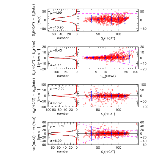
Figure 8: Comparison between Hicat and synthetic source parameters. The left panels show the histograms of the differences, which are fitted by Gaussian profiles for which the parameters are indicated in the top left corners. The right panels show the differences as a function of the measured Hicat parameters. The points and error bars show the zero-points and the widths of the fitted Gaussians (inner and outer error bars indicate $1\sigma$ and $3\sigma$, respectively). The dashed lines are the best-fitting analytical descriptions of $3\sigma(X)$.

5.1 Error estimates from comparison with synthetic sources

First, we compare the Hicat parameters with those of the synthetic sources. This comparison is particularly useful for estimating errors because the synthetic source parameters are noise free, which means that $\sigma(X)_{\rm fake}=0$ for all parameters. Therefore, the measured $\sigma(X)_{\rm meas}$ is equal to $\sigma(X)_{\rm HICAT}$, which is the parameter of interest. In Fig. 8 we plot the difference between the measured Hicat parameters and parameters of the synthetic sources that were inserted into the data. The left panels show the difference histograms, fitted by Gaussian profiles. Parameters for these are indicated in the top left corners. The right panels show the differences as a function of the measured Hicat parameters. The points and error bars show the zero-points and widths of the fitted Gaussians (inner and outer error bars indicate $1\sigma$ and $3\sigma$, respectively) in different bins. We prefer Gaussian fitting to calculating straight rms values because this latter estimator is much more sensitive to outliers. In the right panels we indicate the best-fitting relations for $3\sigma(X)$ by dashed lines.

As is expected, the error on $S_{\rm p}$ is independent of peak flux. The measurement error is just determined by the 13.0 mJy rms noise in the spectra, but lowered to a measured value of 11.0 mJy due to the fact that more than one channel may contribute to the measurement of $S_{\rm p}$. The error on $S_{\rm p}$ is not found to be dependent on any of the other parameters, so we adopt a fixed value of $\sigma(\mbox{$S_{\rm p}$})=11.0\,\rm mJy$. The other effect than can be seen in this panel is that there is a global offset of 5.0 mJy in the measured $S_{\rm p}$ with respect to the peak flux of the synthetic sources. This effect, which in Zwaan et al. (2003) is referred to as the ‘selection bias’, arises because after adding noise to a spectrum the measured peak flux density is generally an overestimation of the true peak flux density.

The error in $S_{\rm int}$ is found to be dependent on $S_{\rm int}$ only, and can be satisfactorily fitted with $c_{1}=0.5$, $n=1/2$. This implies that $\sigma(\mbox{$S_{\rm int}$})=1.5~{}\mbox{$\rm Jy\,km\,s^{-1}$}$ (or 16 per cent) at the 99 per cent completeness limit of $9.4~{}\mbox{$\rm Jy\,km\,s^{-1}$}$. Fouqué et al. (1990) derive that $\sigma(\mbox{$S_{\rm int}$})$ is dependent on both $S_{\rm int}$ and $S_{\rm p}$ as $\sigma(\mbox{$S_{\rm int}$})\propto\mbox{$S_{\rm int}$}^{1/2}\mbox{$S_{\rm p}$}^{-1/2}$. Our analysis shows that for the Hicat data $\sigma(\mbox{$S_{\rm int}$})$ can be described satisfactorily as a function of $S_{\rm int}$ only. The error in $S_{\rm int}$ will be the dominant factor in the error on the H i mass, except for the nearest galaxies for which peculiar velocities contribute significantly to the uncertainty in H i mass.

The error in $W_{50}$ is not clearly dependent on any other parameter, so we adopt a constant $\sigma(W_{50})=7.5\,\rm kms^{-1}$. It should be noted, however, that there appears to be an excess of points which is not satisfactorily fitted with a single Gaussian. These outliers are preferentially those with low peak fluxes, but large velocity widths. Larger uncertainties in the measurements of velocity width occur with broad, low signal-to-noise profiles, because the edges of the profiles can not always be chosen unambiguously. Approximately one-third of the measurements can be fitted with a Gaussian with $\sigma=25\,\rm km\,s^{-1}$.

We find that the error on recessional velocity is dependent on $S_{\rm p}$ only, with higher peak flux detections having lower errors on the measured $V_{\rm hel}$. The error bars can be fitted with parameters $c_{1}=1.0\times 10^{4}$, $n=-2$ and $c_{2}=5$. Fouqué et al. (1990) find for their data that $n=-1$, but incorporate an additional dependence on the steepness of the H i profile.

In Fig. 9 the top panel shows the difference between position of the inserted synthetic sources and the fitted position after parametrization. The lower two panels show the position differences as a function of $S_{\rm int}$. The positional accuracy in RA is fitted with $c_{1}=5.5$, $n=-1$, $c_{2}=0.45$, and the accuracy in Dec is fitted with $c_{1}=4$, $n=-1$, $c_{2}=0.4$. These numbers imply that the positional accuracy at the 99 per cent completeness limit is $1\aas@@fstack{\prime}05$ in RA, and $0\aas@@fstack{\prime}82$ in Dec. The difference between these two numbers arises because the Hipass data are more regularly sampled in the Dec direction (see Barnes et al. 2001). This positional accuracy agrees very well with the results found from Hicat matching with the 2MASS Extended Source Catalogue (Jarret et al. 2003, see Meyer et al. 2004b).

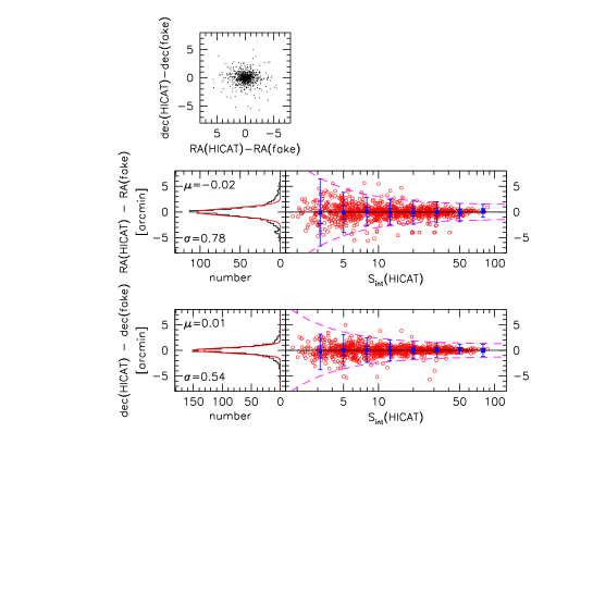
Figure 9: The top panel shows the difference between the position of the inserted synthetic sources and the fitted position after parametrization, in arcmin. The lower panels are similar to those in Fig. 8.

Table 3: Parameter uncertainties

parameter	error	$\sigma$ at $C=0.99$
$\sigma(S_{\rm p})$	$11.0\,\rm mJy$	$11.0\,\rm mJy$
$\sigma(\mbox{$S_{\rm int}$})$	$0.5S_{\rm int}^{1/2}\,\mbox{$\rm Jy\,km\,s^{-1}$}$	$1.5\,\mbox{$\rm Jy\,km\,s^{-1}$}$
$\sigma(W_{50})$	$7.5\,\rm km\,s^{-1}$	$7.5\,\rm km\,s^{-1}$
$\sigma(V_{\rm hel})$	$1.0\times 10^{4}S_{\rm p}^{-2}+5\,\rm km\,s^{-1}$	$6.4\,\rm km\,s^{-1}$
$\sigma(\rm RA)$	$5.5S_{\rm int}^{-1}+0.45\,\rm arcmin$	$1.05\,\rm arcmin$
$\sigma(\rm dec)$	$4S_{\rm int}^{-1}+0.4\,\rm arcmin$	$0.82\,\rm arcmin$

5.2 Verification of error calculations with Parkes follow-up observations

Although the comparison with noise-free parameters in the previous subsection is a useful method of estimating the errors on Hicat parameters, it is important to verify these results with independent measurements. Such measurement are available through our program of Parkes narrow-band (NB) follow-up observations, which was described in Section 4. These follow-up observations are preferentially targeted at sources with low integrated fluxes, but the sample is sufficiently large to make a meaningful parameter comparison over a large dynamic range. The NB observations were carried out independently from the Hipass program and consisted of pointed observations instead of the active scanning used for Hipass. The spectral resolution of the NB observations was 1.65 $\rm km\,s^{-1}$, compared to 13.2 $\rm km\,s^{-1}$ for Hipass, but the data used in this section were smoothed to the Hipass resolution. The NB profiles were parametrized with the same miriad software used for Hicat.

In Fig. 10 the differences between Hicat parameters and those from follow-up observations is presented. The dashed lines in the right-hand panels are not fits to the error bars, but are the equations given in Table 3, converted using Eq. 14 and Eq. 15. Here we have adopted ${\rm rms}_{\rm NB}=7\,\rm mJy$, which is the mean rms noise in the follow-up spectra after smoothing these to the Hipass resolution. The converted error estimates provide good fits to the measured scatter, indicating that the equations in Table 3 can be used to find reliable errors on Hicat parameters. We note that the errors on the peak and integrated flux include the uncertainties in the calibration of the flux scale, except for errors in the Baars et al. (1977) flux scale.

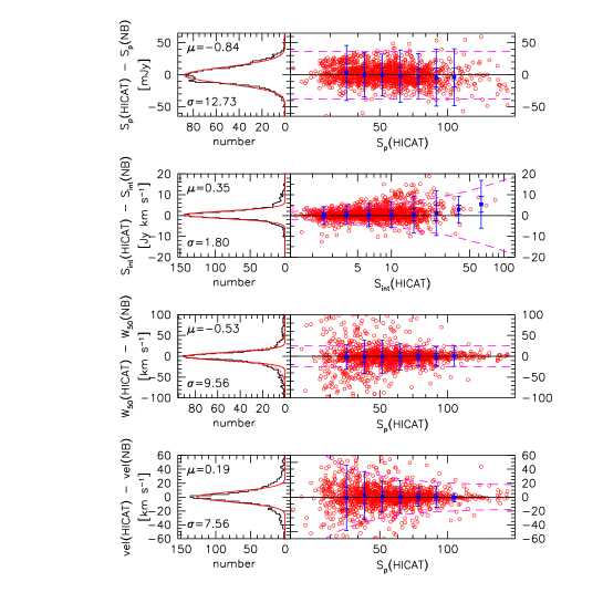
Figure 10: Similar to Fig. 8, but showing the comparison between parameters from Hicat and narrow-band follow-up observations.

5.3 Parameter comparison with Bright Galaxy Catalogue

The Bright Galaxy Catalogue (BGC, Koribalski et al. 2004) consists of the 1000 Hipass galaxies with the highest peak fluxes and is assembled and parametrized independently from Hicat, but is extracted from the same data cubes. By comparing the Hicat parameters with those from the BGC, it can be determined what fraction of the error on the Hicat parameters is determined by the parametrization procedure (internal error), and what fraction is caused by noise in the Hipass data (external error). This comparison is particularly interesting because generally in the parametrization of a 21-cm emission line profile a number of choices are made, which could differ between the persons doing the parametrization. The biggest uncertainty is probably the fitting and subtracting of the spectral baseline. Structure in the baseline is caused by ringing associated with strong Galactic H i emission and continuum emission that can produce standing wave patterns in the telescope structure. For the BGC, the spectral baselines were fitted with polynomials, of which the order is a free parameter, whereas Hicat baselines were fitted with Gaussian smoothing, where the dispersion is a free parameter (see paper I). Another uncertainty is introduced with the choice of the velocity extrema of line profiles, between which the flux is integrated.

In Fig. 11 the comparison with the BGC is shown. The difference between Hicat and BGC parameters is very small. There are no systematic trends, except for a slight excess of points with high values of $\mbox{$S_{\rm int}$}({\rm HICAT})-\mbox{$S_{\rm int}$}({\rm BGC})$ at large values of $S_{\rm int}$. This excess arises because Hicat and the BGC use different criteria to define what is an extended source. This leads to more sources in Hicat being fitted as extended, which generally results in higher values of $S_{\rm int}$. Overall, we find that the parametrization error contributes only marginally to the total error, with a contribution of 8 per cent to $\sigma(S_{\rm p})$, 13 per cent to $\sigma(\mbox{$S_{\rm int}$})$, and 1 per cent to $\sigma(W_{50})$. The contribution to $\sigma(V_{\rm hel})$ is not uniquely defined because it depends on $S_{\rm p}$, but on average it is 13 per cent. The rms scatter on the difference between the BGC and Hicat values of $V_{\rm hel}$ is only $4.8~{}\mbox{$\rm km\,s^{-1}$}$ at the 99 per cent completeness limit and drops to $2~{}\mbox{$\rm km\,s^{-1}$}$ for brighter sources.

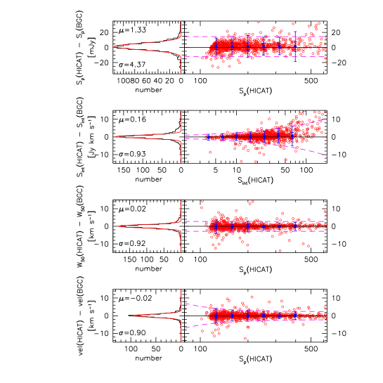
Figure 11: Similar to Fig. 8, but showing the comparison between parameters from Hicat and the Hipass Bright Galaxy Catalogue (Koribalski et al. 2004).

6 Summary

The full catalogue of extragalactic Hipass detections (Hicat) has now been released to the public (Meyer et al. 2004a, paper I). In the present paper we have addressed in detail the completeness and reliability of the survey. We present analytical expressions that can be used to approximate the completeness and reliability. We find that Hicat is 99 per cent complete at a peak flux of 84 mJy and an integrated flux of $9.4~{}\mbox{$\rm Jy\,km\,s^{-1}$}$. The overall reliability is 95 per cent, but rises to 99 per cent for sources with peak fluxes $>58~{}\rm mJy$ or integrated flux $>8.2~{}\mbox{$\rm Jy\,km\,s^{-1}$}$. Expressions are derived for the uncertainties on the most important Hicat parameters: peak flux, integrated flux, velocity width, and recessional velocity. The errors on Hicat parameters are dominated by the noise in the Hipass data, rather than by the parametrization procedure.

References

- [] Baars, J. W. M., Genzel, R., Pauliny-Toth, I. I. K., & Witzel, A. 1977, A&A, 61, 99
- [] Barnes, D. G. et al. 2001, MNRAS, 322, 486
- [Fouque et al.(1990)] Fouqué, P., Durand, N., Bottinelli, L., Gouguenheim, L., & Paturel, G. 1990, A&AS, 86, 473
- [] Jarret, T. H, Chester, T., Cutri, R., Schneider, S. E., Huchra, J. P. 2003, AJ, 125, 525
- [] Koribalski, B. S. et al. 2004, submitted to AJ
- [Lin et al.(1999)] Lin, H., Yee, H. K. C., Carlberg, R. G., Morris, S. L., Sawicki, M., Patton, D. R., Wirth, G., & Shepherd, C. W. 1999, ApJ, 518, 533
- [] Meyer, M. J., Zwaan, M. A., Webster, R. L., Staveley-Smith, L., et al. 2003a (paper I), submitted to MNRAS
- [] Meyer, M. J., et al. 2004b, in preparation
- [Norberg et al.(2002)] Norberg, P. et al. 2002, MNRAS, 336, 907
- [] Rauzy, S. 2001, MNRAS, 324, 51
- [] Rosenberg, J. L. & Schneider, S. E. 2002, ApJ, 567, 247
- [] Sault R. J., Teuben P. J., & Wright M. C. H., 1995, in Astronomical Data Analysis Software and Systems IV, ed. R. Shaw, H.E. Payne, J.J.E. Hayes, ASP Conf. Ser., 77, 433-436
- [Schneider, Thuan, Magri, & Wadiak(1990)] Schneider, S. E., Thuan, T. X., Magri, C., & Wadiak, J. E. 1990, ApJS, 72, 245
- [] Staveley-Smith, L. et al. 1996, Publications of the Astronomical Society of Australia, 13, 243
- [Strauss et al.(2002)] Strauss, M. A. et al. 2002, AJ, 124, 1810
- [Verheijen & Sancisi(2001)] Verheijen, M. A. W. & Sancisi, R. 2001, A&A, 370, 765
- [] Zwaan, M. A., Briggs, F. H., Sprayberry, D., & Sorar, E. 1997, ApJ, 490, 173
- [] Zwaan M. A., Staveley-Smith L., Koribalski B. S., et. al. 2003, AJ, 125, 2842