Constraints on mode couplings and modulation of the CMB with WMAP data.

Abstract

We investigate a possible asymmetry in the statistical properties of the cosmic microwave background temperature field and to do so we construct an estimator aiming at detecting a dipolar modulation. Such a modulation is found to induce correlations between multipoles with $\Delta\ell=1$. Applying this estimator, to the V and W bands of the WMAP data, we found a significant detection in the V band. We argue however that foregrounds and in particular point sources are the origin of this signal.

I Introduction

The Wilkinson Microwave Anisotropy Probe (WMAP) data [1, 2] have raised a number of interrogations concerning the statistical properties of the temperature field. While these data globally confirm the standard inflationary paradigm [3] and the concordance cosmological model, they exhibit some intriguing anomalies, particularly concerning the large angular scales. In particular, a huge activity has been devoted to the study of the low value of the quadrupole and octopole [4, 5, 6, 7] as well as their alignment [8, 9], two effects that appear to be inconsistent with the standard cosmological model.

Besides, many authors have tried to test the statistical properties of the temperature field using various methods. For instance, it was investigated whether the coefficients $a_{\ell m}$ of the development of the temperature field on spherical harmonics were independent and Gaussian distributed. While, as expected from the standard inflationary picture, a $\chi^{2}$ deviation from Gaussianity seems to be well constrained [10], there have been some claims that the distribution may not be isotropic [9, 11, 12, 13, 14, 15] or Gaussian [16, 17, 18, 19]. No real physical understanding of these measurements have been proposed yet and the origin of these possible features is still unknown. Some authors have argued in favor of systematic effects [13] while it was argue [14, 20] that foreground contamination may play an important role in these conclusions.

From a theoretical point of view, there are many reasons to look for (and/or constrain) a departure from Gaussianity and/or isotropy of the CMB temperature field. Mode correlation can be linked to non-Gaussianity, in particular due to finite size effects [21, 22, 23] or to the existence of some non-trivial topology of the universe [25]. While in the latter case, one expects to have a complex correlation matrix of the $a_{\ell m}$, the former leads generically to a dipolar modulation of the CMB field [24]. Such a modulation induces in particular correlations between adjacent multipoles ($\Delta\ell=1$). Similar correlations but with $\Delta\ell=2$ may also be induced by a primordial magnetic field [26]. In each case, the physical model and its predictions indicate the type of correlations to look for and will drive the design of an adapted estimator.

Investigation of the correlation properties of $a_{\ell m}$ is thus important to correctly interpret previous observational results [9, 11, 12, 13, 14, 15]. Two approaches are thus possible. Either one defines some general estimators and study whether they agree with a Gaussian and isotropic distribution (top-down approach) or one sticks to a class of physical models and construct an adapted estimator (bottom-up approach). In this article, we follow the second route and focus to the task of constraining a possible dipolar modulations of the CMB temperature field, that is correlations between multipoles with $\Delta\ell=1$.

In Section II, we start by some general considerations on the form of the correlation arising from a dipolar modulation. We then built an estimator, in Section III, adapted to these types of correlations. In particular, we cannot use full-sky data and we will need to cut out some part of the sky. The effect of such a mask on the correlations will have to be taken into account and included in the construction of the estimator. We apply this estimator to the V and W bands of the WMAP data in Section IV. The V band exhibits an apparent detection. The interpretation of this result will require us to compare various masks, and in particular to investigate the effect of point sources on the signal to conclude that they are most likely its cause.

II General considerations

As explained in the introduction, we focus on a possible dipolar modulation of the CMB signal. Thus, we assume that the observed temperature field can be modelled as

$${\Theta^{\rm obs}}({\vec{\gamma}})=\Theta({\vec{\gamma}})\left[1+{\varepsilon_{-1}}Y_{1,-1}({\vec{\gamma}})+{\varepsilon_{0}}Y_{1,0}({\vec{\gamma}})+{\varepsilon_{+1}}Y_{1,+1}({\vec{\gamma}})\right]$$ (1)

where $\Theta$ is the genuine statistically isotropic field and where $({\varepsilon_{-1}},{\varepsilon_{0}},{\varepsilon_{+1}})$ are three unknown parameters that characterizes the direction of the modulation. The modulation has to be real so that ${\varepsilon_{0}}$ is real and ${\varepsilon_{+1}}=-{\varepsilon_{-1}}^{*}\equiv\varepsilon$.

As usual, we decompose the temperature fluctuation in spherical harmonics as

$$\Theta({\vec{\gamma}})=\sum_{\ell=2}^{\infty}\sum_{m=-\ell}^{\ell}a_{\ell m}Y_{\ell,m}({\vec{\gamma}}).$$ (2)

The coefficients $a_{\ell m}$ are thus given by

$$a_{\ell m}=\int{\rm d}^{2}{\vec{\gamma}}\Theta({\vec{\gamma}})Y_{\ell,m}^{*}({\vec{\gamma}}).$$ (3)

${\Theta^{\rm obs}}$ and $a_{\ell m}^{\rm obs}$ are defined and related in the same way. Since $\Theta$ is supposed to be the primordial, Gaussian and statistically isotropic, temperature field, its correlation matrix reduces to

$$\left<a_{\ell m}\,a_{\ell^{\prime}m^{\prime}}^{*}\right>=C_{\ell}\delta_{\ell\ell^{\prime}}\delta_{mm^{\prime}}.$$ (4)

A modulation of the form (1) implies that the coefficients $a_{\ell m}^{\rm obs}$ develop correlations between multipoles with $\Delta\ell=1$. Let us illustrate the origin of this correlation. From Eqs. (1) and (4), we deduce that

$$a_{\ell m}^{\rm obs}=a_{\ell m}+\sum_{\ell^{\prime}=2}^{\infty}\sum_{m^{\prime}=-\ell^{\prime}}^{\ell^{\prime}}a_{\ell^{\prime}m^{\prime}}\sum_{i=-1}^{+1}\varepsilon_{i}\int{\rm d}^{2}{\vec{\gamma}}Y_{\ell,m}^{*}({\vec{\gamma}})Y_{\ell^{\prime},m^{\prime}}({\vec{\gamma}})Y_{1,i}({\vec{\gamma}}).$$ (5)

The integral can be easily computed by using the Gaunt formula [see Eq. (79)] to get

$$a_{\ell m}^{\rm obs} = a_{\ell m}+\sqrt{\frac{3}{4\pi}}\sum_{i}\varepsilon_{i}(-1)^{m}\sum_{LM}\,a_{LM}\,\sqrt{(2\ell+1)(2L+1)}\left(\begin{array}[]{ccc}\ell&L&1\\ -m&M&i\end{array}\right)\left(\begin{array}[]{ccc}\ell&L&1\\ 0&0&0\end{array}\right).$$ (10)

Because of the triangular inequality, the Wigner $3j$-symbols are non zero only when $L=\ell\pm 1$ and $M=m-i$ so that $a_{\ell m}^{\rm obs}$ is in fact a sum involving $a_{\ell m}$ and $a_{\ell\pm 1m-i}$. It follows that it will develop $\ell-(\ell+1)$ correlations that can be characterized by the two quantities

$$D_{\ell m}^{(0)} \equiv \left<a_{\ell m}^{\rm obs}\,a_{\ell+1m}^{{\rm obs}*}\right>,$$ (11)

$$D_{\ell m}^{(1)} \equiv \left<a_{\ell m}^{\rm obs}\,a_{\ell+1m+1}^{{\rm obs}*}\right>$$ (12)

which will be non zero respectively as soon as ${\varepsilon_{0}}$ or $\varepsilon$ are non zero. Using the expression (10) and the property (4) of the primordial field, we deduce that

$$D_{\ell m}^{(0)}={\varepsilon_{0}}\,\sqrt{\frac{3}{4\pi}}\,\frac{\sqrt{(\ell+1)^{2}-m^{2}}}{\sqrt{(2\ell+1)(2\ell+3)}}\,\left(C_{\ell}+C_{\ell+1}\right)$$ (13)

$$D_{\ell m}^{(1)}=\sqrt{\frac{3}{4\pi}}\,\sqrt{\frac{(\ell+2+m)(\ell+1+m)}{(2\ell+1)(2\ell+3)}}\,\left[C_{\ell}+C_{\ell+1}\right]\frac{\varepsilon^{*}}{\sqrt{2}}.$$ (14)

Interestingly, these forms indicate how to sum the $D_{\ell m}$ in order to construct an estimator. This construction will be detailed in the following section.

III Mathematical construction of the estimator

The previous analysis is illustrative but not suitable to be applied on real data. In particular these data will not be full sky and we have to take into account the effect of a mask (see e.g. Ref. [27]). Such a mask, that arises in particular because of the galactic cut, will induce correlations in the coefficients $a_{\ell m}^{\rm obs}$ that are described in § III.1. We design the mask in order to protect the correlations that originate from the modulation (§ III.2 and § III.3) and finish by presenting the construction of our estimator in the most general case (§ III.4).

III.1 Mask effects

The temperature field is observed only on a fraction of the sky. We thus have to mask part of the map so that the temperature field is in fact given by

$${\Theta^{\rm obs}}({\vec{\gamma}})=\Theta({\vec{\gamma}})\left[1+\sum_{i=-1}^{1}\varepsilon_{i}Y_{1,i}({\vec{\gamma}})\right]W({\vec{\gamma}})$$ (15)

where $W({\vec{\gamma}})$ is a window function, referred to as mask, indicating which part of the sky has been cut. We decompose $W({\vec{\gamma}})$ in spherical harmonics as

$$W({\vec{\gamma}})=\sum_{\ell m}\,w_{\ell m}\,Y_{\ell m}({\vec{\gamma}}).$$ (16)

$W({\vec{\gamma}})$ being a real valued function, it implies that $w_{\ell m}^{*}=(-1)^{m}w_{\ell-m}$. We deduce from Eqs. (15) and (3) that

$$a_{\ell m}^{\rm obs}=\widetilde{a}_{\ell m}+\sum_{i}\varepsilon_{i}A^{(i)}_{\ell m}$$ (17)

where $\widetilde{a}_{\ell m}$ are the coefficients of the masked primordial temperature field $\widetilde{\Theta}({\vec{\gamma}})=\Theta({\vec{\gamma}})W({\vec{\gamma}})$,

$$\widetilde{a}_{\ell m}=\sum_{{\ell_{1}}{m_{1}}}\,a_{{\ell_{1}}{m_{1}}}\sum_{{\ell_{2}}{m_{2}}}\,w_{{\ell_{2}}{m_{2}}}\int{\rm d}^{2}{\vec{\gamma}}\,Y_{{\ell_{1}}{m_{1}}}({\vec{\gamma}})Y_{{\ell_{2}}{m_{2}}}({\vec{\gamma}})Y_{\ell,m}^{*}({\vec{\gamma}})$$ (18)

and the effects of the modulation are encoded in the correction

$$A^{(i)}_{\ell m}=\sum_{{\ell_{1}}{m_{1}}}\,a_{{\ell_{1}}{m_{1}}}\sum_{{\ell_{2}}{m_{2}}}\,w_{{\ell_{2}}{m_{2}}}\int{\rm d}^{2}{\vec{\gamma}}\,Y_{{\ell_{1}}{m_{1}}}({\vec{\gamma}})Y_{{\ell_{2}}{m_{2}}}({\vec{\gamma}})Y_{1i}({\vec{\gamma}})Y_{\ell,m}^{*}({\vec{\gamma}}).$$ (19)

Interestingly, $\widetilde{a}_{\ell m}$ can be shown to be obtained from $a_{\ell m}$ by the action of a Kernel $K_{\ell m}^{{\ell_{1}}{m_{1}}}$

$$\widetilde{a}_{\ell m}=\sum_{{\ell_{1}}{m_{1}}}\,a_{{\ell_{1}}{m_{1}}}K_{\ell m}^{{\ell_{1}}{m_{1}}}.$$ (20)

This kernel is defined by

$$K_{\ell m}^{{\ell_{1}}{m_{1}}} \equiv \sum_{{\ell_{2}}{m_{2}}}\,w_{{\ell_{2}}{m_{2}}}\int{\rm d}^{2}{\vec{\gamma}}\,Y_{{\ell_{1}}{m_{1}}}({\vec{\gamma}})Y_{{\ell_{2}}{m_{2}}}({\vec{\gamma}})Y_{\ell,m}^{*}({\vec{\gamma}})$$

and can be explicitly computed by using the integral (79) to obtain

$$K_{\ell m}^{{\ell_{1}}{m_{1}}} = (-1)^{m}\sum_{{\ell_{2}}{m_{2}}}\,w_{{\ell_{2}}{m_{2}}}\sqrt{\frac{(2{\ell_{1}}+1)(2{\ell_{2}}+1)(2\ell+1)}{4\pi}}\left(\begin{array}[]{ccc}{\ell_{1}}&{\ell_{2}}&\ell\\ {m_{1}}&{m_{2}}&-m\end{array}\right)\left(\begin{array}[]{ccc}{\ell_{1}}&{\ell_{2}}&\ell\\ 0&0&0\end{array}\right).$$ (25)

The contribution arising from the modulation can be computed by using the integral (79) to get

$$A^{(i)}_{\ell m}=\sqrt{\frac{3}{4\pi}}(-1)^{m}\sum_{LM}\,\widetilde{a}_{LM}\,\sqrt{2\ell+1}\sqrt{2L+1}\left(\begin{array}[]{ccc}L&1&\ell\\ M&i&-m\end{array}\right)\left(\begin{array}[]{ccc}L&1&\ell\\ 0&0&0\end{array}\right).$$ (26)

One can check that the relation (5) obtained without taking into account the effects of the mask still holds if one replaces $a_{\ell m}$ by $\widetilde{a}_{\ell m}$. The complications arise from the fact that $\widetilde{a}_{\ell m}$ does not satisfy the property (4) because of the action (20) of the Kernel.

III.2 Choice of the mask and properties of the masked quantities

We now need to specify the form of the mask. First, let us note that when $W({\vec{\gamma}})=$constant for all ${\vec{\gamma}}$ then one trivially recovers that $\widetilde{a}_{\ell m}=a_{\ell m}$ because $W=w_{00}Y_{00}$ so that

$$K_{\ell m}^{{\ell_{1}}{m_{1}}}=\frac{w_{00}}{\sqrt{4\pi}}\delta_{\ell{\ell_{1}}}\delta_{m{m_{1}}}.$$

Since we are looking for $\ell-(\ell+1)$ correlations, we would like to design a mask that does not involve the same correlations for $\widetilde{a}_{\ell m}$ and that is not $m$-dependent. A solution is to impose that $W({\vec{\gamma}})$ is a function of $\theta$ only and that it is north-south symmetric, that is

$$W({\vec{\gamma}})=W(\theta),\qquad W(\pi-\theta)=W(\theta).$$ (27)

Since $Y_{\ell 0}(\pi-\theta)=(-1)^{\ell}Y_{\ell 0}(\theta)$, these conditions imply that

$$W({\vec{\gamma}})=\sum_{{\ell_{2}}}w_{{\ell_{2}}}\frac{[1+(-1)^{\ell_{2}}]}{2}Y_{{\ell_{2}}0}(\theta)\equiv\sum_{{\ell_{2}}}\hat{w}_{{\ell_{2}}}Y_{{\ell_{2}}0}(\theta)$$ (28)

The simplest example of such a mask is obtained by considering a function which is constant and vanishes on an equatorial strip of latitude $\theta_{c}\in[0,\pi/2]$. This implies that the multipoles of the mask are given by

$$w_{0} = \sqrt{4\pi}\mu_{c},$$ (29)

$$\hat{w}_{\ell} = \sqrt{\frac{4\pi}{2\ell+1}}\frac{[1+(-1)^{\ell}]}{2}\left[P_{\ell-1}(\mu_{c})-P_{\ell+1}(\mu_{c})\right]$$ (30)

where $\mu_{c}=\cos\theta_{c}$. In particular, it can be seen that when $\theta_{c}\rightarrow 0$, that is when the size of the mask vanishes, this mask satisfies $w_{\ell}\rightarrow\sqrt{4\pi}\delta_{\ell 0}$ when $\mu_{c}\rightarrow 1$. The function $w_{\ell}$ is depicted on figure 1 for galactic cuts of 10, 20 and 30 degrees.

The results derived in the following sections are not dependent on the particular choice of the mask as long as it satisfies the symmetries (27) which ensure that the coefficients of the mask do not depend on $m$ and vanish for $\ell$ odd (see Eq. 28).

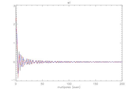
Figure 1: (left) The coefficients of the decomposition of the mask function on spherical harmonics for different galactic cuts, $\mu_{c}=10,20$ and 30 deg. (respectively black, red and blue lines). Only the non-vanishing, that is even, multipoles are plotted. (right) The ratio $w_{\ell}/w_{0}$ decreases rapidly and becomes typically smaller than 0.1% for $\ell$ larger than 20 (plain=10 deg., dot=20 deg., dash-dot=30 deg.).

III.3 Properties of the $\widetilde{a}_{\ell m}$

Whatever the choice of the mask, as long as it satisfies the properties (27), the general expression of the coefficients $\widetilde{a}_{\ell m}$ of the decomposition of $\widetilde{\Theta}$, are given by

$$\widetilde{a}_{\ell m}=f_{\rm sky}a_{\ell m}+(-1)^{m}\sqrt{2\ell+1}\sum_{{\ell_{1}}}\sqrt{\frac{2{\ell_{1}}+1}{4\pi}}a_{{\ell_{1}}m}\sum_{{\ell_{2}}\not=0}\sqrt{2{\ell_{2}}+1}\hat{w}_{\ell_{2}}\left(\begin{array}[]{ccc}{\ell_{1}}&{\ell_{2}}&\ell\\ m&0&-m\end{array}\right)\left(\begin{array}[]{ccc}{\ell_{1}}&{\ell_{2}}&\ell\\ 0&0&0\end{array}\right)$$ (31)

with $f_{\rm sky}\equiv w_{0}/\sqrt{4\pi}$ is the fraction of the sky that is covered. From this expression, we deduce that their 2-point function is given by

$$\left<\widetilde{a}_{\ell m}\widetilde{a}_{\ell^{\prime}m^{\prime}}^{*}\right>=\delta_{mm^{\prime}}\left\{C_{\ell}f_{\rm sky}^{2}\delta_{\ell\ell^{\prime}}+f_{\rm sky}\left[{\cal G}(\ell,\ell^{\prime},m)C_{\ell}+{\cal G}(\ell^{\prime},\ell,m)C_{\ell^{\prime}}\right]+\sum_{\ell_{1}}C_{{\ell_{1}}}{\cal G}({\ell_{1}},\ell,m){\cal G}({\ell_{1}},\ell^{\prime},m)\right\}$$ (32)

where the function ${\cal G}(\ell,\ell^{\prime},m)$ is defined by

$${\cal G}(\ell,\ell^{\prime},m)=(-1)^{m}\sqrt{(2\ell+1)(2\ell^{\prime}+1)}\sum_{{\ell_{2}}\not=0}\sqrt{\frac{2{\ell_{2}}+1}{4\pi}}\hat{w}_{\ell_{2}}\left(\begin{array}[]{ccc}\ell&{\ell_{2}}&\ell^{\prime}\\ m&0&-m\end{array}\right)\left(\begin{array}[]{ccc}\ell&{\ell_{2}}&\ell^{\prime}\\ 0&0&0\end{array}\right).$$ (37)

It follows from Eq. (32) that there is no $m$-coupling arising from the mask (because it has no azimuthal dependence) and we can define the correlation matrix of the masked temperature field as

$$\left<\widetilde{a}_{\ell m}\widetilde{a}_{\ell m^{\prime}}^{*}\right>\equiv\widetilde{C}_{\ell m}\delta_{mm^{\prime}}.$$ (38)

The angular power spectrum of the mask field is then defined as

$$\widetilde{C}_{\ell}=\frac{1}{2\ell+1}\sum_{m=-\ell}^{\ell}\widetilde{C}_{\ell m}$$ (39)

and is explicitly given in terms of the primordial angular power spectrum by

$$\widetilde{C}_{\ell}=C_{\ell}\left[f_{\rm sky}^{2}+2\frac{f_{\rm sky}}{2\ell+1}\sum_{m=-\ell}^{\ell}{\cal G}(\ell,\ell,m)\right]+\sum_{\ell_{1}}\frac{C_{\ell_{1}}}{2\ell+1}\sum_{m=-\ell}^{\ell}{\cal G}^{2}({\ell_{1}},\ell,m).$$ (40)

Let us now turn to the $\ell$-$(\ell+1)$ correlators. The first term in Eq. (32) vanishes. Then, one can check that ${\cal G}(\ell,\ell+1,m)$ vanishes because the triangular relation of the Wigner-$3j$ symbols implies that $\ell_{2}=\pm 1$ but for odd ${\ell_{2}}$ $\hat{w}_{\ell_{2}}$ vanish. To finish, the contribution of ${\cal G}(\ell_{1},\ell,m){\cal G}(\ell_{1},\ell+1,m)$ in the sum also vanishes because ${\ell_{2}}$ is even and the sums ${\ell_{1}}+{\ell_{2}}+\ell+1$ and ${\ell_{1}}+{\ell_{2}}+\ell$ have to be both even, which is impossible. In conclusion

$$\left<\widetilde{a}_{\ell m}\widetilde{a}_{\ell+1m^{\prime}}^{*}\right>=0.$$ (41)

As expected from our construction, the mask does not generate $\ell$-$(\ell+1)$ correlations.

To finish, let us stress that the mask will induce some $\ell$-$\ell+2$ correlations that can be characterized by introducing

$${\,{}_{2}}\widetilde{C}_{\ell m}\equiv\left<\widetilde{a}_{\ell m}\widetilde{a}_{\ell+2m}^{*}\right>,\qquad{\,{}_{2}}\widetilde{C}_{\ell}\equiv\frac{1}{2\ell+1}\sum_{m=-\ell}^{\ell}{\,{}_{2}}\widetilde{C}_{\ell m}.$$ (42)

Indeed, when $W={\rm Id}$, ${\,{}_{2}}\widetilde{C}_{\ell}=0$.

III.4 General construction

Starting from the relation (17) and the expression (26), we deduce that the two quantities defined in Eqs. (11-12) generalize to

$$D_{\ell m}^{(i)} = \sqrt{\frac{3}{4\pi}}\varepsilon_{i}^{*}\left\{(-1)^{\ell+m+1+i}\sqrt{\ell+1}\left(\begin{array}[]{ccc}\ell&1&\ell+1\\ m&i&-m-i\end{array}\right)\left[\widetilde{C}_{\ell m}+\widetilde{C}_{\ell+1m+i}\right]\right.$$ (51)

$$\qquad\qquad+(-1)^{\ell+m+i}\sqrt{\ell}\left(\begin{array}[]{ccc}\ell-1&1&\ell\\ m+i&-i&-m\end{array}\right){\,{}_{2}}\widetilde{C}_{\ell-1m+i}$$

$$\qquad\qquad\left.+(-1)^{\ell+m+i}\sqrt{\ell+2}\left(\begin{array}[]{ccc}\ell+1&1&\ell+2\\ -m-i&i&m\end{array}\right){\,{}_{2}}\widetilde{C}_{\ell m}\right\},$$

with $i=0,1$, when the mask effects are taken into account. This expression is defined for $m=-\ell\ldots\ell$ even if ${\,{}_{2}}\widetilde{C}_{\ell-1m+1}$ is not defined for $m=\ell$ and $m=\ell-1$ and ${\,{}_{2}}\widetilde{C}_{\ell-1m}$ for $m=\ell$ because the Wigner-$3j$ symbols that multiply these terms strictly vanish. From this expression, we define

$$D_{\ell}^{(i)}\equiv\frac{\sum_{m=-\ell}^{\ell}(-1)^{\ell+m+1+i}\left(\begin{array}[]{ccc}\ell&1&\ell+1\\ m&i&-m-i\end{array}\right)D^{(i)}_{\ell m}}{\sum_{m=-\ell}^{\ell}(-1)^{\ell+m+1+i}\left(\begin{array}[]{ccc}\ell&1&\ell+1\\ m&i&-m-i\end{array}\right)}.$$ (52)

Now, it can be checked, after some algebra, that

$$D_{\ell}^{(i)}=\sqrt{\frac{3}{4\pi}}\varepsilon_{i}^{*}\left[\hat{C}_{\ell}^{(i)}+2\,{{}_{2}}{\hat{C}}_{\ell}^{(i)A}+2\,{{}_{2}}{\hat{C}}_{\ell}^{(i)B}\right]+{\cal O}(\varepsilon^{2})$$ (53)

where the quantities $\hat{C}_{\ell}^{(i)}$, ${{}_{2}}{\hat{C}}_{\ell}^{(i)A}$ and ${{}_{2}}{\hat{C}}_{\ell}^{(i)B}$ have been defined by

$$\hat{C}_{\ell}^{(i)} = \frac{1}{N^{(i)}_{\ell}}\sum_{m=-\ell}^{\ell}\sqrt{\ell+1)}\left(\begin{array}[]{ccc}\ell+1&1&\ell\\ m&i&-m-i\end{array}\right)^{2}\left[\widetilde{C}_{\ell m}+\widetilde{C}_{\ell+1m+i}\right]$$ (56)

$${{}_{2}}{\hat{C}}_{\ell}^{(i)A} = -\frac{1}{N^{(i)}_{\ell}}\sum_{m=-\ell}^{\ell}\sqrt{\ell+2}\left(\begin{array}[]{ccc}\ell&1&\ell+1\\ m&i&-m-i\end{array}\right)\left(\begin{array}[]{ccc}\ell+2&1&\ell+1\\ m&i&-m-i\end{array}\right){{}_{2}}\widetilde{C}_{\ell m}$$ (61)

$${{}_{2}}{\hat{C}}_{\ell}^{(i)B} = -\frac{1}{N^{(i)}_{\ell}}\sum_{m=-\ell}^{\ell}\sqrt{\ell}\left(\begin{array}[]{ccc}\ell&1&\ell+1\\ m&i&-m-i\end{array}\right)\left(\begin{array}[]{ccc}\ell-1&1&\ell\\ m+i&-i&-m\end{array}\right){{}_{2}}\widetilde{C}_{\ell m}$$ (66)

with the coefficients $N^{(i)}_{\ell}$ given by

$$N^{(i)}_{\ell}=\sum_{m=-\ell}^{\ell}(-1)^{\ell+m+i}\left(\begin{array}[]{ccc}\ell&1&\ell+1\\ m&i&-m-i\end{array}\right).$$ (67)

It follows from these results that we can consider the estimator

$$E_{\ell}^{(i)} = \frac{1}{N^{(i)}_{\ell}}\sum_{m=-\ell}^{\ell}\left(\begin{array}[]{ccc}\ell&1&\ell+1\\ m&i&-m-i\end{array}\right)(-1)^{\ell+m+i}\,a_{\ell m}^{\rm obs}a_{\ell+1m+i}^{{\rm obs}*}$$ (70)

that satisfies by construction

$$\left<E^{(i)}_{\ell}\right>=D_{\ell}^{(i)}.$$ (71)

We will apply this estimator to the WMAP data in the following sections.

IV Data analysis

The proposed estimators have been implemented numerically, using the Healpix package for the pixelization and the fast spherical harmonics transforms, and applied to the co-added data of the WMAP V and W bands (resp. ${\rm 70\,GHz}$ and ${\rm 90\,GHz}$) where most of the signal is of cosmological origin. We implemented the estimators as described by equations (53) to (70).

The quantities $\hat{C}_{\ell}^{(i)}$, ${}_{2}\hat{C}_{\ell}^{(i)A}$ and ${}_{2}\hat{C}_{\ell}^{(i)B}$ have been computed using the best fit LCDM theoretical power spectrum of the WMAP data [28], and were not computed on the data itself to avoid ratios of random variables. To assess the statistical significance of the measured values of $\varepsilon_{i}$, we made $1000$ simulations of WMAP data in each of the V and W bands according to a sky model with no modulation.

The results of the analysis of the V and W bands are summarized on Figs. 2 to 5. Fig. 2 depicts the measurement of $D_{\ell}$ on the W band. We sum this measurement of two bands of $\ell$ (respectively 20-100 and 100-300) and compare with 1000 simulated WMAP data. We perform the same tests on the V band (Fig. 4 and 5). The apparent detection in the V band without clear counterpart in the W band suggest a non cosmological contamination. Determining its origin requires to performed more tests.

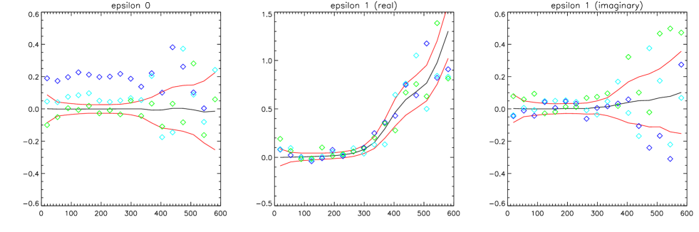
Figure 2: $D_{\ell}$ measured on the WMAP data (W band) [green triangles]. Blue triangles are the measurements on a simulated map with ${\varepsilon_{0}}=0.2$ and the red lines are $1\sigma$ error bars.

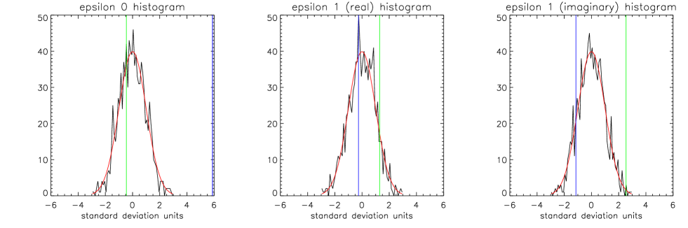
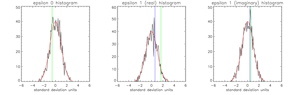
Figure 3: Comparison of 1000 simulations with the WMAP data. We use the W band and sum the multipole between $\ell=20$ and $\ell=100$ (top panel) and between $\ell=100$ and $\ell=300$ (bottom panel). The color code is identical to the one of Fig. 2 that is the green line correspond to the measurement on the WMAP data and the blue line the measurement on a simulation.

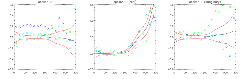
Figure 4: $D_{\ell}$ measured on the WMAP data (V band) [green traingles]. Blue triangles are the measurements on a simulated map with ${\varepsilon_{0}}=0.2$ and the red lines are $1\sigma$ error bars.

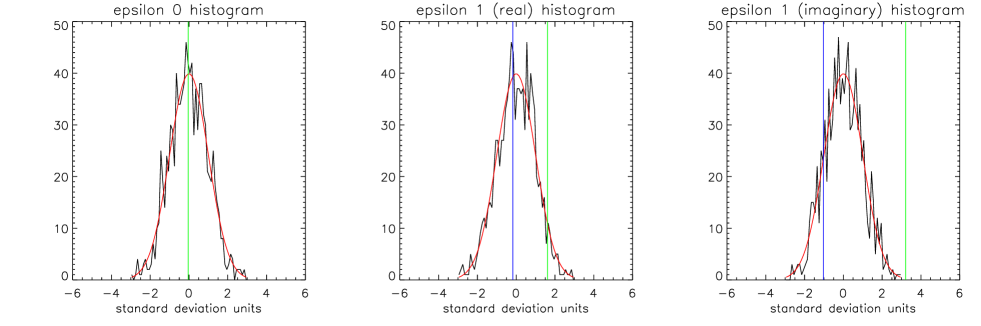
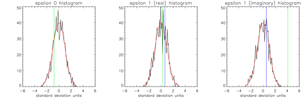
Figure 5: Comparison of 1000 simulations with the WMAP data. We use the V band and sum the multipole between $\ell=20$ and $\ell=100$ (top panel) and between $\ell=100$ and $\ell=300$ (bottom panel).

This contamination can be a priori from two possible sources, Galactic or extragalactic. To check if the correlations detected in the V band are of Galactic origin, we apply the same estimator to the half sum and half difference of the V and W bands, that is

$$S=\frac{W+V}{2},\qquad D=\frac{W-V}{2}$$ (72)

and repeat the whole procedure on 1000 simulation in each case, where the simulations contain only CMB and noise according to the WMAP specifications. The advantage of the half difference of the bands is that it should (up to calibration errors) eliminate the CMB signal completely at large scales, hence eliminate the main source of variance at these same scales, where the Galactic signals are expected to dominate. Indeed, the power spectra of Galactic emissions usually scale as $C_{\ell}\propto\ell^{-\alpha}$, with $2\leq\alpha\leq 3$ (see e.g. Ref. [29]). The half sum results, summarized in table I, are in between those of the V and W bands, which is coherent with the assumption of the detection being caused by a foreground source of electromagnetic spectrum different from the CMB fluctuations.

More importantly, the half difference results do not show a strong correlation detection at large angular scales, in contradiction with the assumption of the Galactic foreground contamination being the source of the detected correlations in the V band.

However, this half difference test does not work that well if the source contaminants are of extragalactic origin, since the power spectra of extragalactic foregrounds resemble that of the noise. In this case, the contamination is expected to increase with increasing multipole number, which seems to be the case for the V band (see Figs. 4 and 5).

The difficulty of extragalactic point sources contamination is that these sources (quasars and active radio-galaxies) are distributed more or less uniformly across the sky, which renders their masking by an azimuthally symmetric sky cut impossible. However, the WMAP team provides with their data sets “taylor cuts” that blank out the resolved point sources of largest flux. Of course, the dipolar modulation estimators designed in the preceding sections do not apply stricto sensu to these arbitrary masks, but one can hope, given the small fraction of sky removed at high latitude, that the broken symmetry of the mask will be a small perturbation in the computation of the $\varepsilon$’s, so that the estimators keep their general validity, up to a possible small bias (see Fig. 8 for a comparison of the coefficients $w_{\ell}$ of the two masks).

This assumption can be checked on a simulated sky with a known dipolar modulation, where a WMAP V-band noise is added to the signal, together with the taylor mask. We chose the most conservative mask provided by the WMAP team (kp0), and applied it to a simulated sky of known modulation ($\varepsilon_{0}=0.2$) as described above, together with the V-band data. The results are shown in figures 6 and  7. Again, the estimators have been applied to $1000$ simulations of the V band with no dipolar modulation, with the same kp0 mask applied, to estimate the statistics of the V-band data results.

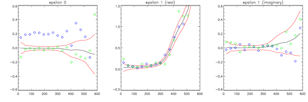
Figure 6: $D_{\ell}$ measured on the WMAP data (V band) [green triangles], using the taylor mask kp0 to blank the main point sources. Blue triangles are the measurements on a simulated map with ${\varepsilon_{0}}=0.2$ and the red lines are $1\sigma$ error bars.

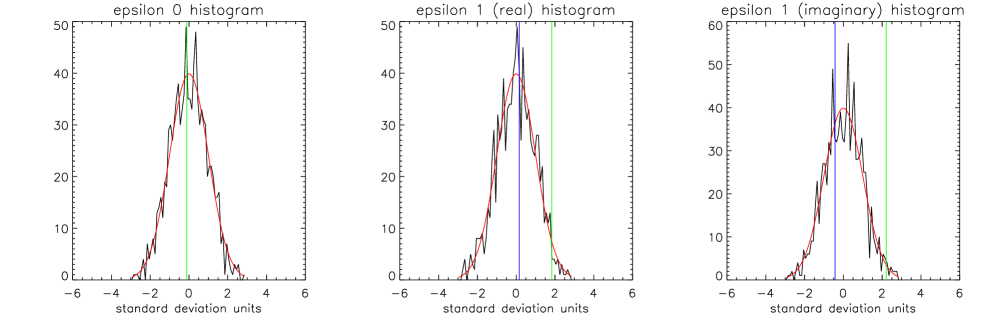
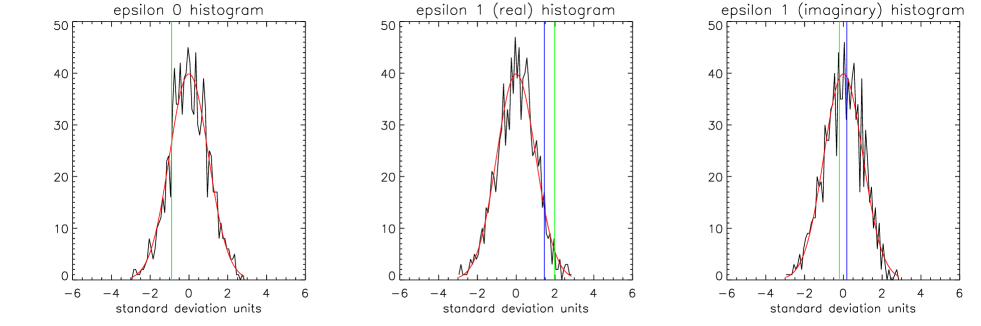
Figure 7: Comparison of 1000 simulations with the WMAP data. We use the V band and sum the multipole between $\ell=20$ and $\ell=100$ (top panel) and between $\ell=100$ and $\ell=300$ (bottom panel) using the taylor mask kp0 to blank the main point sources.

Several observations can be made at this point. First, comparing these results with those obtained in the V-band, but with the azimuthally symmetric $20^{\circ}$ cut (figure 4), one can check that the estimators give very compatible results for the simulated dipolar modulation (blue squares). This comforts our assumption that changing the cut sky to the kp0 mask is a small perturbation for the modulation estimators.

Secondly, comparing the same figures but this time looking at the data (green squares), one can see that in the case of the $20^{\circ}$ cut there is a large trend at high $\ell$’s in $\varepsilon_{1}$ that disappears when the kp0 cut is used. This is confirmed by the results of table 1 where one can check that the tentative detections of in the V band using the simple cut become statistically insignificant when using the kp0 cut.

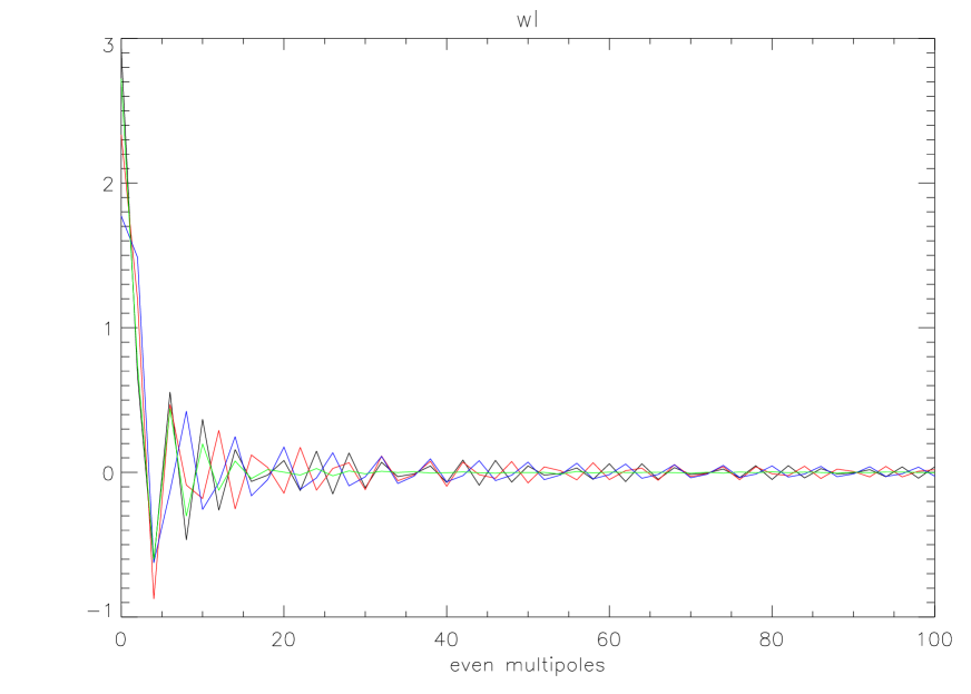
Figure 8: The coefficients of of the decomposition of the mask function on spherical harmonics for different galactic $\mu_{c}=10,20$ and 30 deg. (respectively black, red and blue lines) compared with the ones of the kp0 mask (green).

V Discussion and conclusions

In this article we have proposed an estimator designed to detect a possible modulation of the CMB temperature field, or equivalently $\Delta\ell=1$ correlations. The effects of cutting part of the sky were discussed in details and we applied this estimator to the V and W bands of the WMAP data.

The results of our analysis are summarized in table 1 which gives the amplitude of the modulation coefficients on the WMAP data and a corresponding test case with ${\varepsilon_{0}}=0.2$, $\hbox{Re}(\varepsilon_{1})=\hbox{Im}(\varepsilon_{1})=0$. All values are given in standard deviation units, estimated on 1000 (signal+noise) simulations in each case, with no modulations.

While the V band seems to exhibit a marginal detection, further tests such as the study of the half sum and difference of the two bands and the effect of point sources have led us to conclude that this detection should be inferred to the effect of point sources contamination. In this analysis we have used the kp0 mask which does not satisfied the symmetries of the mask required for our estimator to be unbiased. Nevertheless, our estimator seems to be well suited for the analysis, even with the kp0 mask.

To back up this interpretation we have performed two last tests. First we added to a simulated CMB map without modulation and with noise the 208 sources resolved by the WMAP experiment and then smoothed with the correct beam. Second we added to the same simulation the 700 circular region that are cut in the analysis of the V band in the WMAP analysis. Both simulations, while analyzed as the previous data with an azimuthal mask of 20 deg., exhibit an excess of signal for ${\varepsilon_{0}}$ and $\hbox{Im}(\varepsilon_{1})$ in the same range of multipoles than obtained on the analysis of the V and W bands (Figs. 2 and 4). Interestingly, the signal of $\hbox{Re}(\varepsilon_{1})$ is not affected and is identical to the one of Figs. 2 and 4. Indeed, the signals have not exactly the same amplitude as the ones obtained from the analysis of the V band but they exhibit the same trend on the the same scales. Also, it has to be stressed that with a cut of 20 deg. the Large Magellannic Cloud (galactic latitude of 20 deg. and more and longitude of 0 deg.) and a part of the H2 Ophucius region should contribute and that we have not included them in the simulations. This could have enhance the signal.

In conclusion, the set of analysis performed in our study tend to show that the $\Delta\ell=1$ correlations that appeared in the analysis of the V and W bands of the WMAP data are due to foreground contaminations and most likely by point sources. The direction of the detected modulation will, in that interpretation, characterize the anisotropy of the distribution of these sources.

	${\varepsilon_{0}}$		Re($\varepsilon$)		Im($\varepsilon$)
	data	test	data	test	data	test
W (20-100)	-0.45	5.87	1.30	-0.26	2.54	-1.14
W (100-300)	-0.60	16.9	1.65	0.61	0.59	0.41
V (20-100)	-0.04	6.00	1.61	-0.17	3.21	-1.03
V (100-300)	-0.81	17.9	0.25	0.65	4.10	0.54
V-kP0 20-100)	-0.11	6.12	1.83	0.16	2.20	-0.42
V-kp0 (100-300)	-0.89	17.4	1.98	1.45	-0.22	0.18
S (20-100)	-0.24	6.71	1.52	0.40	2.85	-0.31
S (100-300)	-0.64	19.3	1.15	0.57	2.16	1.35
D (20-100)	-0.58	-0.74	-2.10	-1.49	3.73	-0.70
D (100-300)	-0.98	0.93	-0.44	0.69	2.67	-0.54

Table 1: Summary of the data analysis performed in this article. It concerns the two bands V and W, their half sum (S) and half difference (D). The band V has been analyzed with two masks to emphasize the effect of the point sources on the result.

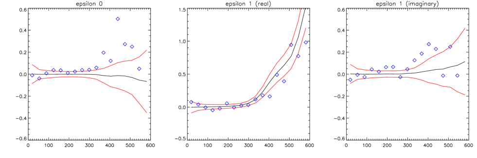
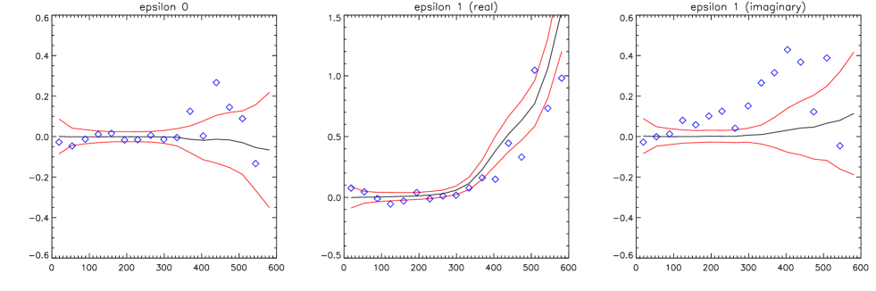
Figure 9: The analysis of the simulated maps in which (top) the 208 resolved sources of the WMAP catalog have been added and (bottom) where the 700 point sources (resolved and unresolved) of the V band have been added. In both cases, the signal of $\hbox{Re}(\varepsilon_{1}$ is not affected while the signal of ${\varepsilon_{0}}$ and $\hbox{Im}(\varepsilon_{1})$ exhibit patterns that are similar to the ones obtained in our analysis of the V and W band on the same angular scales.

Acknowledgements: Some of the results of this article have been derived using the HEALPix package [30]. We thank Y. Mellier and R. Stompor for discussions.

Appendix A Integrals over spherical harmonics

We have evaluated integrals over $n$ spherical harmonics (see Ref. [31]). When $n=1$ or 2, these integrals are trivial

$$\int{\rm d}^{2}\,{\vec{\gamma}}Y_{\ell m} = \sqrt{4\pi}\delta_{\ell 0}\delta_{m0}$$ (73)

$$\int{\rm d}^{2}\,{\vec{\gamma}}Y_{{\ell_{1}}{m_{1}}}Y_{{\ell_{2}}{m_{2}}}^{*} = \delta_{{\ell_{1}}{\ell_{2}}}\delta_{{m_{1}}{m_{2}}}.$$ (74)

To go further, one solution is to use the decomposition of the product of 2 spherical harmonics as

$$Y_{{\ell_{1}}{m_{1}}}({\vec{\gamma}})Y_{{\ell_{2}}{m_{2}}}({\vec{\gamma}})=\sum_{LM}\sqrt{\frac{(2{\ell_{1}}+1)(2{\ell_{2}}+1}{4\pi(2L+1)}}C_{{\ell_{1}}0{\ell_{2}}0}^{L0}C_{{\ell_{1}}{m_{1}}{\ell_{2}}{m_{2}}}^{LM}Y_{LM}({\vec{\gamma}})$$ (75)

where the $C_{{\ell_{1}}{m_{1}}{\ell_{2}}{m_{2}}}^{LM}$ are the Clebsch-Gordan coefficients that can be expressed in terms of Wigner $3j$ symbols as

$$C_{{\ell_{1}}{m_{1}}{\ell_{2}}{m_{2}}}^{LM}=(-1)^{{\ell_{1}}-{\ell_{2}}+M}\sqrt{2L+1}\left(\begin{array}[]{ccc}{\ell_{1}}&{\ell_{2}}&L\\ {m_{1}}&{m_{2}}&-M\end{array}\right)$$ (76)

It is easy to generalize Eq. (75) to a product of $n$ spherical harmonics

$$Y_{{\ell_{1}}{m_{1}}}\ldots Y_{\ell_{n}m_{n}}=\sum_{L_{n},M_{n}}\left[\sqrt{\frac{4\pi}{2L_{n}+1}}\sum_{L_{1}\ldots L_{n-1},M_{1}\ldots M_{n-1}}\prod_{i=1}^{n}\left(\sqrt{\frac{2\ell_{i}+1}{4\pi}}C_{L_{i-1}0\ell_{i}0}^{L_{i}0}C_{L_{i-1}M_{i-1}\ell_{i}m_{i}}^{L_{i}M_{i}}\right)\right]Y_{L_{n}M_{n}}.$$ (77)

We deduce, using Eq. (77) and the integral (74) that

$$\int{\rm d}^{2}{\vec{\gamma}}Y_{{\ell_{1}}{m_{1}}}Y_{{\ell_{2}}{m_{2}}}Y_{\ell_{3}m_{3}}^{*} = \sqrt{\frac{(2{\ell_{1}}+1)(2{\ell_{2}}+1)}{4\pi(2\ell_{3}+1)}}C_{{\ell_{1}}0{\ell_{2}}0}^{\ell_{3}0}C_{{\ell_{1}}{m_{1}}{\ell_{2}}{m_{2}}}^{\ell_{3}m_{3}}$$ (78)

$$\int{\rm d}^{2}{\vec{\gamma}}Y_{{\ell_{1}}{m_{1}}}Y_{{\ell_{2}}{m_{2}}}Y_{\ell_{3}m_{3}}Y_{\ell_{4}m_{4}}^{*} = \sum_{L,M}\sqrt{\frac{(2{\ell_{1}}+1)(2{\ell_{2}}+1)(2\ell_{3}+1)}{(4\pi)^{2}(2\ell_{4}+1)}}C_{{\ell_{1}}0{\ell_{2}}0}^{L0}C_{L0\ell_{3}0}^{\ell_{4}0}C_{{\ell_{1}}{m_{1}}{\ell_{2}}{m_{2}}}^{LM}C_{LM\ell_{3}m_{3}}^{\ell_{4}m_{4}}.$$ (79)

References

- [1] C.L. Bennett et al., Astrophys. J. Suppl. 148 (2003) 1.
- [2] D.N. Spergel et al., Astrophys. J. Suppl. 148 (2003) 175.
- [3] H.V. Peiris et al., Astrophys. J. Suppl. 148 (2003) 213.
- [4] M. Tegmark, A. de Oliveira-Costa, and A. Hamilton, Phys. Rev. D 68 (2003) 123503.
- [5] J.-P. Uzan, U. Kirchner, and G.F.R. Ellis, Month. Not. R. Astron. Soc. 343 (2003) L95.
- [6] G. Efstathiou, Month. Not. R. Astron. Soc. 343 (2003) L95.
- [7] A. Slosar, U. Seljak, and A. Makarov, [arXiv:astro-ph/0403073].
- [8] A. de Oliveira-Costa, M. Tegmark, M. Zaldarriaga, and A. Hamilton, Phys. Rev. D 69 (3004) 63516.
- [9] D. Schwarz et al., [arXiv:astro-ph/0403353].
- [10] E. Komatsu et al., Astrophys. J. Suppl. 148 (2003) 119.
- [11] A. Haijan and T. Souradeep, Astrophys. J. 597 (2003) L5.
- [12] C.J. Copi, D. Huterer, and G. Starkman, [arXiv:astro-ph/0310511].
- [13] F.K. Hansen, P. Cabella, D. Marinucci, and N. Vittorio, [arXiv:astro-ph/0402396].
- [14] H.K. Eriksen, D.I. Novikov, P.B. Lilje, A.J. Banday, and K.M. Gorski, [arXiv:astro-ph/0401276].
- [15] H.K. Eriksen, F.K. Hansen, A.J. Banday, K.M. Gorski, and P.B. Lilje, [arXiv:astro-ph/0307507].
- [16] C.-G. Park, Month. Not. R. Astron. Soc. 349 (2004) 313.
- [17] D.L. Larson and B. Wandelt, [arXiv:astro-ph/0404037].
- [18] L.-Y. Chiang, P.D. Naselsky, O. Verkhodanov, and M. Way, Astrophys. J. Lett 590 (2003) 65.
- [19] K. Land and J. Magueijo, [arXiv:astro-ph/0405519].
- [20] A. Slosar and U. Seljak, [arXiv:astro-ph/0404567].
- [21] F. Bernardeau and J.-P. Uzan, Phys. Rev. D 66 (2002) 103506.
- [22] F. Bernardeau and J.-P. Uzan, Phys. Rev. D 67 (2003) 121301(R).
- [23] F. Bernardeau and J.-P. Uzan, Phys. Rev. D (in press), [arXiv:astro-ph/0311421].
- [24] F. Bernardeau, T. Brunier and J.-P. Uzan, (in preparation).
-
[25]
A. Riazuelo, J.-P. Uzan, R. Lehoucq, J. Weeks,
Phys. Rev. D 69 (2004) 103514;
A. Riazuelo, J.-P. Uzan, R. Lehoucq, J. Weeks, and J.-P. Luminet, Phys. Rev. D 69 (2004) 103518;
J.-P. Uzan and A. Riazuelo, C.R. Acad. Sciences (Paris) 4 (2003) 945;
J.-P. Uzan, A. Riazuelo, R. Lehoucq, and J. Weeks, Phys. Rev. D 69 (2004) 043003,
J.-P. Luminet, J. Weeks, A. Riazuelo, R. Lehoucq, and J.-P. Uzan, Nature (London) 425 (2003) 593. -
[26]
R. Durrer, T. Kahniashvili, and T.A. Yates,
Phys. Rev D 58 (1998) 123004;
A. Mack, T. Kahniashvili, and A. Kosowsky, Phys. Rev. D 65 (2002) 123004;
G. Chen, P. Mukherjee, T. Kahniashvili, B. Ratra, and Y. Wang, [arXiv:astro-ph/0403695];
P.D. Naselsky, L.-Y. Chiang, P. Olesen, and O. Verkhodanov, [arXiv:astro-ph/0405181]. - [27] E. Hivon et al., Astrophys. J. 567 (2002) 2.
- [28] L. Verde et al., Astrophys. J. Suppl. 148 (2003) 195.
- [29] F.R. Bouchet and Gispert, New Astron. 4 (1999) 443.
- [30] K.M. Górski, E. Hivon, and B.D. Wandelt, in Proceedings of the MPA/ESO Cosmology Conference ”Evolution of large-scale structure”, Eds. A.J. Banday et al. (PrintPartners Ipskamp, NL, 1999), pp. 37-42, [arXiv:astro-ph/9812350].
- [31] D.A. Varshalovich, A.N. Moskalev, and V.K. Khersonskii, “Quantum theory of angular momentum”, (World Scientific, Singapore, 1988).