The Cosmic Microwave Background and Its Polarization

Abstract

The DASI discovery of CMB polarization, confirmed by WMAP, has opened a new chapter in cosmology. Most of the useful information about inflationary gravitational waves and reionization is on large angular scales where Galactic foreground contamination is the worst. The goal of the present review is to provide the state-of-the-art of the CMB polarization from a practical point of view, connecting real-world data to physical models. We present the physics of this polarized phenomena and illustrate how it depends of various cosmological parameters for standard adiabatic models. We also present all observational constraints to date and discuss how much we have learned about polarized foregrounds so far from the CMB studies. Finally, we comment on future prospects for the measurement of CMB polarization.

University of Pennsylvania, Dept. of Physics & Astronomy, Philadelphia, 19104 PA, USA

1. Introduction

The recent discovery of cosmic microwave background (CMB) polarization by the DASI (Degree Angular Scale Interferometer) experiment kovac02 , confirmed by the WMAP (Wilkinson Anisotropy Probe) satellite kogut03 , has opened a new chapter in cosmology – see Figure 2. Although CMB polarization on degree scales and below can sharpen cosmological constraints and provide an important cross-check on our basic assumptions about the behavior of fluctuations in the universe ZSS97 ; Eisenstein98 , the potential for the most dramatic improvements lies on the largest angular scales where it provides a unique probe of the reionization epoch and primordial gravitational waves.

CMB polarization is produced via Thomson scattering which occurs either at decoupling or during reionization. The level of this polarization is linked to the local quadrupole anisotropy of the incident radiation on the scattering electrons, and it is expected to be of order 1%-10% of the amplitude of the temperature anisotropies depending on the angular scale – see ZH95 ; HW97 and references therein.

The goal of the present review is to survey the state-of-the-art of CMB polarization from a practical point of view, connecting real-world data to physical models. In $Section~{}\ref{physics}$ and $Section~{}\ref{theo}$, we summarize the physics of CMB polarization and illustrate how it depends on various cosmological parameters for standard adiabatic models. In $Section~{}\ref{measurements}$, we present all observational constraints to date. In $Section~{}\ref{foregrounds}$, we discuss how such measurements can be compromised by the Galactic foregrounds. Finally, we conclude in $Section~{}\ref{conclusions}$ with comments on future prospects for the measurement of CMB polarization.

2. How does CMB polarization form?

At times before decoupling, the universe was hot enough that protons and electrons existed freely in a plasma. Through Thomson scattering, they kept tightly coupled, i.e., they were in thermal equilibrium at a common temperature. As a consequence of this tight coupling epoch, the radiation field could only possess a monopole (given by the plasma’s temperature) and a dipole (described as a Doppler shift due to the peculiar velocities in the fluid). Any higher moment was damped away due to scattering, and no net polarization could be produced (i.e., the radiation field was unpolarized).

As the temperature of the universe drooped (below 3,000K), protons and electrons started to recombine into neutral hydrogen. The mean free path grown rapidly and the eletrons began to see local quadrupoles within the plasma. At this point, Thomsom scattering started to produce polarized light. By the time almost all free electrons were used up to produce neutral hydrogen, Thomson scattering ceased for lack of scatterers, and the radiation was said to decouple. From that point on, this radiation, known as the CMB, propagated freely until the universe reionized around $z\approx 17$.

3. Polarization phenomenology

Whereas most astronomers use the Stokes parameters $Q$ and $U$ to describe polarization measurements, the CMB community uses two scalar fields $E$ and $B$ that are independent of how the coordinate system is oriented, and are related to the tensor field $(Q,U)$ by a non–local transformation K97 ; ZS97 ; Z98 . Scalar CMB fluctuations have been shown to generate only curl-free $E$-modes, whereas gravity waves, CMB lensing and foregrounds generate both $E$ and a pure curl component called $B$-modes.

3.1. The six power spectra

Since CMB measurements can be decomposed into three maps ($T$,$E$,$B$), where $T$ denotes the unpolarized component, there are a total of 6 angular power spectra that can be measured. Expanding the $T$, $E$ and $B$ maps in spherical harmonics with coefficients $a_{\l m}^{T}$, $a_{\l m}^{E}$ and $a_{\l m}^{B}$, these 6 spectra are defined by

$$C_{\l}^{T}=\langle a_{\l m}^{T*}a_{\l m}^{T}\rangle,C_{\l}^{E}=\langle a_{\l m}^{E*}a_{\l m}^{E}\rangle,C_{\l}^{B}=\langle a_{\l m}^{B*}a_{\l m}^{B}\rangle,C_{\l}^{X}=\langle a_{\l m}^{T*}a_{\l m}^{E}\rangle,$$

$$C_{\l}^{Y}=\langle a_{\l m}^{T*}a_{\l m}^{B}\rangle,C_{\l}^{Z}=\langle a_{\l m}^{E*}a_{\l m}^{B}\rangle,$$

corresponding to $TT$, $EE$, $BB$, $TE$, $TB$ and $EB$ correlations, respectively TC01 . By parity, $C_{\l}^{Y}=C_{\l}^{Z}=0$ for scalar CMB fluctuations, but it is nonetheless worthwhile to measure these power spectra as probes of both exotic physics KK99 ; XK99 ; Kamionkowski00 and foreground contamination angel_polar . $C_{\l}^{B}=0$ for scalar CMB fluctuations to first order in perturbation theory K97 ; ZS97 ; Z98 ; HuWhite97 — secondary effects such as gravitational lensing can create $B$ polarization even if there are only density perturbations present ZSLENS . In the absence of reionization, $C_{\l}^{E}$ is typically a couple of orders of magnitude below $C_{\l}^{T}$ on small scales and approaches zero on the very largest scales.

3.2. Covariance versus correlation

The cross-power spectrum $C_{\l}^{X}$ is not well suited for the usual logarithmic power spectrum plot, since it is negative for about half of all $\l$-values angel_pique . Sometimes, a theoretically more convenient quantity is the dimensionless correlation coefficient $r^{X}_{\l}\equiv{C_{\l}^{X}\over(C_{\l}^{T}C_{\l}^{E})^{1/2}}$, plotted on a linear scale in Figure 1 (Right, lower panel), since the Schwarz inequality restricts it to lie in the range $-1\leq r^{X}_{\l}\leq 1$. From here on we use $r_{\l}$ as shorthand for $r^{X}_{\l}$. For more details about $r_{\l}$ and how it depends on cosmological parameters, see section II.b in angel_pique .

3.3. Cosmological parameter dependence of polarization spectra

A detailed review of how CMB polarization reflects underlying physical processes in given in HW97 . In this subsection, we briefly review this topic from a more phenomenological point of view (see also Jaffe00 ), focusing on how different cosmological parameters affect various features in the $E$, $B$ and $X$ power spectra. For more details, the reader is referred to the polarization movies at www.hep.upenn.edu/$\sim$angelica/polarization.html.

Let us consider adiabatic inflationary models specified by the following 10 parameters: the reionization optical depth $\tau$, the primordial amplitudes $A_{s}$, $A_{t}$ and tilts $n_{s}$, $n_{t}$ of scalar and tensor fluctuations, and five parameters specifying the cosmic matter budget. The various contributions $\Omega_{i}$ to critical density are for curvature $\Omega_{\rm k}$, vacuum energy $\Omega_{\Lambda}$, cold dark matter $\Omega_{\rm cdm}$, hot dark matter (neutrinos) $\Omega_{\nu}$ and baryons $\Omega_{\rm b}$. The quantities $\omega_{\rm b}\equiv h^{2}\Omega_{\rm b}$ and $\omega_{\rm dm}\equiv h^{2}\Omega_{\rm dm}$ correspond to the physical densities of baryons and total (cold + hot) dark matter ($\Omega_{\rm dm}\equiv\Omega_{\rm cdm}+\Omega_{\nu}$), and $f_{\nu}\equiv\Omega_{\nu}/\Omega_{\rm dm}$ is the fraction of the dark matter that is hot. The baseline values of the parameters here and in the movies are for the concordance model of X01 ; spergel03 ; sdsswmap03 . All power spectra were computed with the CMBfast software SZ96 .

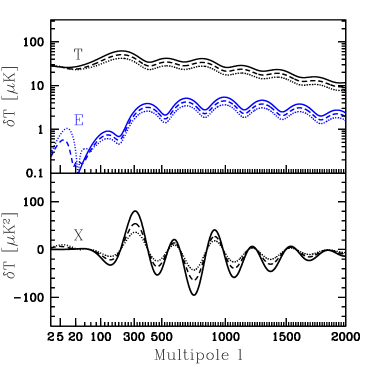
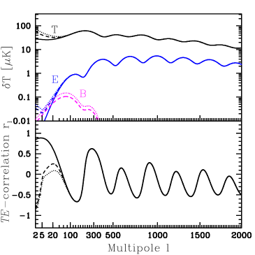
Figure 1.: Left: How the reionization optical depth $\tau$ affects the $T$ and $E$ power spectra (top panel) and the $X$ power spectra (lower panel). Solid, dashed and dotted curves correspond to for $\tau$=0, 0.2 and 0.4, respectively. Right: How the gravity wave amplitude $A_{t}$ affects the $T$, $E$ and $B$ power spectra (top panel) and the correlation coefficient $r_{\l}$ (lower panel). Solid, dashed and dotted curves correspond to for $A_{t}$=0, 0.2 and 0.4, respectively.

Polarized versus unpolarized:

If recombination were instantaneous (with the radiation field locally isotropic), there would be no polarization at all.

Both the $E$ and the $T$ power spectra carry information about the $z\mathrel{\hbox to0.0pt{\lower 3.0pt\hbox{$\mathchar 536\relax$}\hss}\raise 2.0pt\hbox{$\mathchar 318\relax$}}10^{3}$ pre-recombination epoch in the form of acoustic oscillations. From a practical point of view, there are two obvious differences between the $E$ and $T$ power spectra as illustrated by Figure 1:

• The $E$ power is smaller since the polarization percentage is small, making measurements more challenging. This is because polarization is only generated when locally anisotropic radiation scatters off of free electrons, and this only occurs during the brief period when recombination is taking place: before recombination, radiation is quite isotropic and after recombination there is almost no scattering.

• Aside from reionization effects, the $E$ power approaches zero on scales much larger than those of the first acoustic peak. This is because the polarization anisotropies are only generated on scales of order the mean free path at recombination and below.

As detailed below, changing the cosmological parameters affects the polarized and unpolarized power spectra rather similarly except for the cases of reionization and gravity waves. Another interesting difference between the power spectra of the temperature and polarization is that they exhibit peaks which are approximately a half-cycle out of phase – see Figure 1. As described above, as recombination proceeds, the eletrons begin to see radiation Doppler-shifted by the velocity fields in the plasma and scattering leads to polarization. Since $E$-mode polarization arises from velocities, when the fluid velocity drops to zero, the amplitude of the polarization will fall to a minimum at the compression or expansion maxima of the density mode. Similarly, the amplitude of the polarization will be highest at the density nulls, when the fluid velocity reaches a maximum. The $X$ spectrum, on the other hand, has a more complex behavior with the sign of the correlation depending on whether the amplitude of the mode was increasing or decreasing at the time of decoupling.

Reionization

Reionization at redshift $z_{*}$ introduces a new scale $\l_{*}\sim 20(z_{*}/10)^{1/2}$ corresponding to the horizon size at the time. Primary (from $z\mathrel{\hbox to0.0pt{\lower 3.0pt\hbox{$\mathchar 536\relax$}\hss}\raise 2.0pt\hbox{$\mathchar 318\relax$}}1000$) fluctuations $\delta T_{\l}$ on scales $\l\gg\l_{*}$ get suppressed by a factor $e^{\tau}$ and new series of peaks are generated starting at the scale $\l_{*}$. Figure 1 (Left, top panel) illustrates that although these new peaks are almost undetectable in $T$, drowning in sample variance from the unpolarized Sachs-Wolfe effect, they are clearly visible in $E$ and $X$ since the Sachs-Wolfe nuisance is unpolarized and absent. The models in Figure 1 have abrupt reionization giving $\tau\propto z_{*}^{3/2}$, so higher $z_{*}$ is seen to shift the new peaks both up and to the right. For more details about CMB polarization and reionization see Z97 ; Hu00 .

Primordial perturbations:

As seen in Figure 1 (Right, top panel), gravity waves (a.k.a. tensor fluctuations) contribute only to fairly large angular scales, producing $E$ and $B$-polarization. Just as for the reionization case, unpolarized fluctuations are also produced but are difficult to detect since they get swamped by the Sachs-Wolfe effect. As has been frequently pointed out in the literature, no other physical effects (except CMB lensing and foregrounds) should produce $B$-polarization, potentially making this a smoking gun signal of gravity waves. Gravitational waves created by inflation would produce $B$-modes in the CMB. Because such waves decay after entering the horizon, the spectrum of such $B$-mode signal should peak at large angular scales, with an amplitude that is tied to the inflationary energy scale.

Adding a small gravity wave component is seen to suppress the correlation $r_{\l}$ in Figure 1 (Right, lower panel), since this component is uncorrelated with the dominant signal that was there previously. Indeed, this large-scale correlation suppression may prove to be a smoking gun signature of gravity waves that is easier to observe in practice than the often-discussed $B$-signal Knox ; Kesden . This $TE$-correlation suppression comes mainly from $E$, not $T$: since the tensor polarization has a redder slope than the scalar polarization, it can dominate $E$ at low $\l$ even while remaining subdominant in $T$. Foreground and lensing signals would need to be accurately quantified for this test, since they would also reduce the correlation.

The amplitudes $A_{s}$, $A_{t}$ and tilts $n_{s}$, $n_{t}$ of primordial scalar and tensor fluctuations simply change the amplitudes and slopes of the various power spectra: B is controlled by $(A_{t},n_{t})$ alone, whereas $T$ and $E$ are affected by $(A_{s},n_{s})$ and $(A_{t},n_{t})$ in combination. Note that if there are no gravity waves ($A_{t}=0$), then these amplitudes and tilts cancel out, leaving the correlation spectrum $r_{\l}$ independent of both $A_{s}$ and (apart from aliasing effects) $n_{s}$.

4. Polarization measurements and upper limits

Since the detection of the CMB by Penzias and Wilson in 1965 PW65 , experimentalists have been checking (among other things) if the CMB is also polarized. A fact unknown to many is that the first constrain on CMB polarization can also be credited to Penzias and Wilson. In their groundbreaking paper, they stated that the new radiation they had detected was not only isotropic but also unpolarized within the limits of their observations. Over the next 37 years, dedicated polarimeters were constructed to set much more stringent upper limits on the CMB, culminating in 2002 with its detection by the DASI experiment and later re-confirmed by WMAP. These are the only CMB polarization detections we have so far.

DASI was a ground-based experiment located near the Amundsen-Scott South Pole Research Station. Observations in all four Stokes parameters were obtained within two $3\hbox{${}^{\circ}$}.4$ FWHM fields separated by one hour in RA. The $E$-polarization mode was detected at 4.9$\sigma$, while the $X$ cross-polarization mode was detected at 2$\sigma$ kovac02 . WMAP is an ongoing space mission that produces full sky $I$, $Q$ and $U$ CMB maps at 5 frequencies between 23 and 94 GHz and angular resolutions from 0^∘.82 to 0^∘.21, probing 2 $\mathrel{\hbox to0.0pt{\lower 3.0pt\hbox{$\mathchar 536\relax$}\hss}\raise 2.0pt\hbox{$\mathchar 316\relax$}}\l\mathrel{\hbox to0.0pt{\lower 3.0pt\hbox{$\mathchar 536\relax$}\hss}\raise 2.0pt\hbox{$\mathchar 316\relax$}}$ 600 bennett03 . The first year data have resulted in confirmation of the large scale $X$ cross-correlation at the 10$\sigma$ level, an extraordinary direct evidence of significant reionization at higher redshifts. The data agrees with the concordance $\Lambda$CDM model, with the best-fit value $\tau$=0.17$\pm$0.04 at 68% confidence. This implies z_r=17$\pm$3 kogut03 ; page03 .

We next briefly review the history of CMB polarization measurements (subdividing them by angular scale). For comparison, we show all measurements and limits on CMB polarization to date in Figure 2, and a list with some of the ongoing and future CMB polarization experiments in Table 1

Table 1.: Ongoing & Future CMB Polarization Experiments

Experiment FWHM $\nu$ Receiver^a Sensitivity Area Site-yr^b Ref. [GHz] [$\mu$K$\sqrt{s}$] CAPMAP 4’ 30,90 HEMT 1000 $\delta>$89^∘ NJ barkats03 CBI 45’ 30 HEMT 40$(\hbox{${}^{\circ}$})^{2}$ Atacama pearson03 DASI 26-36 2 $3\hbox{${}^{\circ}$}.4$ Fields SP kovac02 KuPID 0^∘.2 15 370 $\delta>$87^∘ NJ gundersen03 Polatron 2.5’ 100 B 8000 Ring/NCP OVRO philhour01 AMiBA 1’-19’ 90 HEMT 7$\mu$k/hr Fields:100(’)² HI-04 lo03 BICEP 1^∘,0^∘.7 100,150 B 280 -5$\hbox{${}^{\circ}$}>\delta>$-25^∘ SP-05 keating03 Polarbear 90-350 B CA-05 tran03 QUEST 4’ 100,150 B 300 SP-05 church03 SPT B SP-06 carlstrom03 Archeops 12’ 143-545 B 200 30$\%$ of Sky hamilton04 B2K 9.5’,6.5’,7’ 145,245,345 B 160,290,660 1284$(\hbox{${}^{\circ}$})^{2}$ SP montroy03 MAXIPOL 10’ 140,420 B 130 2^∘ ”bow tie” NM johnson03 WMAP 0^∘.82-0^∘.21 23-94 All Sky L2 bennett03 PlanckLFI 33’,24’,14’ 30,44,70 HEMT 7.7^∗,10^∗,18^∗ All Sky L2-07 lawrence03 PlanckHFI 9.2’,7.1’ 100,143 B …,11^∗ All Sky L2-07 lamarre03 5’ 217,353 B 27^∗,81^∗ 5’ 545,857 B SPOrt 7^∘ 22,32,60,90 HEMT 1000 80$\%$ of Sky Sp.Stat. carretti02

^aB = Bolometer.
^bSP = South Pole; L2 = An orbit about the 2^nd Lagrange point of the Sun-Earth system; Sp.Stat = Space Station.
^∗Sensitivity values are in $\mu$K averaged over the sky for 12 months of integration.

4.1. Large angular scale (2 $\mathrel{\hbox to0.0pt{\lower 3.0pt\hbox{$\mathchar 536\relax$}\hss}\raise 2.0pt\hbox{$\mathchar 316\relax$}}\l\mathrel{\hbox to0.0pt{\lower 3.0pt\hbox{$\mathchar 536\relax$}\hss}\raise 2.0pt\hbox{$\mathchar 316\relax$}}$ 30)

Since the pioneering work of Caderni C78 , Nanos N79 , Lubin & Smoot LS79 ; LS81 ; L83 and Sironi S98 , years passed until polarized detector technology achieved sensitivity levels that were below the levels of the CMB temperature anisotropy. The first of such achievements came on large scales with the POLAR (Polarization Observations of Large Angular Regions) experiment keating01 . POLAR was a ground-based experiment that operated near Madison, Wisconsin. It used a simple drift-scan strategy, with a 7^∘ FWHM beam at 30 GHz, and simultaneously observed the Stokes parameters $Q$ and $U$ in a ring of declination $\delta=43\hbox{${}^{\circ}$}$. The POLAR experiment provided an upper limit on $E$- and $B$-modes of 10$\mu$K at 95% confidence for the multipole range of 2 $\mathrel{\hbox to0.0pt{\lower 3.0pt\hbox{$\mathchar 536\relax$}\hss}\raise 2.0pt\hbox{$\mathchar 316\relax$}}\l\mathrel{\hbox to0.0pt{\lower 3.0pt\hbox{$\mathchar 536\relax$}\hss}\raise 2.0pt\hbox{$\mathchar 316\relax$}}$ 20 keating01 , and an upper limit on the $X$-mode of 11.1$\mu$K at 95% confidence level over a similar multipole range from its cross-correlation with the COBE/DMR map angel_polar . POLAR was later reconfigured to become the COMPASS experiment at intermediate angular scales farese03 . To date, the only CMB polarization detection on large angular scales is the cross-correlation detected by WMAP.

4.2. Intermediate angular scale (50 $\mathrel{\hbox to0.0pt{\lower 3.0pt\hbox{$\mathchar 536\relax$}\hss}\raise 2.0pt\hbox{$\mathchar 316\relax$}}\l\mathrel{\hbox to0.0pt{\lower 3.0pt\hbox{$\mathchar 536\relax$}\hss}\raise 2.0pt\hbox{$\mathchar 316\relax$}}$ 1000)

The first upper limits at intermediate angular scales came from the works of P88 ; F93 ; W93 ; T99 . However, the best upper limit over this same angular range (before its detection by DASI) was set more than ten years later by PIQUE (Princeton I, Q and U Experiment), see H00 . PIQUE was a CMB polarization experiment on the roof of the physics building at Princeton University. It used a single 90 GHz correlation polarimeter with FWHM angular resolution of 0^∘.235, and observed $Q$ and $U$ in a ring of radius of 1^∘ around the NCP (North Celestial Pole). PIQUE provided an upper limit on $E$- and $B$-modes of 8.4$\mu$K at 95% confidence over the multipole range 59 $\mathrel{\hbox to0.0pt{\lower 3.0pt\hbox{$\mathchar 536\relax$}\hss}\raise 2.0pt\hbox{$\mathchar 316\relax$}}\l\mathrel{\hbox to0.0pt{\lower 3.0pt\hbox{$\mathchar 536\relax$}\hss}\raise 2.0pt\hbox{$\mathchar 316\relax$}}$ 334 H02 , and an upper limit on the $X$-mode of 17.3$\mu$K at 95% confidence over a similar multipole range from its cross-correlation with the SK (Saskatoon) map angel_pique . PIQUE has been reconfigured to become the CAPMAP (Cosmic Anisotropy Polarization Mapper) experiment barkats03 , which plans to observe a cap of 1^∘ radius around the NCP with 4’ FWHM at 30 and 90 GHz. CAPMAP also shares observing location and technology with KuPID (Ku-band Polarization Identifier) gundersen03 . KuPID will measure $Q$ and $U$ Stokes parameters in a region near the NCP ($\delta>87\hbox{${}^{\circ}$}$) at 12-18 GHz. The primary research objectives of KuPID include surveying the polarized component of Galactic synchrotron, characterizing Foreground-X, measuring CMB polarization (if foregrounds are not too limiting), and performing follow-up measurements of interesting regions identified by WMAP.

Two other ground-based experiments are being developed to be deployed at the South Pole by 2005: BICEP and QUEST. The BICEP (Background Imaging of Cosmic Extragalactic Polarization) experiment keating03 will observe the South Celestial Pole at 100 and 150 GHz, probing 10 $\mathrel{\hbox to0.0pt{\lower 3.0pt\hbox{$\mathchar 536\relax$}\hss}\raise 2.0pt\hbox{$\mathchar 316\relax$}}\l\mathrel{\hbox to0.0pt{\lower 3.0pt\hbox{$\mathchar 536\relax$}\hss}\raise 2.0pt\hbox{$\mathchar 316\relax$}}$ 200. QUEST (Q and U Extragalactic Survey Telescope) is expected to be mounted on the DASI teslescope church03 . It will also observe the CMB at the same frequency range of BICEP, but with a higher angular resolution of FWHM=4’.

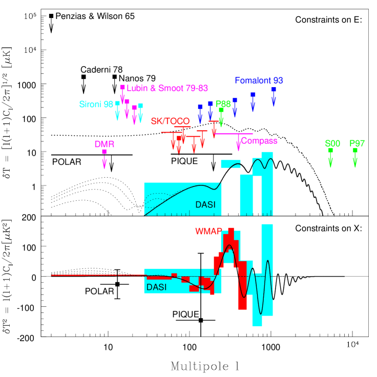
Figure 2.: Summary of constraints on polarization so far. From top to bottom, the three curves show the concordance model predictions for $C_{\l}^{T}$, $C_{\l}^{E}$ and $C_{\l}^{X}$, respectively. Four reionization models with $\tau$=0.1, 0.2, 0.3 and 0.4 are also plotted (left dotted lines from bottom to top in both plots). The limits for $E$ are shown in the upper panel: Penzias & Wilson 65 PW65 , Caderni 78 C78 , Nanos 79 N79 , Lubin & Smoot 79-83 LS79 ; LS81 ; L83 (magenta squares), Sironi 98 S98 (cyan squares), Fomalont 93 F93 , P88 P88 , SK/TOCO W93 ; T99 (square: SK), S00 S00 , P97 P97 , DMR smootDMR , POLAR keating01 and PIQUE H02 , COMPASS farese03 . The limits for $X$ are shown in the lower panel: POLAR angel_polar and PIQUE angel_pique . The shaded cyan and red regions are the DASI kovac02 and WMAP page03 results, respectively.

There are also CMB polarization measurements at intermediate scales done from balloons. The current generation of balloon-borne experiments include BOOMERanG montroy03 , MAXIPOL johnson03 and Archeops benoit03 . Polarized BOOMERanG (also known as B2K) made a successful long-duration balloon flight over Antarctica during the Austral summer of 2003. It operated at 145, 245 and 345 GHz with a 10’ beam, mapping two regions in the sky: the first centered at (RA,DEC) $\approx 75,-45$ with an area of 1161 deg² and another close to the Galactic Plane with an area of 393 deg². MAXIPOL had successful flight form Ft. Sumner (NM) in May, 2003. It operated at 140 and 420 GHz with an angular resolution of 10’. Finally, the Archeops experiment also made a successful balloon flight in 2002 and produced maps with measurements of the Galactic dust polarization benoit03 , which we discuss in more details in the next section.

4.3. Small angular scales ($\l>$ 1000)

CMB polarization measurements have also been pursued on smaller scales, resulting only in upper limits P97 ; S00 . Today, small-scale ground-based experiments, such as AMiBA (Array for Microwave Background Anisotropy; lo03 ), SPT (South Pole Telescope; carlstrom03 ) and ACT (Atacama Cosmology Telescope; kosowsky03 ), are working on filling this gap. AMiBA will operate around 90 GHz and observe the four Stokes parameters. It is to be deployed on Mauna Kea, Hawaii, with initial observations targeting $E$-modes by 2004. SPT is expected to be deployed by 2006 and ACT is planned to be deployed in Chile, which could also be equipped with a polarimeter.

Also on the works are the next generation of CMB satellites. The Planck Surveyor lawrence03 ; lamarre03 , which is a dedicated CMB satellite, is scheduled to launch in 2007. It will measure the entire sky in 9 frequencies between 30 and 857 GHz with an angular resolution that can probe 2$\mathrel{\hbox to0.0pt{\lower 3.0pt\hbox{$\mathchar 536\relax$}\hss}\raise 2.0pt\hbox{$\mathchar 316\relax$}}\l\mathrel{\hbox to0.0pt{\lower 3.0pt\hbox{$\mathchar 536\relax$}\hss}\raise 2.0pt\hbox{$\mathchar 316\relax$}}$2000. However, the most ambitious plan on the horizon is for a dedicated CMB polarization satellite to conduct a search (only foreground limited) for signatures of inflationary gravitational waves in the CMB, or to measure its $B$-modes. This is the goal of the Inflation Probe in NASA’s “Beyond Einstein program”.

5. Polarized foregrounds

Understanding the physical origin of Galactic microwave emission is interesting for two reasons: to determine the fundamental properties of the Galactic components, and to refine the modeling of foreground emission in CMB experiments. At microwave frequencies, three physical mechanisms are known to cause foreground contamination: synchrotron and free-free emission (both major contaminants at frequencies below 60 GHz), and dust emission (which is a major contaminant above 100 GHz). When coming from extragalactic objects, this radiation is usually referred to as point source contamination and affects mainly small angular scales. When coming from the Milky Way, this diffuse Galactic emission fluctuates mainly on large angular scales. Except for free-free emission, all the above mechanisms are known to emit polarized radiation.

Most of the useful information about inflationary gravitational waves and reionization is on large angular scales where Galactic foreground contamination is the worst, so a key challenge is to model, quantify and remove polarized foregrounds. Unfortunately, these large scales are also the ones where polarized foreground contamination is likely to be most severe, both because of the red power spectra of diffuse Galactic synchrotron and dust emission and because they require using a large fraction of the sky, including less clean patches. A key challenge in the CMB polarization endeavor will therefore be modeling, quantifying and removing large-scale polarized Galactic foregrounds.

Studies of CMB polarization must also deal with a second type of foreground, related to gravitational lensing. Since the deflection of light rays by weak gravitational lensing can rotate polarization vectors, CMB $E$-modes can be partially converted into $B$-modes with a power that is proportional to the lensing signal (see, e.g., ZSLENS ). Fortunately, such a $B$-component can be at least partially reconstructed and removed from the CMB using the fact that it introduces non-Gaussianities in the data – see, e.g., smith03 and references therein.

5.1. Galactic synchrotron emission

Unfortunately, we still know basically nothing about the polarized contribution of the Galactic synchrotron component at CMB frequencies (see, e.g., allforegpars and references therein), since it has only been measured at lower frequencies and extrapolation is complicated by Faraday Rotation. This is in stark contrast to the CMB itself, where the expected polarized power spectra and their dependence on cosmological parameters has been computed from first principles to high accuracy K97 ; ZS97 ; Z98 ; HuWhite97 .

There is a recent study of the Leiden surveys BS76 ; S84 that try to shed some light on the properties of the Galactic polarized synchrotron emission at the CMB frequencies angel_polar . This study observed that the synchrotron $E$- and $B$-contributions are equal to within 10% from 408 to 820 MHz, with a hint of $E$-domination at higher frequencies. One interpretation of this result is that $E>B$ at CMB frequencies but that Faraday Rotation mixes the two at low frequencies. It was also found that Faraday Rotation & Depolarization effects depend not only on frequency but also on angular scale, i.e., they are important at low frequencies ($\nu\mathrel{\hbox to0.0pt{\lower 3.0pt\hbox{$\mathchar 536\relax$}\hss}\raise 2.0pt\hbox{$\mathchar 316\relax$}}10$ GHz) and on large angular scales. Finally, combining the POLAR and radio frequency results from the Leiden surveys, and using the fact that the $E$-polarization of the abundant Haslam signal in the POLAR region is not detected at 30 GHz, suggests that the synchrotron polarization percentage at CMB frequencies is rather low.

In the near future, the best measurement of large-scale Galactic polarized synchrotron will come from the WMAP satellite. In WMAP’s frequency range (22-90 GHz), the study of its $E$ maps will allow better quantification of synchrotron, and certainly confirm (or refute) the findings described above.

5.2. Galactic dust emission

Polarized microwave emission from dust is an important foreground that may strongly contaminate polarized CMB studies unless accounted for. At higher frequencies ($\mathrel{\hbox to0.0pt{\lower 3.0pt\hbox{$\mathchar 536\relax$}\hss}\raise 2.0pt\hbox{$\mathchar 318\relax$}}$ 100 GHz) the main contamination comes from vibrational dust emission, while at lower frequencies (15 $\mathrel{\hbox to0.0pt{\lower 3.0pt\hbox{$\mathchar 536\relax$}\hss}\raise 2.0pt\hbox{$\mathchar 316\relax$}}\nu\mathrel{\hbox to0.0pt{\lower 3.0pt\hbox{$\mathchar 536\relax$}\hss}\raise 2.0pt\hbox{$\mathchar 316\relax$}}$ 60 GHz) it may come from another dust population composed basically of small grains that emit radiation via rotational rather than vibrational excitations DL98 .

This small grain component, nicknamed Foreground-X tenerife2 , is spatially correlated with the 100 $\mu$m dust emission but with a spectrum that rises towards lower frequencies, subsequently flattening and turning down somewhere around 15 GHz. Although there is plenty of observational evidence in favor of its existency (see tenerife3 and references therein), there is no spatial template for this component. If Foreground-X is due to spinning dust particles, the amount of polarization of this component is marginal for $\nu\mathrel{\hbox to0.0pt{\lower 3.0pt\hbox{$\mathchar 536\relax$}\hss}\raise 2.0pt\hbox{$\mathchar 318\relax$}}$ 35 GHz. However, if Foreground-X emission is due to the magneto-dipole mechanism the polarization can be substantial – see LF03 for details.

For the case of polarized vibrational dust emission, little is known, and experiments such as Archeops and B2K are probably our best short-term hope for trying to understand its behavior at microwave frequencies. For instance, the Archeops experiment detected polarized emission by dust at 353 GHz benoit03 . They find that the diffuse emission from the Galactic plane is 4-5% polarized, and its orientation is mostly perpendicular to the plane. There is evidence for a powerful grain alignment mechanism throughout the interstellar medium.

6. Conclusions: what to expect for the future?

CMB polarization is likely to be a goldmine of cosmological information, allowing to improve measurements of many cosmological parameters and numerous important cross-checks and tests of the underlying theory. For some of the future goals, such as to detect gravity waves through CMB polarization, we will need to develop new polarized detector technology and better understand the polarized foregrounds (Galactic and extragalactic). In fact, our ability to measure cosmological parameters using the CMB will only be as good as our understanding of the microwave foregrounds. To do a good job removing foregrounds, we need to understand their frequency and scale dependence, frequency coherence, and better characterize their non-Gaussian behavior.

Acknowledgements: The author wish to thank Max Tegmark for proof-reading the manuscript. Support was provided by the NASA grant NAG5-11099.

References

- (1) (1) J. Kovac et al., Nature 420, 772 (2002).
- (2) (2) A. Kogut et al., ApJS 148, 161 (2003).
- (3) (3) M. Zaldarriaga, D. N. Spergel, and U. Seljak, ApJ 488, 1 (1997).
- (4) (4) D. J. Eisenstein, W. Hu, and M. Tegmark, ApJ 518, 2 (1999).
- (5) (5) M. Zaldarriaga and D. Harari, Phys.Rev. D 52, 2 (1995).
- (6) (6) W. Hu and M. White, New Astron. 2, 323 (1997).
- (7) (7) A. Kamionkowski, A. Kosowsky, and A. Stebbins, Phys.Rev. D 55, 7368 (1997).
- (8) (8) M. Zaldarriaga and U. Seljak, Phys.Rev. D 55, 1830 (1997).
- (9) (9) M. Zaldarriaga, ApJ 503, 1 (1998).
- (10) (10) M. Tegmark and A. de Oliveira-Costa, Phys.Rev. D 64, 063001 (2001).
- (11) (11) M. Kamionkowski, and A. Kosowsky, Ann.Rev. Nucl. Part. Sci. 49, 77 (1999).
- (12) (12) X. Chen, and M. Kamionkowski, Phys.Rev. D 60, 104036 (1999).
- (13) (13) M. Kamionkowski , and A. H. Jaffe, Int.J.Mod.Phys. A 16, 116 (2001).
- (14) (14) A. de Oliveira-Costa et al., Phys.Rev. D 68, 083003 (2003).
- (15) (15) W. Hu , and M. White, Phys.Rev. D 56, 596 (1997).
- (16) (16) M. Zaldarriaga, and U. Seljak, Phys.Rev. D 580, 3003 (1998).
- (17) (17) A. de Oliveira-Costa et al., Phys.Rev. D 67, 023003 (2003).
- (18) (18) A. H. Jaffe, M. Kamionkowski, and L. Wang, Phys.Rev. D 61, 083501 (2000).
- (19) (19) X. Wang, M. Tegmark, and M. Zaldarriaga, Phys.Rev. D 65, 123001 (2002).
- (20) (20) D. Spergel et al., ApJS 148, 175 (2003).
- (21) (21) M. Tegmark et al., Phys.Rev. D 69, 103501 (2004).
- (22) (22) U. Seljak, and M. Zaldarriaga, ApJ 469, 437 (1996).
- (23) (23) M. Zaldarriaga, Phys.Rev. D 55, 1822 (1997).
- (24) (24) W. Hu, ApJ 529, 12 (2000).
- (25) (25) L. Knox, and Y. Song, Phys.Rev. Lett. 89, 011303 (2002).
- (26) (26) M. Kesden, A. Cooray, and M. Kamionkowski, Phys.Rev. Lett. 89, 011304 (2002).
- (27) (27) A. A. Penzias, and R. W. Wilson, ApJ 142, 419 (1965).
- (28) (28) C. L. Bennett et al., astro-ph/0302207 (2003).
- (29) (29) L. Page et al., astro-ph/0302220 (2003).
- (30) (30) N. Caderni, Phys.Rev. D 17, 1908 (1978).
- (31) (31) G. Nanos, ApJ 232, 341 (1979).
- (32) (32) P. M. Lubin, and G. F. Smoot, Phys.Rev. Lett. 42(2), 129 (1979).
- (33) (33) P. M. Lubin, and G. F. Smoot, ApJ 245, 1 (1981).
- (34) (34) P. M. LubinP. Melese, and G. F. Smoot, ApJ 273, 51 (1983).
- (35) (35) G. Sironi et al., New Astronomy 3, 1 (1998).
- (36) (36) B. Keating et al., ApJ 560, 1 (2001).
- (37) (37) P. C. Farese, astro-ph/0308309 (2003).
- (38) (38) R. B. Partridge, J. Nawakowski, and H. M. Martin, Nature 311, 146 (1988).
- (39) (39) E. B. Fomalont et al., ApJ 404, 8 (1993).
- (40) (40) E. J. Wollack et al., ApJ 419, 49 (1993).
- (41) (41) E. Torbet et al., ApJ 521, 79 (1999).
- (42) (42) M. Hedman et al., ApJL 548, 111 (2001).
- (43) (43) M. Hedman et al., astro-ph/0204438 (2002).
- (44) (44) D. Barkats, New Astron. Rev. 47, 1077 (2003).
- (45) (45) J. O. Gundersen, New Astron. Rev. 47, 1097 (2003).
- (46) (46) B. Keating et al., Proc. of SPIE 4843, 284 (2003).
- (47) (47) S. Church et al., New Astron. Rev. 47, 1083 (2003).
- (48) (48) T. Montroy et al., New Astron. Rev. 47, 1067 (2003).
- (49) (49) B. R. Johnson et al., New Astron. Rev. 47, 1047 (2003).
- (50) (50) A. Benoit et al., A&A 399, L19 (2003).
- (51) (51) R. B. Partridge et al., ApJ 483, 38 (1997).
- (52) (52) R. Subrahmanyan et al., MNRAS 315, 808 (2000).
- (53) (53) K. Lo Y et al., astro-ph/0012282 (2000).
- (54) (54) J. E. Carlstrom et al., New Astron. Rev. 47, 953 (2003).
- (55) (55) A. kosowsky, New Astron. Rev. 47, 939 (2003).
- (56) (56) C. R. Lawrence, New Astron. Rev. 47, 1017 (2003).
- (57) (57) J. M. Lamarre et al., New Astron. Rev. 47, 1025 (2003).
- (58) (58) T. J. Pearson et al., ApJ 591, 556 (2003).
- (59) (59) B. J. Philhour et al., astro-ph/0106543 (2001).
- (60) (60) H. T. Tran, New Astron. Rev. 47, 1091 (2003).
- (61) (61) J. C. Hamilton et al., Comptes Rendus Physique 4, 853 (2003).
- (62) (62) E. Carretti et al., astro-ph/0212067 (2002).
- (63) (63) G. F. Smoot, astro-ph/9902027 (1999).
- (64) (64) K. M. Smith et al., astro-ph/0402442 (2004).
- (65) (65) C. Baccigalupi, New Astron. Rev. 47, 1127 (2003).
- (66) (66) W. N. Brouw and T. A. T Spoelstra, A&AS 26, 129 (1976).
- (67) (67) T. A. T Spoelstra, A&A 135, 238 (1984).
- (68) (68) B. Draine and A. Lazarian, ApJ 494, L19 (1998).
- (69) (69) A. de Oliveira-Costa et al., ApJ 530, 133 (2002).
- (70) (70) A. de Oliveira-Costa et al., ApJ 606, L89 (2004).
- (71) (71) A. Lazarian and D. Finkbeiner, New Astron. Rev. 47, 1107 (2003).