Automated classification of variable stars for ASAS 1-2 data

Abstract

With the advent of surveys generating multi-epoch photometry and the discovery of large numbers of variable stars, the classification of these stars has to be automatic. We have developed such a classification procedure for about 1700 stars from the variable star catalogue of ASAS 1-2 (All Sky Automated Survey, Pojmański 2000) by selecting the periodic ones and by applying an unsupervised Bayesian classifier using parameters obtained through a Fourier decomposition of the light curve. For irregular light curves we used the period and moments of the magnitude distribution for the classification. In the case of ASAS 1-2, 83% of variable objects are red giants. A general relation between the period and amplitude is found for a large fraction of those stars. The selection led to 302 periodic and 1429 semi-periodic stars which are classified in 6 major groups: eclipsing binaries, “sinusoidal curves”, Cepheids, small amplitude red variables, SR and Mira stars. The type classification error level is estimated to be about 7%.

1 Introduction

The knowledge of the bright sky variability is relatively poor. Bohdan Paczyński (2001) denounces this situation vigorously, “I think this ignorance is inexcusable and embarrassing to the astronomical community”. Yet, at magnitude 12, it is estimated that $90\%$ of the variables are unknown (Paczyński 2000).

In recent years, only the hipparcos satellite has done a multi-epoch photometric all-sky survey with an associated analysis aimed at systematically detecting variability. This survey has a mean of 110 measurements per star over 3.3 years. It goes down to V magnitude 7.3/9.0 depending on the colour of the star and its ecliptic latitude $\beta$. The result of this analysis for the main mission is published in volumes 11 and 12 of ESA (1997) (see also the flags H6, H49 to H53 of the main catalogue) and concerns 11562 variable stars that comprise about 10% of all catalogue entries. hipparcos enables the description of the behaviour of individual stars by giving mean color and magnitude, parallax, period, amplitude and epoch of the minimum or maximum light, but also for the stellar variability across the HR-diagram (Eyer & Grenon 1997) to be described globally. It is worth noting that the data classification in the different variable types was “manual” and incomplete. The tycho photometric data, a deeper survey, caused more problems in its analysis and gave somewhat disappointing results even after efforts to censor poor quality data points (Piquard et al. 2001).

There are photometric optical surveys which have specific goals, like OGLE, EROS, MACHO for detecting microlensing events, ROTSE and LOTIS for detecting gamma ray bursts. We don’t discuss those here and refer to Paczyński (2000). They were exploited for other purposes and global analyses have been done (Belokurov et al. 2003) or are underway (Woźniak P. et al. 2001).

There are many ways to conduct a survey since several competing parameters cannot all be maximized. Four primary questions are in competition: how deep, how frequently sampled, how wide, and how precise is a survey? Consequently, different astronomical subjects/objects will be explored/discovered depending on these choices.

It is important to consider this work in view of the general research trend. With surveys from the ground and from space going wider and deeper, the number of objects is increasing dramatically and the handling of data is becoming more difficult. With exponential data growth, there is a clear need for automated algorithms.

We are analysing here the ASAS survey data obtained during its test implementation (phase 1 and 2). ASAS is described in the next section. An extraction of the variable objects was done by Pojmański (2000) and we address here the question of classification of the stars of this selection. The number of objects that are considered is about 3900 variable objects, among them about 400 periodic variable objects (Pojmański 2000).

Pojmański (2002, 2003, 2004) has continued to develop ASAS, and presented an analysis of the third phase of ASAS. About 1.3/3.2 million stars brighter than $V=15$ were measured, 3126/10453 variable stars were extracted and classified as eclipsing (1046/1718), regular pulsating (778/731), Mira (132/849) and “other” (1170/7155), mostly SR, IR and LPV stars (the numbers refers to the year up to 2003/2004). The regular pulsating stars have been separated into $\delta$ Scuti stars, RRab and RRc stars, $\delta$ Cep stars (fundamental and first overtone pulsators). Pojmański’s classification methods differ from the method presented here. In his article of 2003, he used carefully selected two-dimensional projections of the Fourier coefficient space where the separation of variable types are pre-analysed and well distinguishable. This method was used by Ruciński (1993) to distinguish between contact binaries and detached ones. In Pojmański’s study of 2004, he added 2MASS photometry, using two additional parametric planes ($H-K$,$\log P$) and ($H-K$,$J-H$).

The methodology presented here is divided in three main objectives: 1) to search for periodicity, 2) to model the light curve and characterize the data by a set of parameters and to remove dubious cases, 3) to determine the variability types.

2 Data Description

ASAS (All Sky Automated Survey) is a photometric survey. Its goal is to regularly monitor the sky so as to detect any variable phenomenon. In its testbed, during the years 1997-2000, ASAS 1-2 repeatedly measured 50 fields (2x3 deg² each) and obtained photometry for about 140’000 stars in I-band with a 135 mm photolens and a 768x512 pixel CCD camera. Among the 140’000 observed stars, a set of 3890 variable objects was extracted by Pojmański (2000).

The limiting magnitude is about $I=13$ and saturation occurs for stars brighter than $I=7$. The precision of the measurements is 0.01 at 8 mag and degrades to 0.07 at 12. Those estimates were derived from the difference of successive measurements (the underlying assumption being that the variability is negligible for short time scales, see Eyer & Genton 1999). The quoted individual photometric errors are not always fully consistent with our estimates.

The dates are given in truncated Heliocentric Julian dates HJD-2450000. The time sampling and number of measurements are quite diverse. There is a large gap between 585 HJD-2450000 and 1020 HJD-2450000 which was caused by a flood in the shelter containing the telescope and the control apparatus. The histogram of the number of measurements per star is given in Fig. 1 and the histogram of time differences between successive observations in Fig. 2.

For our analysis, extreme values, which were more than 4 times the dispersion distant from the mean, were removed. Different fields had different time coverage and time span. This data heterogeneity complicates the analysis. Fig. 3 shows the time difference between the last and first epoch for each star. Since large gaps might cause problems in the analysis, only observations after 1020 HJD-2450000 were considered. However, the data before 585 HJD-2450000 were used to verify shorter periods.

3 Period search

The data were processed through the Lomb (1986) period search algorithm, which is equivalent to adjusting the parameters of a sinusoidal curve. We used the algorithm given by Press et al. (1992), in its fast version called “fasper”. The algorithm has two parameters which fix the resolution in frequency and the highest frequency searched. The first, ofac, was set to 6 while the second, hifac, was changed according to the properties of the light curve and of the sampling. In fasper, the highest frequency searched is computed given the time intervals, the number of data points and the ad hoc factor multiple (hifac) of Nyquist frequency as defined by Press et al. (1992). This factor is needed since short periods can be detected even if the data has large time gaps between measurements (see Eyer & Bartholdi 1999). We did not use a constant hifac parameter, since in certain cases (large amplitude variables) it is unnecessary to search for high frequencies. On the other hand, for short time variability very high frequencies can be found.

We computed $\sigma_{N}$, the dispersion of the difference of measurements separated by a small time interval (less than 1.5 days), and divided it by the dispersion of the signal. If this ratio is small ($<0.55$), we used hifac such that the highest frequency is equal to 0.5 1/day, if it is between 0.55 and 0.66 we used $hifac=9$, and if above 0.66 we fixed hifac so that the highest frequency is equal to 17 1/day. This was found to be a better compromise than using a single value for hifac. Long time scale and large amplitude variable stars can show a variety of irregular behaviours and trends, and therefore are prone to aliasing. The determination of the highest frequency to be searched was limited to 17 1/day. This limit was determined for the shortest pulsators which have high amplitudes ($>0.05$ ) using the $\delta$ Scuti star catalogue of Rodriguez et al. (2000). The choice of $\delta$ Scuti stars is motivated by the fact that they have the shortest periods among the high amplitude periodic variable stars. Furthermore, there is a large number of known candidates allowing statistical conclusions to be drawn. Only a small fraction of those stars would be overlooked if we take the limit at 17 1/day.

The frequency of the highest peak in the Lomb periodogram is selected as being the main frequency of the signal. The amplitude $A$ of a sinusoidal signal with a standard deviation of $\sigma$ and nmes measurements is related to the power $P$ by the relation $A=\sqrt{4\,\sigma\,P/\mbox{nmes}}$.

4 Fourier series

A Fourier series with $n(\geq 2)$ harmonics is fitted to the data,

$$S(t)=\sum_{i=1}^{n}A_{i}\sin(2\pi\nu t)+B_{i}\cos(2\pi\nu t),$$

$\nu$ being the frequency, $t$ the time. The parameters

$$R_{21}=\sqrt{\frac{A_{2}^{2}+B_{2}^{2}}{A_{1}^{2}+B_{1}^{2}}}$$

and

$$\phi_{21}=\arctan{(-A_{2}/B_{2})}-2\arctan{(-A_{1}/B_{1})}$$

are computed. We linearize the equations with respect to the frequency, and search for the least square fit iteratively. The initial frequency is the one obtained with the Lomb algorithm.

The determination of the number of harmonics was done iteratively. Initially, the number of harmonics is fixed at 2, so that $R_{21}$ and $\phi_{21}$ are always defined. The procedure is then to loop and stop at a maximum of 6 harmonics. We determine a first solution for a certain number of harmonics, then we increase by one the number of harmonics and recompute a second solution. We perform a Fisher test comparing the two models (Lupton 1993). If there is a significant reduction of the $\chi^{2}$ by adding a harmonic we repeat the procedure by adding one more and if not we keep the first model. The majority of stars (58%) have a solution with two harmonics, then 18, 11, 7, 6 % have solutions with 3, 4, 5, 6 harmonics respectively.

4.1 Estimation of the Error on the Period

The general trend is that the error on the period is function of the square of the period. However, peculiarities in the light curve such as sharp features, like rising branches in Cepheids, may fix the period more precisely.

The method used for estimating the error on periods is the same as the one used for the hipparcos catalogue (ESA 1997) in the case of the Geneva solutions (Eyer 1998). We use the estimation of the error on the frequency given by the least square fit of a linearized Fourier series. Schwarzenberg-Czerny (1991) proposed an estimate for the error on the period by taking into account the correlation of the residuals. Such correction is not implemented here.

5 Cleaning the sample

To select a “well behaved” data set, we used the following criteria:

• The stars with less than 40 measurements are discarded.

• We defined a reduced time span: The total observational time span where the three largest gaps are subtracted. We retained periods which are smaller than the reduced time span divided by 1.2. It was found empirically that many short frequencies are spurious. Such a criterion may exclude true Long Period Variable stars with poorly covered light curve.

• We rejected objects with a skewness on the I magnitude larger than $-1$ (rejecting time series containing bright outliers like flares, cosmic rays).

• We selected objects which have a mean I magnitude smaller than $12.65$.

• A parabolic curve was fitted to the data, then subtracted from it and the Lomb algorithm was recomputed on the resulting data under the same conditions as the initial trial described in section 3. We present the diagram of the initial period and the period found after having subtracted that parabolic fit in Fig. 4. We notice that one-day and half-day spurious periods are present. We also notice that there are periods which are not stable. We selected the objects which have a difference of the two determined frequencies that just allows a confusion between neighbouring peaks in the Fourier spectrum.

• Periods near the aliases of one day and half a day were removed.

These criteria were established mostly empirically after the samples rejected were studied in a detailed manner to avoid rejecting valuable objects.

6 Autoclass

Humans by nature have trouble visualizing multidimensional data sets especially those with more than 3 dimensions. More than 3 attributes are needed to classify the light curves by the proposed Fourier decomposition. Furthermore, the variable star population is diverse. Some groups have very well defined characteristics, others have overlapping properties. Some classes are divided almost arbitrarily into different groups although they represent a continuum. For example, as defined in the GCVS (Kholopov et al. 1985), Mira stars have a peak to peak amplitude in V larger than 2.5 mag. An unsupervised program might give some indications for better divisions. Another advantage of such an unsupervised algorithm is that it can point out new classes of objects.

Autoclass (Cheeseman, Stutz 1996) is a Bayesian classifier. The algorithm looks for the number of classes and the classification which is most probable, given the observed data. The method was successfully applied to several astronomical sets: iras sources (Goebel et al. 1989), asteroids (Ivezic et al. 2001), and hipparcos data (Eyer unpublished).

The method is not fully automated since there is an interactive part (the class models have to be specified), but the method takes the data in its totality and proposes a broad classification. As pointed out by the authors of Autoclass, this interactivity is necessary.

Another useful aspect of the Bayesian classifier is that it computes a class membership probability. Therefore, this probability can be used to sort according to reliability levels within the classification.

The attributes (i.e. the parameters) chosen for the classification are the Period, Amplitude, Phase Difference $\phi_{21}$ and Amplitude Ratio $R_{21}$. With only these four parameters we show that we reach a rather reliable classification for the clear variables. For the irregular variables we used the period, second, third, and fourth moments of the light curves as the classification parameters.

As period and amplitude are positive quantities, we choose the logarithm of those values for the classifier.

The phase difference $\phi_{21}$ is defined modulo $2\pi$. Circular or angular real valued attributes are not yet available in Autoclass. The eclipsing binaries which constitute a major part of the sample we classify have a period which is generally wrong by a factor of 2 (typical for Fourier type methods). This means $\phi_{21}$ is often around zero. Therefore, the eclipsing binaries will be split in two groups (those with a $\phi_{21}$ above $0$ and those below $2\pi$), giving rise to many more classes. For this reason, we redefined the phase difference $\phi_{21}$ as being between $\frac{3\pi}{4}$ and $\frac{3\pi}{4}+2\pi$. Few were found to have a $\phi_{21}$ around $\frac{3\pi}{4}$.

There is a relation found between period and amplitude (see next section). The stars forming this relation have irregular light curves and so the parameters have a large enough dispersion to weaken the abilities of Autoclass to perform the classification. We previously (Eyer & Blake 2002) selected a subsample of those objects manually, to retain only fairly well behaved objects. Here, we want a more automated process. Instead of finding a method for selecting objects with high residuals, we just divided the sample in two with the relation $\mbox{Amplitude}=10^{-3.2}\mbox{period}^{1.6}$. We then apply Autoclass to these two samples with different attributes.

In our experience, adding parameters often does not improve the classification. So the general method is to start with very few parameters, apply Autoclass and analyse the result of the classification (on a sub-sample for example). If well known classes are not separated we can add a parameter and iterate the process.

7 Red giants and period amplitude relation

Fig. 5 shows that there is a period amplitude relation for a very large fraction of stars. We find that about 83% of the variables fall in this broad region (not including Cepheids). If we compare the population of stars observed by hipparcos in that same region of the period amplitude diagram (cf. ESA 1997 and Koen & Eyer 2002), we find that most stars have spectral types from K giants for the lower left part of the relation to M giants for higher right. At the small amplitude and short period side of this relation, we find the small amplitude red giants studied for example by Percy et al. (2001). At the large amplitude and long period side, we find the well known Mira stars. With the continuation of ASAS, more stars forming this relation will be found, more data will be available per star, and the morphology of this relation will be described with better precision. For the moment we notice that this relation could also be formed by several adjacent relations.

This period-amplitude relation is also observed in K-band infrared photometry cf. van Loon (2002). Substructures and parallel relations had also been observed by Minniti et al. (1998) and Wray, Eyer & Paczyński (2004).

8 Results of the Classification

A prior work included 458 stars (Eyer & Blake 2002), and now the sample is extended to 1731 stars divided into two groups of 302 stars and of 1429 stars. Thus 45% of the stars in the sample have a sufficiently regular behaviour to have been selected by our criteria.

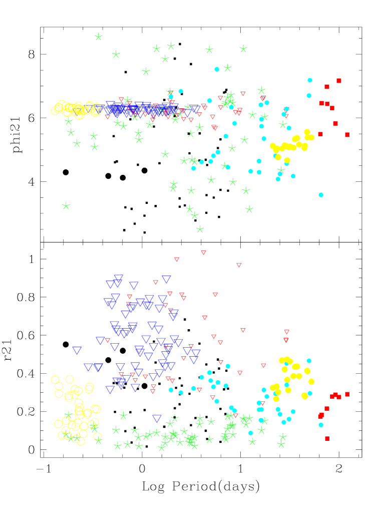
Figure 7: The classification obtained in the diagram $\log(\mbox{period})$, $\phi_{21}$ and $\log(\mbox{period})$, $R_{21}$. Symbols as in Fig. 8.

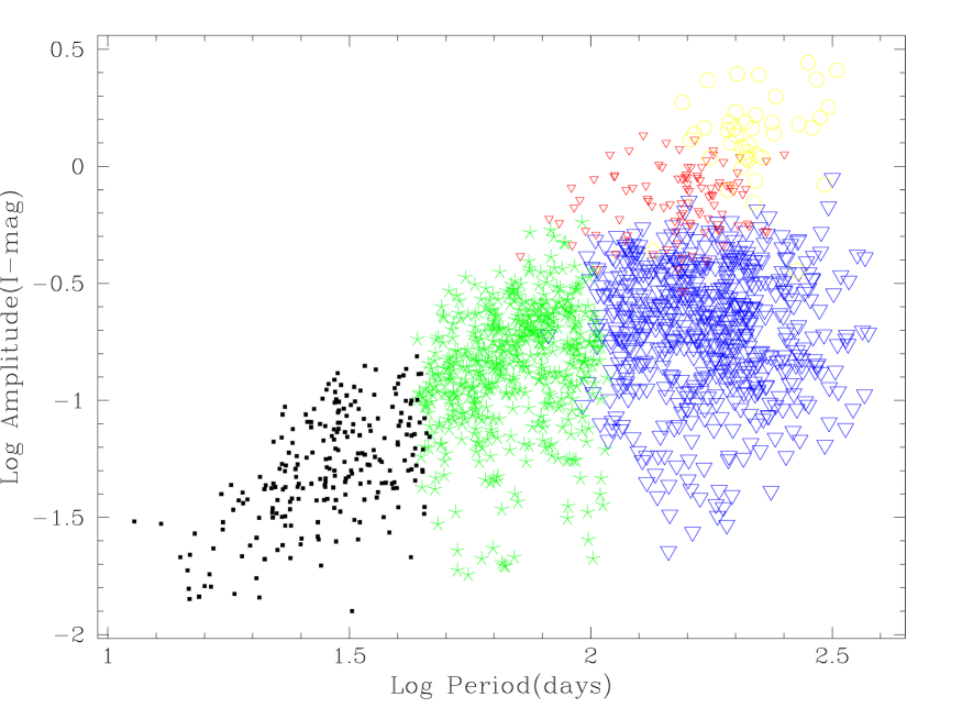
Figure 8: The classification obtained in the diagram $\log(\mbox{period})$, $\log(\mbox{amplitude})$ for the red giants. The moments of the distribution decomposition are used. The classifier forms 5 groups which can be identified to three general known variability types: small amplitude red variables (small black squares), Semi-regular variable stars (5 branch star, open triangles) and Mira stars (open circles).

For the subsample of 302 stars, the stars are classified in 9 groups. Certain groups appear to be very clean and others seem to contain more difficult cases. See Fig. 8 and Fig. 7 for the result of the classification in a $\log(\mbox{Period})-\log(\mbox{Amplitude})$ diagram and $\log(\mbox{Period})-\phi_{21}$ or $R_{21}$ diagram. We have:

• Eclipsing binaries ($\sim$192): One group with (63 stars) eclipsing binaries of EA and EB type. This group has no ambiguity of classification. Another group (36 stars) of EW type eclipsing binaries, includes very few potential pulsating stars (like $\delta$ Scuti stars) or Ap stars with very sinusoidal curves. The third group (38 stars) contains more difficult cases, a large majority are eclipsing binaries, some seem marginal, and others have clearly a wrong period.

• Cepheids ($\sim$19+13=32): We can find this type of variables in two different classes. One is very well defined (19 stars). Only one star seems to be peculiar in changing its amplitude. There are about 13 other cases which could be Cepheids, some undoubtedly recognizable to human eyes, while others are difficult to recognize.

• RR Lyrae stars ($\sim$ 4): probably one delta Scuti and 3 RR Lyrae of ab type, RR Lyrae of c types will be mixed with Eclipsing binaries of EW type.

• LPVs (Long Period Variable stars): 8 stars are classified in a group with poorly defined light curves, and with periods above 60 days. The time sampling is often sparse and does not cover many cycles of the light curve. The phase coverage often presents gaps.

• Small amplitude variables ($\sim$ 44): many light curves seem to be marginal cases. Very few unambiguous cases could be identified. However, it makes sense to have such a group. There are some $\alpha$CVn which could be present in this group. The mean amplitude of this group is of 0.04 I-mag.

• The last group ($\sim$ 58) is also composed of difficult cases but of larger amplitude (mean amplitude is 0.12 I-mag) than the previous one. Here the variability is strongly detected. It is worth noting that the formation of this group is a remarkable aspect of the classifier. Instead of spreading those objects among well defined classes, it is putting them in a separate group.

In total from this classification there are 5 groups out of 9 which contain clear cases with an error of classification below 7%, 2 groups, with some mixed classification, one group of small amplitude variables which can be caused by many different effects, and one group with very difficult cases.

The RR Lyrae stars, because of the limiting magnitude of the ASAS survey, are too faint to be numerously detected. Indeed the SDSS survey (Ivezic et al. 2000) shows that the halo RR Lyrae stars are very rare below I-mag 13. Therefore, only 3-4 RR Lyrae stars are found in the sample. The classification algorithm sometimes identifies the RRab type, depending on the precision that we estimated for the period, but these stars are not forming a stable class. However, it is remarkable that the program can form a new group with such a small number of stars (about 1% of the sample). The classification was found to be sensitive to error parameters and sometimes group RR Lyrae are lost.

Beltrame and Poretti (2002) found that ASAS star 112843-5925.7 (HD304373) is a double mode Cepheid, the second one detected in our Galaxy, pulsating in the first and second overtones or radial mode. In our study, unfortunately the period search was limited for that star to a frequency interval up to 0.5, missing the main peak of this short period pulsator (Period $=$ 1.08 [1/day]). It is classified in the group of stars which is a mix of pulsating and eclipsing.

The second group of 1429 stars, where we use the moments of the distribution, is divided by Autoclass in 5 groups. The classification divides those stars into: SARV ($\sim$230), SR ($\sim 1158=102+484+572$), Mira ($\sim$41).

With these groups it is difficult to determine error levels since the classification is extremely difficult to establish. There are some amusing case, the star ASAS180057-2333.8 is in the group of Mira stars, but is clearly a long period eclipsing binary.

The catalogue, the light curves, and folded curves on individual basis and on class basis can be seen at the first author’s website.

The eclipsing binaries have recomputed solutions where the initial period is doubled since the Lomb-Scargle algorithm usually gives half of the true period. The star 144245-0039.9 even has a factor 4 between the true period and the period found by the Lomb algorithm.

9 Conclusion

We have developed a scheme for general and automated classification for the periodic variable stars of ASAS 1-2 data set. Of course every survey has its own properties, so even if the approach is transferable in its principles, it probably requires modifications for every data set. The general method, however, can easily be applied to larger databases.

The work was broken into three parts: a) Selection of periodic objects, b) modeling that subsample with Fourier series or with simpler parameters like moments of the distribution and c) application of the ”Autoclass” Bayesian classifier. At every step it is critical to check the quality of the analysis, to interact with the data and to visualize data or the defined parameters.

Other studies are awaited (for example Woźniak et al. 2001), using different methods. It is important to compare the efficiency of the methods, their capability to detect new classes, their error levels, and their CPU consumption. It might be interesting to apply such a Bayesian classifier to the data of ASAS 3 and compare it with the results of Pojmański (2002, 2004).

At present, and in the very near future, there are several good opportunities to apply such a classification method to other data sets:

• ASAS continues to survey the sky.

• The HAT project (Bakos et al. 2002) has released data (Hartman et al. 2004)

• The Magellanic Clouds data of OGLE-II (Żebruń et al. 2002) is available (58’000 variable stars), as well the 49 bulge fields from OGLE-II (Woźniak et al. 2002). The classification of bulge field 1 has been done by Mizerski and Bejger (2002), specific extractions of eclipsing binaries, RR Lyrae, Cepheids stars have been accomplished for the Magellanic clouds.

• The third phase of OGLE, OGLE-III, is functional and is taking data. The data rate is multiplied by a factor of 10 with respect to OGLE-II.

Real time detection and classification of phenomena such as supernovae will require additional software development to be scientifically valuable. For example, OGLE has possessed an Early Warning System (EWS) since 1994 and received further development in 2003 to include the detection of the effect of planets in a microlensing event. It is envisioned that the OGLE data will be put into the public domain within 24 hours. If so, OGLE-III opens the possibility for anyone to make quasi-real time detection of variable phenomenon.

ASAS also has an Alert service. The photometric reduction pipeline is available in real time within 5 minutes. The current service is focused on the monitoring of cataclysmic variable stars.

Similar software has to be developed for large surveys from the ground and from space like the GAIA mission (ESA 2000), so it is important to gain knowledge of different classification methods.

10 Acknowledgements

We are thankful for the help, comments and encouragements of B. Paczyński, C. Alard, A. Gautschy, M. Grenon, Z. Ivezic and G. Pojmański. Our thanks go to M.C.S. Peterson for English corrections, W. O’Mullan and A. Dartois for their help in Java programming. The software SM (Lupton and Monger, 1997) was widely used for this research. Partial support for this project were provided by the Swiss National Science Foundation, the NSF grant AST-XXXXXX and the Carnegie Institution of Washington, Dept. of Terrestrial Magnetism.

Table 1: Results of the classification (exctract, the full catalogue is available in the online version of the article). The columns are the ASAS ID (equatorial coordinates in equinox 2000), mean $I$ magnitude $\bar{I}$, standard error $\sigma_{I}$, the number of measurements $N$, the period, the amplitude, the amplitude ratio R21, the phase difference $\phi_{21}$, the number of harmonics $nh$, the classe $cl$, the probability of membership Prob.

ASAS ID	$\bar{I}$	$\sigma$	$N$	Period	Ampl	$R21$	$\phi_{21}$	nh	cl	Prob
$005759+0034.7$	10.444	0.028	1204	0.7980	0.076	0.396	6.242	6	3	0.42
$015647-0021.2$	11.041	0.047	417	0.5427	0.108	0.102	7.996	2	1	0.43
$030201-0027.2$	10.311	0.049	1133	3.1062	0.118	0.052	5.505	2	1	0.47
$034803-0023.5$	10.793	0.032	1314	7.0156	0.045	0.187	6.816	2	2	0.47
$044830+0017.9$	12.205	0.124	1457	0.2250	0.294	0.307	6.374	3	4	0.49
$044944+0056.0$	11.447	0.086	862	0.7116	0.204	0.028	6.557	2	1	0.50
$045017+0100.7$	11.379	0.091	503	0.2056	0.224	0.288	6.294	2	4	0.50
$045024+0013.2$	9.913	0.015	1530	6.2548	0.015	0.040	3.738	2	2	0.51
$045128-0032.7$	7.596	0.013	1534	0.7818	0.022	0.037	3.143	2	2	0.51
$045206-7043.9$	10.542	0.086	312	1.1724	0.193	0.758	6.266	4	0	0.52
$045423-7054.1$	11.773	0.175	423	34.4540	0.566	0.385	5.068	5	6	0.53
$045506-6728.5$	12.630	0.194	267	29.8318	0.511	0.366	4.665	3	6	0.53
$045511-0101.7$	10.247	0.023	792	3.1366	0.031	0.128	7.689	2	2	0.54
$045702-6759.7$	12.065	0.123	517	45.1273	0.322	0.279	5.124	2	6	0.55
$045712-6723.2$	12.162	0.147	273	22.7070	0.387	0.293	4.809	4	5	0.55
$045720-8023.0$	11.615	0.228	3448	0.1835	0.721	0.368	6.321	6	4	0.56
$045728-7033.1$	12.053	0.113	676	0.8249	0.383	0.866	6.301	5	0	0.56
$045750-6957.4$	12.354	0.147	309	23.3178	0.583	0.331	5.039	5	6	0.57
$045810-6957.0$	11.839	0.197	637	39.3889	0.575	0.385	5.162	5	6	0.57
$045817-0013.9$	10.942	0.047	1296	0.2522	0.095	0.083	6.223	2	4	0.58
$045832-7020.8$	11.970	0.177	621	35.6997	0.607	0.435	5.332	5	6	0.59
$045836-7006.6$	12.591	0.183	295	17.2697	0.567	0.313	5.349	2	5	0.59
$045914-6935.7$	11.061	0.100	700	0.3289	0.266	0.109	5.087	3	1	0.59
$045941-6927.4$	12.541	0.238	596	31.8223	0.833	0.463	5.099	4	6	0.60
$050047-7029.8$	10.702	0.119	706	0.1937	0.340	0.169	6.318	3	4	0.60
$050327-6909.0$	12.473	0.172	264	21.2662	0.498	0.324	5.121	4	6	0.61
$050527-6743.2$	9.906	0.083	694	2.0243	0.240	0.364	6.509	4	3	0.62
$050556-6810.7$	11.114	0.070	391	7.3966	0.138	0.109	6.643	2	1	0.62
$050558-6810.5$	11.220	0.075	274	7.3957	0.128	0.174	7.570	2	1	0.64
$050648-7002.2$	11.913	0.204	644	47.4545	0.643	0.414	5.557	4	6	0.66
$050720-7027.2$	12.642	0.293	528	26.3391	0.988	0.468	5.035	6	6	0.66
$050818-6846.8$	11.497	0.106	578	30.5056	0.251	0.312	5.087	2	6	0.67
$050920-7027.4$	11.914	0.205	675	37.5444	0.636	0.436	5.369	5	6	0.67
$051608-6815.5$	9.708	0.023	699	2.1377	0.028	0.169	6.057	2	2	0.67
$051833-6813.6$	10.089	0.176	698	0.1427	0.550	0.294	6.326	4	4	0.67
$052507-6738.6$	11.326	0.186	1152	48.0851	0.536	0.411	5.386	5	6	0.67
$052557-7011.1$	10.556	0.059	1388	1.5803	0.132	0.010	6.235	2	1	0.68
$052650-8135.2$	7.953	0.142	2491	0.2308	0.406	0.221	6.229	3	4	0.68
$052655-6958.9$	12.102	0.120	508	28.1222	0.316	0.421	5.134	2	6	0.69
$052832-6836.2$	10.525	0.042	700	0.2884	0.078	0.317	6.362	2	4	0.71
$053014-6926.2$	12.456	0.153	417	23.0127	0.405	0.266	4.989	4	6	0.71
$053120-7057.5$	11.554	0.148	497	52.5205	0.438	0.356	5.384	3	6	0.71
$053502-6843.7$	11.875	0.095	669	0.5432	0.216	0.636	6.314	3	0	0.72
$053936-7958.6$	10.418	0.040	3946	0.9208	0.114	0.410	6.262	6	0	0.72
$053959-6828.7$	10.765	0.165	693	0.1811	0.481	0.272	6.309	3	4	0.73
$055122-6812.8$	11.747	0.120	682	0.3218	0.307	0.124	5.431	2	1	0.73
$055602-0003.8$	10.814	0.036	1374	9.8757	0.059	0.405	6.266	2	3	0.73
$055624+0013.0$	9.471	0.014	1376	1.3206	0.013	0.567	5.726	2	2	0.74
$055701+0025.7$	9.718	0.036	1375	0.1411	0.098	0.134	6.274	3	4	0.75
$055850-0026.5$	10.004	0.022	1375	0.5301	0.026	0.198	4.603	2	2	0.75

Figure 1: The histogram of the number of measurements per star.

Figure 2: The normalized histogram of time intervals between successive measurements. We can see the regular nightly observing pattern. However, there are other characteristic time intervals for instance $\sim$5 minutes or $\sim$45 minutes.

Figure 3: Histogram of the difference between the last and first epoch. The star sample is somewhat heterogeneous, but with many stars being covered over a period of nearly 3 years. However, those stars may have large intervals without observations.

Figure 4: Comparison of the periods, obtained by the Lomb algorithm on the data and when a parabolic fit is subtracted from the data, allows some aliases as well as unstable solutions to be identified.

Figure 5: The raw diagram $\log(\mbox{period})$, $\log(\mbox{amplitude})$. The diagram is dominated by red stars which seem to fall on a relation (or several neighbouring sequences).

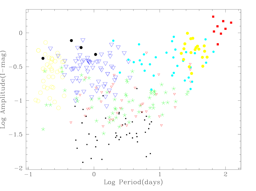
Figure 6: The classification obtained in the diagram $\log(\mbox{period})$, $\log(\mbox{amplitude})$. Red Giant stars are excluded from the classification. The Fourier decomposition is used. The colours description is for the online version. The symbols are: Eclipsing binaries: large blue open triangle, open yellow circles, red small open triangle; RR Lyrae: black large full circles; Cepheids: yellow small full circles, blue small circles; LPV: red full large squares; Small amplitude variables: small black squares. Uncertain cases: green 5 branch star.

Figure 9: Three examples (on one line) of each of the 12 major classes are represented. We have: 1) eclipsing binaries ($\sim$ EA, EB types), 2) eclipsing binaries ($\sim$EW types), 3) eclipsing binaries (more marginal cases), 4) cepheids, 5) cepheids (with more marginal cases), 6) LPVs, 7) RR Lyrae candidates, 8) various case class, 9) small amplitude variables, 10) SARVs, 11) SRs, 12) Miras. On the right of the folded curve is the ASAS coordinate (equinox 2000), on the left is the period in days.

References

- [1] Bakos G. Á., Lázár J., Papp I., Sári P., Green E. M., 2002, PASP, 114, 974
- [2] Belokurov V., Evans N. W., Du Y. L., 2003, MNRAS, 341, 1373
- [3] Beltrame M., Poretti E., 2002, A&A, 386, L9
- [4] Cheeseman P., Stutz J., 1996, in Fayyad U. M., Piatetsky-Shapiro G., Smyth P., Uthurusamy R., eds, Advances in Knowledge Discovery and Data Mining, Bayesian classification (AutoClass): Theory and results. AAAI Press/MIT Press, p. 61
- [5] ESA, 1997, The Hipparcos and Tycho Catalogues, ESA SP-1200
- [6] ESA, 2000, GAIA (Concept and Technology Study Report), ESA-SCI(2000)4
- [7] Eyer L., Grenon M., 1997, ESA SP-402, 467
- [8] Eyer L., 1998, PhD Thesis, Geneva University
- [9] Eyer L., Bartholdi P., 1999, A&ASS, 135, 1
- [10] Eyer L., Genton M., 1999, A&ASS, 136, 421
- [11] Eyer L., Blake C., 2002, in Aerts C., Bedding T., Christensen-Dalsgaard J., eds, ASP Conf. Ser. 259, Radial and Nonradial Pulsations as Probes of Stellar physics. Astron. Soc. Pac., San Francisco, p. 160
- [12] Goebel J., Stutz J., Volk K., Walker H., Gerbault F., Self M., Taylor W., Cheeseman P., 1989, A&A, 222, L5
- [13] Hartman J. D., Bakos G., Stanek K., Noyes R. W., 2004, preprint (astro-ph/0405597)
- [14] Ivezic Z. et al., 2000, ApJ, 120, 963
- [15] Kholopov P.N., 1985, General Catalogue of Variable Stars
- [16] Koen C., Eyer L., 2002, MNRAS, 331, 45
- [17] Lomb N.R., 1976, Ap&SS, 39, 447
- [18] Lupton R.H., 1993, Statistics in theory and practice. Princeton Univ. Press
- [19] Lupton R.H., Monger P., 1997, The SM Reference Manual, (URL: http://www.astro.princeton.edu/rhl/sm/sm.html)
- [20] Minniti D. et al., 1998, in Takeuti M., Sasselov D. D., eds, Pulsating Stars. Universal Academy Press, Tokyo, p. 5
- [21] Mizerski, T., Bejger, M., 2002, AcA, 52, 61
- [22] Paczyński, B., 1997, in Ferlet R., Maillard J.-P., Raban B., eds, Variables Stars and the Astrophysical Returns of the Microlensing Surveys. Editions Frontières, France, p. 35
- [23] Paczyński B., 2000, PASP 112, 1281
- [24] Paczyński B., 2001, in Banday A. J., Zaroubi S., Bartelmann M., eds, Mining the Sky. Springer, Berlin, p. 481
- [25] Percy J. R., Wilson J. B., Henry G. W., 2001, PASP, 113, 983
- [26] Piquard S., Halbwachs J.-L., Fabricius C., Geckeler R., Soubiran C., Wicenec A., 2001, A&A, 373, 576
- [27] Pojmański G., 2000, AcA, 50, 177
- [28] Pojmański G., 2002, AcA, 52, 397
- [29] Pojmański G., 2003, AcA, 53, 341
- [30] Pojmański G., Maciejewksi G., 2004, preprint (astro-ph/0406256)
- [31] Press W. H., Teukolsky S. A., Vetterling W. T., Flannery B. P., 1992, Numerical Recipes in Fortran. Cambridge University Press
- [32] Rodriguez E., López-González M. J., López de Coca P., 2000, A&ASS, 144, 469
- [33] Schwarzenberg-Czerny A., 1991, MNRAS, 253, 198
- [34] van Loon J.Th., 2002, in Aerts C., Bedding T., Christensen-Dalsgaard J., eds, ASP Conf. Ser. 259, Radial and Nonradial Pulsations as Probes of Stellar physics. Astron. Soc. Pac., San Francisco, p. 458
- [35] Woźniak P. et al., 2001, AAS, 199
- [36] Woźniak P., Udalski A., Szymański M., Kubiak M., Pietrzyński G., Soszyński I., Żebruń K., 2002, AcA, 52, 129
- [37] Woźniak P. et al., 2004, preprint (astro-ph/0401217)
- [38] Wray J.J., Eyer L., Paczyński B., 2004, MNRAS, 349, 1059
- [39] Żebruń K., et al., 2001, AcA, 51, 317