Dust Reddening in Sloan Digital Sky Survey Quasars

Abstract

We explore the form of extragalactic reddening toward quasars using a sample of 9566 quasars with redshifts $0<z<2.2$, and accurate optical colors from the Sloan Digital Sky Survey (SDSS). We confirm that dust reddening is the primary explanation for the red “tail” of the color distribution of SDSS quasars. Our fitting to 5-band photometry normalized by the modal quasar color as a function of redshift shows that this “tail” is well described by SMC-like reddening but not by LMC-like, Galactic, or Gaskell et al. (2004) reddening. Extension to longer wavelengths using a subset of 1886 SDSS-2MASS matches confirms these results at high significance. We carry out Monte-Carlo simulations that match the observed distribution of quasar spectral energy distributions using a Lorentzian dust reddening distribution; 2% of quasars selected by the main SDSS targeting algorithm (i.e., which are not extincted out of the sample) have $E_{B-V}>0.1$; less than 1% have $E_{B-V}>0.2$, where the extinction is relative to quasars with modal colors. Reddening is uncorrelated with the presence of intervening narrow-line absorption systems, but reddened quasars are much more likely to show narrow absorption at the redshift of the quasar than are unreddened quasars. Thus the reddening towards quasars is dominated by SMC-like dust at the quasar redshift.

1 Introduction

The discovery of a very red population of radio-selected quasars, and studies of the color distribution of quasars (Webster et al., 1995; Brotherton et al., 2001; Francis et al., 2001; Richards et al., 2001; Gregg et al., 2002; White et al., 2003) suggest that a significant population of red quasars exists. This red population could arise from several sources: an intrinsically red continuum, an excess of synchrotron emission in the red, intervening absorption by galaxies along the line of sight, and dust extinction in the host galaxy or central engine of the quasar itself. With its small photometric errors and very large quasar sample selected in the $i$-band, the Sloan Digital Sky Survey (SDSS; York et al. 2000) is well-suited to explore the properties of mildly dust-reddened quasars. Richards et al. (2003) used redshift-independent criteria to quantify the “redness” of SDSS quasars based on their optical colors, and concluded that the core of the color distribution was consistent with a range of intrinsic slopes of quasar continua, while the extended red tail was the sign of dust located predominantly at the redshift of the quasar. We extend this work in the present paper, looking both for the change in slope and the induced curvature expected in the quasar spectral energy distribution in the presence of dust reddening. Our aim is to characterize the nature of the dust giving rise to the observed reddening, and to constrain its intrinsic distribution. For example, Gaskell et al. (2004) have recently proposed that quasars have a nuclear reddening curve which is flat in the ultraviolet, in contrast to the well-studied curves of the Milky Way (MW), the Large Magellanic Cloud (LMC), and the Small Magellanic Cloud (SMC).

The SDSS and the sample of quasars we use are described in § 2. We fit the colors to derive the slope and curvature in § 3, and compare our results with simple models for the distribution of dust extinction. Our conclusions are presented in § 4.

2 The Sloan Digital Sky Survey and Sample Selection

The quasars analyzed here were selected from the SDSS imaging survey, which uses a wide-field multi-CCD camera (Gunn et al., 1998) which produces accurate photometry in five broad bands ($ugriz$) which cover the optical window from 3000 to 10,000Å. Quasar candidates are selected (Richards et al., 2002) based on their $ugriz$ colors (Fukugita et al., 1996; Lupton, Gunn, $\&$ Szalay, 1999; Hogg et al., 2001; Smith et al., 2002; Stoughton et al., 2002) and as optical matches to quasars from the VLA “FIRST” survey (Becker et al., 1995), and are spectroscopically observed in the wavelength range $3800<\lambda<9200$ Å. The quasar selection is not limited to UV-excess objects; all objects lying sufficiently far from the stellar locus in color-color space brighter than the $i$ band magnitude limit are selected, with the exception of objects in certain exclusion boxes; see Richards et al. (2001).

Point-spread-function magnitudes were extracted as explained by Lupton et al. (2001), and magnitudes have been corrected for Galactic extinction using the maps of Schlegel, Finkbeiner, $\&$ Davis (1998). See Stoughton et al. (2002) for details of the spectroscopic system and analysis pipelines. Astrometric calibration is detailed in Pier et al. (2003) and the spectroscopic plate tiling procedure in Blanton et al. (2003).

The sample consists of objects from the SDSS first data release (DR1; Abazajian et al. 2003) cataloged as quasars by Schneider et al. (2003). Objects with $z>2.2$ are not included, in order to avoid contamination of the analysis of spectral shapes and potential reddening by the effects of Ly$\alpha$ forest absorption. We have included objects showing broad absorption lines in their spectra, although we leave to future work to explore whether their dust properties differ from those of “normal” quasars.

At low redshift ($z\lesssim 0.3$), most SDSS AGNs have low luminosity and do not strongly outshine their host galaxies. Indeed, many of the reddest objects are dominated by the spectrum of the host galaxy, showing strong stellar absorption lines. To eliminate the potentially contaminating objects, we retained only objects targeted as low-$z$ quasars selected by the final version of the quasar target selection algorithm (with $M_{i}<-22$ in a cosmology in which $H_{0}=70$ km s^-1 Mpc^-1, $\Omega_{M}=0.3$, $\Omega_{\Lambda}=0.7$, and in which quasar SEDs have $f_{\nu}\propto\nu^{-0.5}$). Visual inspection confirmed that the eliminated objects were primarily objects in which the host galaxy dominated the spectrum, and that there are only a few objects in the retained sample which show stellar absorption systems in their spectra. The final sample consists of 9566 quasars.

This sample was matched to the Two Micron All Sky Survey (2MASS; Skrutskie et al. 1997) all-sky point source catalog using a matching radius of 3^′′ (Schneider et al., 2003). The addition of 2MASS observations extends the wavelength baseline by adding $J$, $H$, and $K$ band photometry. Typical magnitude errors in each band are $\sim 0.1-0.15$ mag. This sample again includes only objects with $0\leq z\leq 2.2$, and the final sample includes 1886 quasars.

Richards et al. (2003) show that for $E_{B-V}=0.1$, the completeness of the SDSS quasar target selection is at least 90$\%$ at $z<2$ for objects luminous enough that extinction does not cause them to fall below the magnitude limit. In this paper, we will be sensitive to objects with moderate amounts of dust reddening, as objects with extreme dust reddenings ($E_{B-V}\gtrsim 0.5$) will be difficult to recognize as quasars and will usually be extincted out of the sample. The fraction of quasars which are so heavily reddened has been estimated as 16% based on SDSS data (Richards et al., 2003) and 15%-22.5% based on a 2MASS+VLA-FIRST survey (Glikman et al., 2004).

3 Fitting Reddening Models to Quasar Colors

3.1 Colors as a Function of Redshift

We follow the convention of Richards et al. (2001; 2003), and define “red” quasars using colors relative to those of typical quasars as a function of redshift. These papers used median colors as a function of redshift; however, a population of dust-reddened quasars will shift the median quasar colors redder, but will leave the mode unaffected. Thus we use the modal colors as a function of redshift in this paper. The DR1 quasars were sorted by redshift and then split into bins of width 0.05 in redshift $z$. Each quasar’s color was taken to be a Gaussian centered at the given value for that quasar, with a standard deviation equal to the photometric error for that particular quasar and color. All Gaussians in the bin were then summed and the peak of the resulting distribution was used as the modal color of the bin. Bin sizes as large as 0.1 gave similar results, whereas bins with a significantly smaller numbers of quasars per bin gave noise-dominated results.

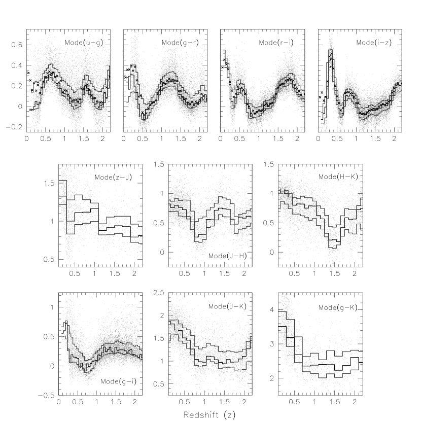
Figure 1: The dependence of modal colors on redshift. Points plot individual quasar colors, and the lines in each box show the modal color and the outer quartiles as a function of redshift. The top four boxes are the SDSS colors and the center three boxes are colors obtained from the SDSS-2MASS matched sample. The bottom three boxes show the commonly used reddening indicators $g-i$, $J-K$, and $g-K$ as determined directly. The modes $u-g$, $g-r$, $r-i$, $i-z$, and $g-i$ were taken in bins of $\Delta z=\pm 0.05$. Modes $J-H$, $H-K$, and $J-K$ use bins of $\Delta z=\pm 0.1$, and $z-J$ and $g-K$ use bins of $\Delta z=\pm 0.2$. For comparison, the median color-redshift relation of Richards et al. (2003) is shown for the SDSS colors as $\times$’s.

The modes of the 2MASS colors $J-H$, $H-K$, and $J-K$ were found using a sample of 5162 quasars from Table 1 of Veron-Cetty & Veron (2001) which have 2MASS-point source catalog counterparts within 4″. A false coincidence rate of only 1.6% is expected with this matching radius (Barkhouse & Hall, 2001). Due to the smaller number of quasars, the bin size was taken to be 0.1 in redshift. The modes in $z-J$ and $g-K$ were taken from the SDSS-2MASS matched sample, and a bin of 0.2 was used due to the still smaller sample size. Table 1 and Figure 1 show the modal colors as a function of redshift for the four SDSS colors ($u-g$, $g-r$, $r-i$, $i-z$), three SDSS-2MASS matched colors ($z-J$, $J-H$, $H-K$), and three colors commonly used as reddening indicators ($g-i$, $J-K$, and $g-K$, a color very close to $B-K$). We show for comparison the median colors of Richards et al. (2001), which tend to be biased to the red (by $\sim 0.025$ mag), as expected for a distribution with a red tail.

3.2 Fit Construction

We define relative colors of each quasar by subtracting the modal color at that redshift from the quasar’s observed colors; this corrects the colors for the effects of emission lines redshifting through the SDSS and 2MASS filters; in essence, this applies a $k$-correction for the emission lines.

Adding these relative colors to a fixed $i$ magnitude ($i=0$) gives relative $ugrizJHK$ magnitudes: a quasar at the mode of the color-redshift relation will thus have all relative magnitudes equal to zero. Deviations of the modal magnitudes from zero can be modeled as due to reddening; as reddening is greater at shorter wavelengths, we expect a curvature in the spectral energy distributions. To quantify this, we fit a second-order Chebyshev polynomial to the relative magnitudes of each quasar in turn as a function of the logarithm of wavelength. The effective wavelengths of the filters are 3541, 4653, 6147, 7461, 8904 Å, respectively, in $ugriz$, and 12350, 16620, and 21590 Å, respectively, in $JHK$ (the variation in effective wavelength with the shape of the SED is negligible for our purposes). We fit the photometry rather than the SDSS spectra to measure the reddening because the photometry has higher signal-to-noise ratio, better calibration (cf., Abazajian et al. 2004), and a longer wavelength baseline.

The Chebyshev fit to each quasar is carried out with $\chi^{2}$ minimization, using the PSF magnitude errors in each band (with a floor of 0.01 mag). The Chebyshev polynomials are designed to give statistical independence to the derived slope and curvature for each quasar. We use the notation $c_{2}$, $c_{1}$, $c_{0}$, for the best-fit coefficients of the Chebyshev polynomials of second, first, and zeroth order, respectively. Simple changes in the power-law slope will affect $c_{1}$, while $c_{2}$ will remain close to zero. Dust reddening causes curvature in the spectrum, and should give positive values of $c_{2}$ correlated with $c_{1}$. A “normal” quasar with colors close to the mode will have relative magnitudes all close to zero, and thus $c_{1}=c_{2}=0$. In what follows, we will show results from our full sample of 9566 quasars, where the fit is restricted just to the SDSS filters, and to the subset with 2MASS photometry, where the fit includes $JHK$ as well.

The data do indeed call for a curvature ($c_{2}$) term. Figure 2 shows the improvement in $\chi^{2}$ in second-order fits to the SDSS photometry alone, relative to a linear fit. The addition of a single fitting parameter typically improves $\chi^{2}$ by of order unity if the data are well-fit without this parameter. For objects with large $c_{2}$, the improvement in $\chi^{2}$ is typically much greater than unity.

3.3 Fit Results and Comparison to Dust Reddening Models

Figure 3 shows the relationship between curvature $c_{2}$ and slope $c_{1}$ for the objects in our full sample, fitting to the SDSS photometry alone. Again, the modal quasar has $c_{1}=c_{2}=0$ at all redshifts. The distribution of the quasars is shown as contours and outlying points, with a symmetric distribution about a curvature and slope of 0, and a tail. Note the strong correlation between $c_{1}$ and $c_{2}$ in the tail, as expected with dust reddening.

We compare the observed correlation of $c_{1}$ and $c_{2}$ with those derived from SMC-like, LMC-like, MW-like (Galactic), and Gaskell et al. (2004) dust reddening laws. We use the numerical formulations of Pei (1992) for the Galactic and Magellanic laws. (There is, of course, considerable spatial variation in the dust extinction curve of the Milky Way and of the LMC (Draine, 2003); the curves we refer to in this paper can be thought of as the “traditional” MW, LMC 30 Doradus region, and SMC “bar” extinction curves.) For each reddening law, we simulate reddened quasar colors by beginning with a ‘quasar’ with all four SDSS modal colors set to 0. We then determine the changes to the colors that would result from applying each of the four reddening laws with $0\leq E_{B-V}\leq 0.8$ (in bins of 0.05) to the modal quasar at $0\leq z\leq 2.2$ (in bins of 0.2). In all there are 204 such simulated colors for each reddening law (17 $E_{B-V}$ bins times 12 redshift bins). The reddening we apply here is relative to the modal quasar, and therefore is in addition to any reddening experienced by the modal quasar itself. We explicitly modeled extinction only at the quasar redshifts (cf., § 3.5 below), However, the relative colors we use are independent of redshift, so a quasar with associated dust at $z=1$ and a quasar at $z=2$ with the same amount of intervening dust at $z=1$ both have the same shift in the $c_{1}$ vs. $c_{2}$ diagram. That is, our simulated $c_{1}$ and $c_{2}$ values describe the effects of both associated and intervening dust.

These simulated relative colors were then fit to the Chebyshev polynomials to obtain values of the slope and curvature ($c_{1}$ and $c_{2}$). The results are shown in Figure 3. Model quasars reddened by an SMC-like law appear as solid dots, those reddened by an LMC-like law as crosses, those reddened by a MW law as triangles, and those reddened by the Gaskell et al. (2004) law as plus signs. The SMC law is nearly a power law in wavelength, and in particular does not have a 2175Å feature, which is why all the model points lie along a single locus independent of redshift.

The observed distribution is extended along the axis predicted by an SMC-like dust reddening law. Although objects reddened by LMC-like, MW-like, or Gaskell et al. (2004) laws can appear in the tail, the majority of objects with these reddening laws fall far from the observed tail. For additional emphasis, the simple least-squares linear fit to the simulated quasars reddened by the SMC-like law is shown in the $c_{1}$, $c_{2}$ space. Although our data do not exclude the possibility that there is some component of dust reddening in at least some of our objects which follows other reddening laws, it appears that SMC-like extinction curves dominate the reddening along most quasar sightlines. Figure 4 makes explicit the relationship between reddening, $E(B-V)$, and $c_{1}$ and $c_{2}$ for the SMC law; points of a given $E(B-V)$ at different redshifts are connected. The equivalent plot for the MW extinction law is not at all linear, because of the influence of the 2175Å feature.

This analysis has focused purely on the reddening of quasars; we have not modeled here the extinction of quasars which would take them below our magnitude limit, causing them to drop out of the sample. However, extinction does not affect our conclusion about the dominance of SMC-like reddening along quasar sightlines. At $z<2.2$, the $i$-band selection of the SDSS corresponds to selection at rest-frame $\lambda>2330$ Å. The SMC, LMC and MW extinction curves for a fixed reddening $E_{B-V}$ agree within 10% at such wavelengths. Since the SDSS can detect intrinsically very luminous quasars with SMC-like reddenings of up to $E_{B-V}\simeq 0.5$ (Hall et al., 2002), it can also detect quasars with similar reddenings but LMC-like or MW-like extinction curves. Thus the absence of highly reddened quasars with the slope and curvature parameters expected for LMC-like or MW-like extinction curves must be due to the scarcity of dust with such extinction curves along the sightlines to quasars.

The column density of gas $N_{H}$ required to generate a given dust reddening $E_{B-V}$ is a function of the extinction curve. Because the SMC-LMC-MW extinction law sequence is probably at least in part a metallicity sequence, MW-like dust has $E_{B-V}/N_{H}$ approximately nine times larger than SMC-like dust; and LMC-like dust has $E_{B-V}/N_{H}$ approximately 2.25 times larger than SMC-like dust (Diplas $\&$ Savage, 1994; Koorneef, 1982; Bouchet et al., 1985). Thus, the limiting $E_{B-V}\simeq 0.5$ to which the SDSS is sensitive will be reached at a lower column density for gas with MW- or LMC-like extinction curves than for SMC-like extinction curves. Since lower column density systems are likely to be more common than higher column density ones, the slope-curvature plane would show an excess of MW- and LMC-reddened objects even if all three reddening curves were equally common. The relative lack of such objects in spite of this effect means that SMC-like extinction is truly dominant along quasar sightlines.

The Chebyshev fitting procedure was next applied to SDSS-2MASS matched quasars. Using the SDSS photometry for $ugriz$ magnitudes, and the 2MASS photometry for $JHK$ magnitudes, each of the 1886 quasars in this sample had seven colors instead of the four for SDSS-only quasars (adding $z-J$, $J-H$, and $H-K$). The baselines are extended by a factor of $\sim 3$ at the cost of larger photometric uncertainties, but this increases the signal-to-noise ratio of the Chebyshev coefficients by a factor of $\sim 3$. SDSS colors were normalized using the modes derived from the DR1 quasar sample, the $J-H$ and $H-K$ 2MASS colors were normalized using the modes derived from the Veron-Cetty & Veron (2001) 2MASS quasar sample, and $z-J$ colors were normalized using modes derived only from the 1886 quasar SDSS-2MASS matched sample (Figure 1). The Chebyshev polynomials were recalculated for the new baselines and then used as above to fit to the relative colors. The results are plotted in Figure 5. Again, “modal” quasars with $0\leq z\leq 2.2$ and $0\leq E_{B-V}\leq 0.8$ were simulated using SMC-like, LMC-like, MW-like, and Gaskell et al. (2004) dust reddening laws, and the results are overlaid. The extension of the contours of the observed distribution along the axis predicted by SMC-like reddening is again strong, although the distinction between the reddening laws is not as marked over this longer wavelength range (the strong curvature induced by the 2175 Å “bump” is “averaged out” over the longer wavelength baseline).

3.4 Monte Carlo Simulation of the Reddening Distribution

The $E_{B-V}$ values derived from direct fits to the photometry of individual objects are degenerate with other parameters, such as varying emission line strengths and the continuum power-law slope of the quasar spectrum. Thus we cannot infer the distribution of $E_{B-V}$ directly from these fits. Instead, we simulate the quasar population with various models for reddening and compare with the observed population. In this analysis, we are just modeling the effects of reddening; we do not attempt to include the effects of extinction, which would cause objects to drop out of the sample.

For each quasar in the sample, we take its redshift as given, and start by setting its colors to the mode at that redshift. We model three contributions to the relative colors: deviations in the continuum power-law slope of the intrinsic spectrum, SMC-like dust reddening at the quasar redshift, and photometric deviations from the “modal” quasar. For each quasar, we generate a random intrinsic slope deviation, $E_{B-V}$ value, and photometric deviations, each according to an assumed probability distribution. We assume that these probability distributions are independent of redshift and one another.

The photometric deviations model includes uncertainties in the determination of the modal colors and intrinsic deviations about those modal colors (e.g. from variations in emission line strength), as well as the PSF magnitude errors for each object. We assume the photometric deviations to be normally distributed around zero, with standard deviation ($\sigma_{error}$), to be determined. We follow Richards et al. (2003) and assume that the deviations from the modal power law slope $\alpha$ are also normally distributed around zero, with standard deviation $\sigma_{\alpha}$ as a quantity to be determined.

The distribution of $E_{B-V}$ values is also peaked at zero, since the “modal” quasar always has relative colors equal to zero, and as such shows no curvature as is induced by dust reddening. The existence of the “red tail” in the quasar color distribution suggests that the distribution must be asymmetric about zero. Given the distribution of fitted $E_{B-V}$ values, degeneracies between $E_{B-V}$ and power-law slope at small values of $E_{B-V}$, and the existence of some significantly bluer-than-average quasars, we allow negative $E_{B-V}$ values, which correspond to quasars which have undergone less dust reddening than the modal quasar at their redshift. We assume that the negative half of the $E_{B-V}$ distribution is also Gaussian with standard deviation $\sigma_{\rm Gaussian}$, giving a rapid falloff at large negative values as we expect. The high-curvature tail is to be explained by dust reddening, so the falloff with positive $E_{B-V}$ must be less rapid than Gaussian. We test two forms for $P(E_{B-V}>0)$:

$$P(E_{B-V}>0)\propto\exp(-x)$$ (1)

$$P(E_{B-V}>0)\propto\frac{1}{1+x^{n}}$$ (2)

where $x\equiv\frac{E_{B-V}}{\sigma_{dust}}$ and $n$ and $\sigma_{dust}$ are treated as quantities to be determined. As this model is purely empirical, there is no reason that the characteristic width of the Gaussian ($E_{B-V}<0$) half of the distribution should be the same as that of the $E_{B-V}>0$ half, so we also fit for their ratio, $\frac{\sigma_{\rm Gaussian}}{\sigma_{dust}}$. Fitting to the histogram of $\Delta(u-g)$ gives an approximate Lorentzian ($n=2$) profile, with $\sigma_{dust}\sim 0.02$, so we take these values as initial guesses.

Once the entire model sample has been fitted, a two-dimensional Kolmogorov-Smirnov (K-S) test (Fasano $\&$ Franceschini, 1987; Peacock, 1983) was used to compare the results to the original distribution. The $D$-value is the largest fractional difference in the population of any one quadrant, after dividing the slope-curvature space into four quadrants at each point in turn and comparing the results; it quantifies the goodness of fit.

An iterative process was used to obtain final values for $n$, $\sigma_{dust}$, $\sigma_{error}$, $\frac{\sigma_{\rm Gaussian}}{\sigma_{dust}}$, and $\sigma_{\alpha}$. Several values of each parameter were given, each with fractional deviation $\sim 0.5$ from the initial values mentioned above, and the full simulation was repeated for all possible combinations of these values. The combination of values which gave the lowest $D$-value was taken as the seed for the next iteration. The same number of possible values for each parameter was tested with each subsequent iteration, but the range of the parameters (fractional deviation from the best value of the previous run) was decreased by a factor of 2 and was re-centered on the minimum $D$-value parameter combination of the previous iteration. The iteration continued until the fractional change in the minimum $D$-value of subsequent iterations was less than $10^{-3}$. The entire process was repeated with identical and different initial values to check the stability of the convergence.

The results of these simulations are shown in Figures 6 and 7. The figures show the contours of the observed distribution and those of the simulated distribution using the final values of $n$, $\sigma_{dust}$, $\frac{\sigma_{\rm Gaussian}}{\sigma_{dust}}$, $\sigma_{error}$ and $\sigma_{\alpha}$. The best-fit simulation average value of the K-S statistic $D$ is shown in Table 2, along with the best-fit values of the simulation parameters for each sample. We find for the SDSS sample a marginally better fit using the exponential profile, with $\sigma_{\alpha}\approx 0.11,\,\sigma_{error}\approx 0.065,\,\sigma_{dust}\approx 0.032\,{\rm and}\,\frac{\sigma_{\rm Gaussian}}{\sigma_{dust}}\approx 0.54$. The errors given in Table 2 represent the range of tested values which give $D$-values within $\pm 0.01$ with all other parameters held constant; these errors should be considered as heuristic only. We find similar values for the matched SDSS-2MASS sample, except for the much larger $\sigma_{error}\approx 0.18$ due to the larger 2MASS photometric errors. In both cases, the best-fit pseudo-Lorentzian profile is similar to the best-fit exponential profile.

The values of $\sigma_{\alpha}$ and $\sigma_{error}$ are reasonable. Richards et al. (2003) find $\sigma_{\alpha}=0.125$, between the values obtained for the SDSS and SDSS-2MASS samples and within the error bounds obtained. The quantity $\sigma_{error}$ is only a factor of two above the typical errors in the PSF magnitudes, due to the effects of photometric calibration uncertainty, possible errors in the determination of the modal colors with redshift, and intrinsic deviations about the mode from sources other than variations in slope and dust reddening.

The best-fit model is $\sigma_{dust}=0.03$ with $\frac{\sigma_{\rm Gaussian}}{\sigma_{dust}}=0.55$; the parameters are essentially identical for the two parameterizations of Equations 1 and 2. In this model, we expect less than 1% of all quasars in the sample to have $E_{B-V}>0.2$, 2% to have $E_{B-V}>0.1$, and $9_{-2}^{+4}$% to have $E_{B-V}>0.055$. Richards et al. (2003) estimated that $\sim 6$% of quasars at the observed SDSS flux limit have $E_{B-V}>0.055$, but given the large errors, this value is consistent with the above estimates. The structure of the profile is such that the fraction of quasars with $E_{B-V}>0.055$ is highly sensitive to the exact value of $\sigma_{dust}$. As Figures 6 and 7 show, this model does an excellent job of fitting the tails of the marginal distributions in $c_{1}$ and $c_{2}$. A quasar at $z=1$ with $E_{B-V}$ of 0.2 has an extinction in the $i$ band of 0.95 magnitudes for SMC-like reddening. Thus, the SDSS probes one magnitude fainter for unreddened quasars than for quasars reddened by $E_{B-V}=0.2$. Quasars with reddening as large as $E_{B-V}=0.5$ are very rare in our data, mostly because the surface density of quasars luminous enough to be reddened so heavily and still lie above the SDSS magnitude limit is very small.

3.5 Where is the Absorbing Material?

The characteristic extinction we find along quasar sightlines, $\sigma_{dust}=0.03$, corresponds to a characteristic column density of $N_{H}=1.31\pm 0.33\times 10^{21}$ cm^-2 for SMC-like extinction (Bouchet et al., 1985), a level detectable in X-ray observations only for very nearby quasars or very long exposures. This value is at least an order of magnitude larger than expected from intervening absorption alone, as follows. If we make the extreme assumption that the column density distribution of intervening absorbers follows a power law of index $-1.2$ (Rao $\&$ Turnshek, 2000) up to the SDSS reddened-quasar detection limit of $2.2\times 10^{22}$ cm^-2 (corresponding to $E_{B-V}=0.5$ for SMC extinction), then we find an average total intervening column density of $N_{H}=4.7\times 10^{19}$ cm^-2. Therefore, reddening along quasar sightlines is dominated by reddening at each quasar’s redshift, whether in the region of the central engine or elsewhere in the quasar host galaxy. There are certainly examples of individual quasars that are dominated by intervening reddening (e.g., Wang et al. 2004), but they are exceptions to the rule.

We can test the conclusion that the reddening occurs in the host galaxy of the quasar directly: the dust which causes reddening is often accompanied by gas which gives rise to narrow interstellar absorption lines, such as the MgII and CIV doublets. Quasar spectra often show such narrow lines, both at the redshift of the quasar (and therefore presumably due to the host galaxy of the quasar) and at intervening redshifts (cf., the SDSS study by Nestor et al. 2003). We therefore examined the spectra of the 393 quasars in the sample with $c_{1}<-2$ (the reddened sample). For each of the quasars in the reddened sample, we found an unreddened quasar (i.e., with $0<c_{1}<0.5$) which closely matched in redshift, thus generating the control sample.

In the redshift range over which Ca H and K were visible ($z<0.7$), we found no difference in the presence of these lines, indicating that stellar continuum contamination was not the cause of the reddening. For redshifts $z>0.4$, the MgII doublet becomes visible in the SDSS spectra; at $z>1.5$, the CIV doublet appears as well. The SDSS spectral resolution $\lambda/\Delta\lambda=2000$ is more than adequate to resolve both these doublets in absorption, so they are easy to recognize. 305 of the quasars in the sample fell within this redshift range. Of these, 127 showed intervening MgII or CIV absorption in the reddened sample, statistically identical to the 125 objects in the control sample with intervening metal lines. Therefore, we saw no correlation between the presence of reddening and the presence of intervening absorption systems (see Murphy & Liske 2004 for a similar result). However, 56 of the reddened quasars showed metal-line absorption at the redshift of the quasar itself, while only 12 of the objects in the control sample showed self-absorption. Thus there is strong empirical evidence that the reddening we observe is due to dust at the redshift of the quasar.

3.6 Composite Spectra Construction

Richards et al. (2003) discuss composite quasar spectra in bins of the relative $g-i$ color, and thus as a function of slope ($c_{1}$). Here, we create six composite spectra in bins of distance along the SMC-dust reddening axis $d_{SMC}$ in the $(c_{1},c_{2})$ diagram. The composites are constructed in the same manner as the Vanden Berk et al. (2001) SDSS quasar composite, using a similar code. The quasars are shifted to their rest frame wavelengths, rebinned to a common wavelength scale, scaled by the overlap of the preceding average spectrum, and weighted by the inverse of the variance. Extremely low signal-to-noise ratio points and those masked as unreliable are discarded. The geometric mean of the spectra was used, which preserves input power-law slopes (and $E_{B-V}$ values, if all dust is at the quasar redshifts and the curvature in the reddening law is the same in all objects; see the Appendix to Reichard et al. 2003).

For the purposes of creating composite spectra with the maximum possible signal-to-noise ratio, we extend our sample to a much larger (but not yet finalized) sample of 44619 SDSS quasars, obtained using identical selection criteria to the DR1 sample. First, a sample spectrum was created for quasars close to the mode, from the 9626 quasars with $-0.1<d_{SMC}<0.1$. Five more composite spectra are created from the populations in bins of increasing d_SMC, as shown in Table 3. Quasars were randomly removed from each bin to ensure that the distribution of quasars with redshift was the same in each sample; the table gives the resulting number of objects.

The resulting spectra are shown in Figure 8. They have been normalized to constant flux at 6000 Å. The results are as expected for dust reddening processes: the decrease in blue flux with increasing distance along the axis of SMC reddening is very strong, while the increase in red flux (due to anchoring the spectra at 6000 Å) is comparatively weak. The upper panel of this figure shows the ratio of the composite spectrum to the modal composite spectrum reddened with the SMC reddening law with the given $E_{B-V}$ value, determined by minimizing the $\chi^{2}$ of the absolute difference between the spectra. We exclude emission line regions by using only the continuum windows $2100<\lambda<2600,3000<\lambda<4200,$ and $5200<\lambda<6300$  Å for the $\chi^{2}$ minimization.

The ratio curves after correcting for the putative reddening are not perfectly flat, especially in the narrow emission lines (perhaps indicating that the dust is distributed on scales smaller than the narrow-line region, and is not pervasive through the host galaxy). There is also a systematic broad deviation from unity centered around 3900Å which remains unexplained. But overall, these composite spectra are well approximated by the modal composite reddened by an SMC-like dust reddening law, and indicate that the distance along the SMC-like reddening axis in the $c_{1}-c_{2}$ diagram is a monotonic function of the degree of reddening in the spectra. Moreover, the composite spectra show no evidence of the 2175 Å bump seen strongly in MW-like reddening laws and to a lesser extent in LMC-like reddening laws. However, the 2175 Å bump due to absorption from intervening systems has been seen in the spectra of a few individual objects (Wang et al., 2004, and references therein).

4 Summary and Discussion

We investigate the reddening law towards 9566 SDSS quasars, including a subset of 1886 quasars matched to 2MASS by exploring the shapes of the spectral energy distributions from broad-band photometry. To remove the color changes with redshift induced by emission lines, we subtract the modal colors of quasars as a function of redshift. We fit a quadratic Chebyshev polynomial to the relative magnitudes as a function of wavelength to derive the slope and curvature (§ 3). The vast majority of quasars have a slope and curvature close to zero, i.e., an SED very similar to that of the modal quasar. However, the slope-curvature distribution has an extended tail in the direction of negative slope and positive curvature, which is the sign of a population of quasars with significant dust reddening. We compare models of SMC-like, LMC-like, and MW-like dust reddening laws from Pei (1992) and the Gaskell et al. (2004) reddening law with the data, and find that only the SMC model fits the data well.

We carry out Monte Carlo simulations of the two-dimensional distribution of slope and curvature, and show that the observed distribution can be well fit with contributions to relative quasar colors from photometric and modal errors, deviations in power-law continua, and SMC-like dust-reddening. The distribution of $E_{B-V}$ values responsible for dust reddening can be well approximated with a Gaussian-Lorentzian or Gaussian-exponential combination with standard deviation $\sigma_{dust}=0.03$. We again note that these values are relative to the possible modal $E_{B-V}$ values of the quasar population. This dust-reddening is responsible for the non-symmetric tail of the $c_{1}$-$c_{2}$ distribution. The fitted values for the dispersion in the intrinsic slope of quasars, $\sigma_{\alpha}$ and the photometric error dispersion, $\sigma_{error}$, dominate the slope and curvature dispersions, respectively, in the core of the relative color distribution, and $\sigma_{dust}$ dominates the relative color distribution of the tail. Differential extinction between different reddening laws is not a significant selection effect in our $i$-band selected, $z<2.2$ sample.

Extension to larger wavelength baselines with a matched SDSS-2MASS sample is consistent with the conclusion that SMC-like dust reddening is the dominant cause of the reddening of the quasar population along our lines of sight, with LMC-like dust reddening much less frequent and MW-like or Gaskell et al. (2004) reddening rare. The typical column density responsible for the reddening is at least an order of magnitude larger than expected for intervening absorption alone, and we have seen a strong correlation between dust reddening and the presence of narrow absorption lines at the redshift of the quasar; therefore, most of the extinction along quasar sightlines occurs in the immediate nuclear environs or host galaxy of the quasar. Dust associated with the nucleus itself seems more likely, however, given that quasar composite spectra show different broad-line properties as a function of continuum color (Richards et al., 2003), and that the strength of the narrow-line region seems to be uncorrelated with reddening (Figure 8).

We do not confirm the finding of Gaskell et al. (2004) that the reddening law toward quasars is flat shortward of $\sim$3750 Å. Their reddening law was constructed primarily using composite spectra of 72 radio-selected quasars, supplemented by a composite of several hundred radio-quiet quasars. We cannot rule out a small population of objects, radio-loud or otherwise, reddened by dust with such an extinction law, but it is not the dominant extinction law towards quasars. It may be that Gaskell et al. (2004) are interpreting as reddening the difference between dominant, beamed, power-law continua in radio-loud quasar spectra and the steepening of the continuum at $\gtrsim$4000 Å observed in composite quasar spectra from several surveys not dominated by radio-loud quasars (see the discussion in § 5 of Vanden Berk et al. 2001).

If we are correct that the bulk of the observed reddening towards quasars occurs in their nuclear environments, rather than farther out in their host galaxies, why should SMC-like dust extinction curves be prevalent when quasar nuclei are known to be typically quite metal-rich (Hamann & Ferland, 1999)? In a recent study which concluded that SMC extinction is a good representation of the optical and X-ray absorption towards a small sample of X-ray selected quasars, Willott et al. (2004) suggested that this might be a coincidence. It may not be a coincidence, however, if the radiation field is important in determining the extinction properties of the dust. Models of the SMC dust grain size distribution have fewer large silicate grains and fewer small carbonaceous grains (PAHs) relative to the MW distribution. The relative excess of small silicate grains produces a steeper UV extinction curve, while the relative lack of PAHs of radius $\sim$30-150 Å explains the weakness of the 2175 Å feature (Weingartner & Draine, 2001). Such size distributions are consistent with theoretical predictions for dust exposed to high fluxes of ionizing radiation (Perna et al., 2003). However, those simulations predict a much lower ratio of silicate to carbonaceous grains than required to reproduce an SMC-like extinction curve; in fact, the simulated UV extinction curves are flatter, not steeper, in harsh radiation environments. It remains to be seen what sort of self-consistent dust models can reproduce our observations, but models incorporating the supersolar abundances appropriate to quasars are an obvious first step.

We have not distinguished between normal quasars and those with broad absorption lines. It is well-known that BAL quasars tend to be more strongly dust-reddened (e.g., Reichard et al. 2003 and references therein). We plan to explore this question in the future with an expanded sample of the roughly 50,000 quasars with SDSS spectra available to date.

The analysis here has concentrated purely on the observed colors of quasars; we have not attempted to model the effects of extinction which would cause objects to fall out of our sample altogether. In particular, this analysis yields no direct constraint on a population of highly extincted quasars, as suggested, e.g., by studies of radio-selected quasars (White et al., 2003), deep hard X-ray surveys (Barger et al., 2001), and Type II quasars (Zakamska et al., 2003). To include the effects of extinction (both at the quasar redshift and from foreground systems) in this analysis will require a detailed analysis of the luminosity function and the redshift evolution of the SDSS quasar sample.

Funding for the creation and distribution of the SDSS Archive has been provided by the Alfred P. Sloan Foundation, the Participating Institutions, the National Aeronautics and Space Administration, the National Science Foundation, the U.S. Department of Energy, the Japanese Monbukagakusho, and the Max Planck Society. The SDSS Web site is http://www.sdss.org/. The SDSS is managed by the Astrophysical Research Consortium (ARC) for the Participating Institutions. The Participating Institutions are The University of Chicago, Fermilab, the Institute for Advanced Study, the Japan Participation Group, The Johns Hopkins University, Los Alamos National Laboratory, the Max-Planck-Institute for Astronomy (MPIA), the Max-Planck-Institute for Astrophysics (MPA), New Mexico State University, University of Pittsburgh, Princeton University, the United States Naval Observatory, and the University of Washington.

MAS and PBH acknowledge support from NSF grants AST-0071091 and AST-0307409. We thank an anonymous referee for comments that substantially improved the presentation of the paper.

Figure 2: The magnitude of the curvature $c_{2}$ is plotted against the improvement in $\chi^{2}$ upon the addition of the second-order term to the fit to the SDSS photometry, for the 9566 DR1 quasars. Contours indicate the density of points. Improvements greater than unity are statistically significant; for most of the high-$c_{2}$ objects, the addition of curvature to the model significantly improves the fit.

Figure 3: Curvature vs. slope ($c_{2}$ vs. $c_{1}$) for the 9566 DR1 quasars; SDSS photometry alone is used. The distribution of the quasars is shown in the contour map, with a symmetric distribution about the origin, except for a tail, as expected. Larger absolute values of each correspond to larger deviations from the flat median, and the tail in the negative slope, positive curvature direction corresponds to objects that are redder than average. Simulated quasars reddened by an SMC-like dust reddening law are shown as dots (with the solid line as the linear best-fit, including points beyond the edge of the plot), by an LMC-like law as $\times$’s, by a MW-like law as triangles, and by the Gaskell et al. (2004) law as $+$’s. Points are simulated with $0\leq z\leq 2.2$ and $0\leq E_{B-V}\leq 0.8$. The large range in LMC-like and MW-like points is caused by the 2175 Å bump moving through the filters with redshift.

Figure 4: As in Figure 3, connecting the points of constant $E(B-V)$ for the SMC model points alone. The curves are labelled with the value of $E(B-V)$, and an open circle is given every 0.2 in redshift for $0<z<2.2$.

Figure 5: Curvature vs. slope ($c_{2}$ vs. $c_{1}$) for the 1886 SDSS-2MASS matched quasars. The format is the same as that of Figure 3.

Figure 6: Curvature vs. slope ($c_{2}$ vs. $c_{1}$) for the 9566 DR1 quasars, as solid contours. The results of the best-fit Monte Carlo simulation are overlaid as dashed contours. The histogram below the slope ($c_{1}$) axis shows the marginal distribution of observed and simulated quasar slopes, solid and dashed respectively. The histogram to the left of the curvature ($c_{2}$) axis shows the marginal distribution of observed and simulated quasar curvatures. Note the excellent agreement between the observed and model distributions, both in the core (as shown by the contours) and the tails (as shown by the histograms).

Figure 7: Curvature vs. slope ($c_{2}$ vs. $c_{1}$) for the 1886 SDSS-2MASS matched quasars, as solid contours. The results of the best-fit Monte Carlo simulation are overlaid as dashed contours. The histogram below the slope ($c_{1}$) axis shows the marginal distribution of observed and simulated quasar slopes, solid and dashed respectively. The histogram to the left of the curvature ($c_{2}$) axis shows the marginal distribution of observed and simulated quasar curvatures.

Figure 8: Composite spectra as a function of distance along the SMC dust reddening axis $d_{SMC}$, as binned as shown in Table 3. The larger the value of $r_{SMC}$, the more suppressed the blue flux is. Spectra are normalized to constant flux density at 6000 Å. The top half of the plot shows the ratio of each composite to the “modal” ($-1<d_{SMC}<1$) composite, reddened with an SMC-like dust reddening law with the printed $E_{B-V}$ value, $\frac{f_{\rm composite}}{f_{\rm modal,reddened}}$.

Table 1: Modal Colors as a Function of Redshift

$z$	$u-g$	$g-r$	$r-i$	$i-z$	$z-J$	$J-H$	$H-K$
0.10	-0.026	0.279	0.549	-0.128	—	0.824	1.009
0.15	-0.028	0.166	0.427	-0.071	—	—	—
0.20	-0.004	0.314	0.382	-0.006	1.329	0.761	1.042
0.25	0.048	0.305	0.213	0.196	—	—	—
0.30	0.016	0.190	0.047	0.449	—	0.799	0.996
0.35	0.039	0.133	0.004	0.462	—	—	—
0.40	0.185	0.022	0.084	0.364	1.002	0.764	0.939
0.45	0.244	-0.102	0.163	0.158	—	—	—
0.50	0.291	-0.069	0.177	0.056	—	0.724	0.803
0.55	0.279	-0.126	0.139	-0.025	—	—	—
0.60	0.307	-0.029	0.160	-0.073	1.112	0.607	0.822
0.65	0.302	-0.030	0.113	-0.068	—	—	—
0.70	0.331	0.009	0.029	0.054	—	0.516	0.819
0.75	0.289	0.026	-0.021	0.105	—	—	—
0.80	0.223	0.035	-0.102	0.098	1.118	0.260	0.750
0.85	0.208	0.062	-0.073	0.110	—	—	—
0.90	0.172	0.135	-0.068	0.107	—	0.303	0.790
0.95	0.134	0.153	-0.053	0.072	—	—	—
1.00	0.124	0.196	-0.047	0.081	1.165	0.305	0.786
1.05	0.119	0.221	-0.041	-0.016	—	—	—
1.10	0.098	0.224	-0.032	-0.071	—	0.558	0.624
1.15	0.043	0.226	0.014	-0.054	—	—	—
1.20	0.041	0.246	0.023	-0.084	0.879	0.553	0.567
1.25	0.044	0.242	0.000	-0.080	—	—	—
1.30	0.009	0.241	0.030	-0.054	—	0.714	0.323
1.35	0.072	0.221	0.028	-0.039	—	—	—
1.40	0.027	0.218	0.069	-0.036	0.916	0.750	0.209
1.45	0.071	0.116	0.118	-0.039	—	—	—
1.50	0.157	0.113	0.177	-0.039	—	0.739	0.216
1.55	0.200	0.093	0.203	-0.034	—	—	—
1.60	0.176	0.064	0.215	-0.018	0.940	0.733	0.180
1.65	0.156	0.040	0.225	-0.016	—	—	—
1.70	0.119	0.018	0.226	0.015	—	0.561	0.419
1.75	0.091	0.013	0.246	0.017	—	—	—
1.80	0.020	-0.010	0.257	0.006	0.929	0.479	0.586
1.85	0.031	0.031	0.246	0.031	—	—	—
1.90	0.044	0.030	0.211	0.053	—	0.598	0.555
1.95	0.005	0.034	0.174	0.103	—	—	—
2.00	0.017	0.048	0.133	0.145	0.792	0.482	0.121
2.05	0.133	0.084	0.117	0.183	—	—	—
2.10	0.085	0.069	0.109	0.189	—	0.613	0.723
2.15	0.258	0.113	0.079	0.202	—	—	—
2.20	0.390	0.057	0.071	0.209	0.811	0.601	0.748

Table 2: Fit parameters to Slope and Curvature Distribution

Sample	Profile	NQSOs	$\sigma_{\alpha}$	$\sigma_{error}$	$\sigma_{dust}$	$\frac{\sigma_{\rm Gaussian}}{\sigma_{dust}}$	$n$	D
SDSS DR1	$\exp(-x)$	9566	0.11 $\pm$ 0.010	0.065 $\pm$ 0.010	0.032 $\pm$ 0.005	0.54 $\pm$ 0.03	—	0.047
	$(1+x^{n})^{-1}$	9566	0.13 $\pm$ 0.015	0.070 $\pm$ 0.020	0.027 $\pm$ 0.005	0.55 $\pm$ 0.05	2.5 $\pm$ 0.02	0.059
SDSS-2MASS	$\exp(-x)$	1886	0.13 $\pm$ 0.015	0.180 $\pm$ 0.020	0.045 $\pm$ 0.010	0.55 $\pm$ 0.05	—	0.043
	$(1+x^{n})^{-1}$	1886	0.13 $\pm$ 0.020	0.185 $\pm$ 0.010	0.042 $\pm$ 0.007	0.60 $\pm$ 0.10	2.3 $\pm$ 0.02	0.044

Table 3: Composite Spectra Bins

Minimum	Maximum	Number	Bestfit
$d_{SMC}$	$d_{SMC}$	of QSOs	$E_{B-V}$
$-$1.0	1.0	9475	0.000
1.0	3.0	6971	0.007
3.0	5.0	4074	0.020
5.0	7.5	2375	0.025
7.5	10.0	1261	0.047
10.0	15.0	1050	0.073

References

- Abazajian et al. (2003) Abazajian, K., et al. 2003, AJ, 126, 2081
- Abazajian et al. (2004) Abazajian, K., et al. 2004, AJ, in press (astro-ph/0403325)
- Barger et al. (2001) Barger, A.J. et al. 2001, AJ, 122, 2177
- Barkhouse & Hall (2001) Barkhouse, W. A., Hall, P. B. 2001, AJ, 121, 2843
- Becker et al. (1995) Becker, R. H., White, R.L., & Helfand, D.J. 1995, ApJ, 450, 559
- Blanton et al. (2003) Blanton, M. R., Lupton, R. H., Maley, F. M., Young, N., Zehavi, I., Loveday, J. 2003, AJ, 125, 2276
- Bouchet et al. (1985) Bouchet, P., Lequeux, J., Maurice, E., Prevot, L., Prevot-Burnichon, M. L. 1985, A&A, 149, 330
- Brotherton, Laurent-Muehleisen, Arav (2000) Brotherton, M. S., Laurent-Muehleisen, S. A., Arav, N. 2000, ApJ, 538, 72
- Brotherton et al. (2001) Brotherton, M. S., Tran, H. D., Becker, R. H., Gregg, M. D., Laurent-Muehleissen, S. A., White, R. L. 2001, ApJ, 546, 775
- Diplas Savage (1994) Diplas, A. Savage, B. D. 1994, ApJ, 427, 274
- Draine (2003) Draine, B. T. 2003, ARA&A, 41, 241
- Fasano Franceschini (1987) Fasano, G. Franceschini, A. 1987, MNRAS, 225, 155
- Förster Schreiber et al. (2004) Förster Schreiber, N. M., Roussel, H., Sauvage, M., & Charmandaris, V. 2004, A&A, 419, 501
- Francis et al. (2001) Francis, P. J., Drake, C. L., Whiting, M. T., Drinkwater, M. J., Webster, R. L. 2001, Publications of the Astronomical Society of Australia, 18, 221
- Fukugita et al. (1996) Fukugita, M., Ichikawa, T., Gunn, J. E., Doi, M., Shimasaku, K., Schneider, D. P. 1996, AJ, 111, 1748
- Gaskell et al. (2004) Gaskell, C. M., Goosmann, R. W., Antonucci, R. J., & Whysong, D. H. 2004, submitted to ApJ (astro-ph/0309595)
- Glikman et al. (2004) Glikman, E., Gregg, M. D., Lacy, M., Helfand, D. J., Becker, R. H., White, R. L. 2004, ApJ, 607, 60
- Gregg et al. (2002) Gregg, M. D., Lacy, M., White, R. L., Glikman, E., Helfand, D., Becker, R. H., Brotherton, M. S. 2002, ApJ, 564, 133
- Gunn et al. (1998) Gunn, J. E., Carr, M., Rockosi, C., Sekiguchi, M., Berry, K., Elms, B., de Haas, E., Ivezic, Z., et al. 1998, AJ, 116, 3040
- Hall et al. (2002) Hall, P. B., Anderson, S. F., Strauss, M. A., York, D. G., Richards, G. T., Fan, X., Knapp, G. R., Schneider, D. P., et al. 2002a, ApJ, 141, 267
- Hall et al. (2004) Hall, P. B., Hopkins, P. F., Strauss, M. A., Richards, G. T., Brinkmann, J. 2004, to appear in “AGN Physics with the Sloan Digital Sky Survey,” eds. G. T. Richards & P. B. Hall (San Francisco: ASP), in press (astro-ph/0312281)
- Hall et al. (2002) Hall, P. B., Richards, G. T., York, G. G., Keeton, C. R., Bowen, D. V., Schneider, D. P., Schlegel, D. J., Brinkmann, J. 2002b, ApJ, 575, L51
- Hamann & Ferland (1999) Hamann, F. & Ferland, G. 1999, ARA&A, 37, 487
- Hogg et al. (2001) Hogg, D. W., Finkbeiner, D. P., Schlegel, D. J., Gunn, J. E. 2001, AJ, 122, 2129
- Koorneef (1982) Koornneef, J. 1982, A&A, 107, 247
- Lupton et al. (2001) Lupton, R. H. et al. 2001, in Astronomical Data Analysis Software and Systems X, eds. F. R. Harnden, Jr., F. A. Primini, H. E. Payne. ASP Conf. Proc., Vol. 238, p. 269
- Lupton, Gunn, Szalay (1999) Lupton, R. H., Gunn, J. E., Szalay, A. S. 1999, AJ, 118, 1406
- Murphy & Liske (2004) Murphy, M.T., Liske, J. 2004, MNRAS, submitted (astro-ph/0405472)
- Nester et al. (2003) Nestor, D.B., Rao, S.M., Turnshek, D.A., & Vanden Berk, D. 2003, ApJ, 595, L5
- Peacock (1983) Peacock, J. A. 1983, MNRAS, 202, 615
- Pei (1992) Pei, Y. C. 1992, ApJ, 395, 130
- Perna et al. (2003) Perna, R., Lazzati, D., Fiore, F. 2003, ApJ, 585, 775
- Pier et al. (2003) Pier, J. R., Munn, J. A., Hindsley, R. B., Hennessy, G. S., Kent, S. M., Lupton, R. H., & Ivezic, Z. 2003, AJ, 125, 1559
- Rao Turnshek (2000) Rao, S. M., & Turnshek, D. A. 2000, ApJS, 130, 1
- Richards et al. (2002) Richards, G. T., Fan, X., Newberg, H. J., Strauss, M. A., Vanden Berk, D. E., Schneider, D. P., Yanny, B., Boucher, A., et al. 2002, AJ, 123, 2945
- Richards et al. (2001) Richards, G. T., Fan, X., Schneider, D. P., Vanden Berk, D. E., Strauss, M. A., York, D. G., Anderson, J. E., Anderson, S. F., et al. 2001, AJ, 121, 2308
- Richards et al. (2004) Richards, G. T., Hall, P. B., Reichard, T. A., Vanden Berk, D. E., Schneider, D. P., & Strauss, M. A., 2004, in “AGN Physics with the Sloan Digital Sky Survey,” eds. G. T. Richards & P. B. Hall, ASP Conference Series 311 (San Francisco: ASP), 25
- Richards et al. (2003) Richards, G. T., Hall, P. B., Vanden Berk, D. E., Strauss, M. A., Schneider, D. P., et al. 2003, AJ, 126, 1131
- Schlegel, Finkbeiner, Davis (1998) Schlegel, D. J., Finkbeiner, D. P., Davis, M. 1998, ApJ, 500, 525
- Schneider et al. (2003) Schneider, D.P. et al. 2003, AJ, 126, 2579
- Skrutskie et al. (1997) Skrutskie, M. F. et al. 1997, in The Impact of Large Scale Near-IR Sky Surveys, ed. F. Garzon et al. (Dordrecht: Kluwer), 25
- Smith et al. (2002) Smith, J. A., Tucker, D. L., Kent, S., Richmond, M. W., Fukugita, M., Ichikawa, T., Ichikawa, S., Jorgensen, A. M., et al. 2002, AJ, 123, 2121
- Stoughton et al. (2002) Stoughton, C., Lupton, R. H., Bernardi, M., Blanton, M. R., Burles, S., Castander, F. J., Connolly, A. J., Eisenstein, D. J., et al. 2002, AJ, 123 485
- Szalay et al. (2000) Szalay, A. S. et al. 2000, in Astronomical Data Analysis Software and Systems IX, eds. Nadine Manset, Christian Veillet, Dennis Crabtree, ASP Conf. Proc., 216, 405
- Vanden Berk et al. (2001) Vanden Berk, D. E., Richards, G. T., Bauer, A., Strauss, M. A., Schneider, D. P., Heckman, T. M., York, D. G., Hall, P. B., et al. 2001, AJ, 122, 549
- Véron-Cetty & Véron (2001) Véron-Cetty, M. P., & Véron, P. 2001, A&A, 374, 92
- Wang et al. (2004) Wang, J., Hall, P.B., Ge, J., Li, A., & Schneider, D.P. 2004, ApJ, in press (astro-ph/0404151)
- Webster et al. (1995) Webster, R. L., Francis, P. J., Peterson, B. A., Drinkwater, M. J., Masci, F. J. 1995, Nature, 375, 469
- Weingartner & Draine (2001) Weingartner, J. C. Draine, B. T., 2001, ApJ, 548, 296
- White et al. (2003) White, R. L., Helfand, D. J., Becker, R. H., Gregg, M. D., Postman, M., Lauer, T. R., Oegerle, W. 2003, AJ, 126, 706
- Whiting, Webster, Francis (2001) Whiting, M. T., Webster, R. L., Francis, P. J. 2001, MNRAS, 323, 718
- Willott et al. (2004) Willott, C. J., et al. 2004, astro-ph/0403465
- York et al. (2000) York, D. G., et al. 2000, AJ, 120, 1579
- Zakamska et al. (2003) Zakamska, N. et al. 2003, AJ, 126, 2125