The Dynamics of Abell 2125

Abstract

We present 371 galaxy velocities in the field of the very rich cluster Abell 2125 ($z\approx 0.25$). These were determined using optical spectroscopy collected over several years from both the WIYN 3.5m telescope and NOAO Mayall 4m telescope. Prior studies at a variety of wavelengths (radio, optical, and X-ray) have indicated that A2125 is a likely cluster-cluster merger, a scenario which we are able to test using our large velocity database. We identified 224 cluster galaxies, which were subjected to a broad range of statistical tests using both positional and velocity information to evaluate the cluster dynamics and substructure. The tests confirmed the presence of substructures within the Abell 2125 system at high significance, demonstrating that A2125 is a complex dynamical system. Comparison of the test results with existing simulations strengthens the merger hypothesis, and provides clues about the merger geometry and stage. The merger model for the system can reconcile A2125’s low X-ray temperature and luminosity with its apparently high richness, and might also explain A2125’s high fraction of active galaxies identified in prior radio and optical studies.

1 Introduction

Abell 2125 is a very rich cluster of galaxies (Richness Class 4; Abell, Corwin, & Olowin, 1989) found at intermediate redshift ($z\approx 0.25$). It was identified as an active cluster in the Butcher & Oemler (1984) study, with a noted blue fraction of $0.19$. This would suggest an increase in the star formation of A2125 galaxies relative to those found in low redshift clusters, which typically have blue fractions $\sim 0.03$. Considerable effort has been expended to confirm this suggestion via radio continuum observations (Dwarakanath & Owen, 1999; Owen et al., 2004). The radio continuum emission at 20 cm for normal and starbursting spirals is strongly correlated with far-infrared (FIR) emission (e.g., Helou, Soifer, & Rowan-Robinson, 1985; Yun, Reddy, & Condon, 2001). It is believed that the source of this correlation is massive stars, whose supernovae accelerate electrons which radiate synchrotron emission in galactic magnetic fields (for a review, see Condon, 1992). The same massive stars are the dominant source of FIR emission as they heat gas and dust in their parent molecular clouds. Indeed, analogous to the photometric results, A2125 was shown to have a large radio galaxy fraction implying an elevated level of star formation (Dwarakanath & Owen, 1999). A companion study adding optical spectroscopy confirmed that the identified radio galaxies were cluster members, and argued that the high blue/radio fraction was due to the dynamical state of A2125, which appears to be that of a cluster-cluster merger (Owen et al., 1999). Additional radio and optical observations have extended this result to much lower luminosities (Owen et al., 2004), further underscoring the high level of activity in A2125. This activity includes a high fraction of active galactic nuclei, as well as an excess of star-forming galaxies.

The interpretation of A2125 as a cluster-cluster merger is based on both its galaxy distribution (Owen et al., 1999) and its X-ray structure (Wang, Connolly, & Brunner, 1997; Wang, Owen, & Ledlow, 2004). The Wang, Connolly, & Brunner (1997) X-ray observations were performed with the ROSAT PSPC, and indicated a complex environment. This impression was strengthened by recent Chandra observations in Wang, Owen, & Ledlow (2004). Multiple peaks in the X-ray emission were identified, in addition to larger scale diffuse emission. The emission coinciding with the core of A2125 was shown to have an ellipticity of 0.25–0.33 (Chandra results, $90\%$ confidence range) and a north-to-east position angle between 115^∘ and 127^∘. The X-ray emission corresponding to the core of A2125 was also noted to be clumpy. In conjunction with the low measured temperature of 3.2 keV, these findings indicated that A2125 was a dynamically complex system. Additional peaks in the X-ray emission outside the main body of A2125 were observed to the north, along with more diffuse extended emission to the southwest. This diffuse emission is of cooler temperature ($\sim$1 keV), and correlates with concentrations of spiral galaxies. It might thereby represent diffuse intergalactic gas associated with large-scale hierarchical structure formation. In total, the X-ray observations led to the interpretation of the entire system as a supercluster over 7 Mpc in extent. Interestingly, the X-ray ellipticity of the main body of A2125 was roughly perpendicular to the overall superstructure, leading the authors to suggest that the core of A2125 represented “an initial coalescence of subunits of comparable mass.”

Consequently, there is much interest in a detailed dynamical assessment of A2125. The prior studies lacked large numbers of measured galaxy velocities with which to assess possible substructures and the overall merger environment, and we have undertaken a broad campaign of optical spectroscopy to remedy this. In this paper, we report over 450 new velocity measurements of 371 galaxies in the field of A2125. The optical spectra were collected using several instruments, including the Hydra multifiber spectrograph on the WIYN 3.5m telescope, multislit spectra collected using the Mayall 4m telescope, and long-slit spectra taken with the RC spectrograph at the Mayall telescope (previously published in Owen et al., 1999). The galaxy velocities and positions were subjected to a collection of statistical tests in order to identify substructure in A2125 and quantify its significance. A2125 is shown to be a highly complex system, rich in substructure. Comparison of the test results with those determined for simulations indicates that the data are consistent with models of cluster-cluster mergers. In this interpretation, A2125 is viewed along an axis offset slightly from the merger axis and at an epoch within a few hundred million years of the time when the cores of the merging clusters have crossed.

We will begin with a description of the spectroscopy database in Section 2. Analysis of the resulting velocities is presented in Section 3. In Section 4 we assess the merger hypothesis by comparing the substructure tests with computer models, and view the results in light of X-ray and radio investigations of the cluster. Our conclusions are briefly summarized in Section 5. We have adopted the WMAP cosmology of $H_{0}=71$ km s^-1 Mpc^-1, $\Omega_{m}=0.27$, and $\Omega_{\Lambda}=0.73$ for all distance-dependent calculations, meaning 1″ corresponds to about 3.8 kpc at A2125. The classical Abell radius ($R_{A}\equiv 1.7^{\prime}/z$; Abell, 1958) for the cluster is thereby 1.59 Mpc.

2 Observations and Data Reductions

2.1 Multifiber Spectroscopy using WIYN with Hydra

2.1.1 1996 Observations

Observations of A2125 were performed by WRO and JMH using the Hydra multifiber spectrograph on the WIYN 3.5m telescope during a pair of observing runs in 1996. Three fiber configurations were observed during 16–18 April 1996, and a fourth was observed during 20–22 May 1996. Each run used the blue fibers (3.1″) and a 400 lines mm^-1 grating blazed at 4000Å. This produced wavelength coverage from about 4300Å to 7500Å at a resolution of 7Å. Each configuration was observed multiple times to reject cosmic rays and produce high signal-to-noise spectra. Total exposure times varied depending on observing conditions, but ranged from three to five hours (see the summary in Table 1).

Calibration frames were taken using standard methods. At least 20 bias frames were collected on each night, as well as at least three flat fields per fiber configuration. Wavelength calibration was achieved via observation of CuAr lamps, performed both before and after science observations of a given fiber configuration. The wavelength solutions typically produced an rms residual less than 0.15Å as determined from about 45 lines. Of the 96 available fibers per configuration, typically around 30 were assigned to random locations to produce a good quality sky spectrum.

Each science exposure was reduced individually, with the set of exposures for a given fiber configuration then combined to produce the final spectra. The standard IRAF tasks within the NOAO hydra package were used to produce the final wavelength-calibrated, sky-subtracted spectra for each exposure. The set of exposures corresponding to a given fiber configuration were then median combined after weighting by their modes (as defined in a region between 5000Å and 5500Å, chosen to avoid strong emission and absorption features in cluster galaxies).

Measurement of galaxy velocities proceeded along one of two paths. First, the spectra were cross correlated against a collection of velocity standards (using the IRAF rv package; see Tonry & Davis, 1979). These included spectra of the nearby galaxies NGC 3379 (assumed velocity 922 km s^-1), NGC 7331 (819 km s^-1), M31 (-297 km s^-1), M32 (-200 km s^-1), and a bright elliptical in A779 (6877 km s^-1, determined from cross correlation with the other templates and observed multiple times), plus standard stars HD 52071 (94.7 km s^-1) and BD +25 3190 (-49.5 km s^-1). The velocity standard spectra (hereafter “template” spectra) were collected over several years using a variety of spectrographs at resolutions comparable to the present observations. In total, the template list included 22 spectra. Cross correlation velocities for each observed galaxy were then determined from the velocities derived using each of the 22 templates. First, the average of the velocities was determined (weighted by the $R$ values, where $R$ is a measure of the goodness of fit defined as the ratio of the height of the peak in the cross correlation to that of the average peak; see Tonry & Davis, 1979) and outliers were clipped ($\pm 3\sigma$). The dispersion in the remaining velocities was required to be less than 115 km s^-1, and we also required that the $R$ values were greater than 2.5. Finally, we required that at least $60\%$ of the templates produced acceptable velocities given these restrictions. Initial errors were based on the weighted average $R$ value, such that the error equals $280(1+R)^{-1}$ km s^-1 (see Tonry & Davis, 1979; Hill & Oegerle, 1998). The final error represents this value added in quadrature with an additional uncertainty of 40 km s^-1 (see Section 2.3 below).

The spectra were also inspected by eye by two of us (NAM and FNO) independently to confirm the results. In addition to confirmation of cross correlation velocities, many emission line spectra were identified. For these galaxies, we fit Gaussian profiles to up to eleven emission lines typically observed in star-forming galaxies and AGN: [O ii] 3727Å, H $\gamma$ 4340Å, H $\beta$ 4861Å, [O iii] 4959Å, [O iii] 5007Å, [O i] 6300Å, [N ii] 6548Å, H $\alpha$ 6563Å, [N ii] 6583Å, [S ii] 6716Å, and [S ii] 6731Å. Velocities were determined for each detected line, and a net galaxy velocity was derived from these via a simple average (requiring at least two emission lines be measured). The heliocentric correction was then applied to arrive at the final emission line velocity. To evaluate the errors, we determined the dispersion in the line measurements for each galaxy. As this quantity is somewhat dependent on the number of measured lines (e.g., a galaxy with only two measured lines may have a much lower associated dispersion than a strong emission line galaxy with ten lines), we calculated the average dispersion over all emission line galaxies, arriving at a value of 39 km s^-1. This represents the combination of various error terms including: errors in measurement of line positions, wavelength calibration errors (which should be about 10 km s^-1 based on the rms residual obtained from the wavelength solution), and gas motions within the galaxies. We therefore adopted 40 km s^-1 as the error in our velocities determined from emission lines.

Final velocities were then adopted based on the cross correlation and emission line values. For galaxies proving to be cluster members (see below), these observed heliocentric corrected velocities ($cz$) may be found in Table 2. For non-cluster members (foreground and background galaxies and quasars), the heliocentric redshifts may be found in Table 3. In general, we used the emission line values whenever they were available. For several cases in which the lines were weak or noisy, we instead used the cross correlation values. These are marked in Tables 2 and 3 with the noted emission lines offset in parentheses. Note that in nearly all cases where both an emission line and a cross correlation velocity were available, the two velocities were consistent within about 150 km s^-1. A small number of cross correlation velocities with low $R$ value were adopted in specific cases where a single emission line measurement (usually [O ii]) confirmed the cross correlation value.

2.1.2 2000 Observations

Additional spectroscopy using Hydra on the WIYN telescope was performed in the queue observing mode over several nights from March through May 2000 (see Table 1). These used the red cables (2″ fibers) and the 316 lines mm^-1 grating blazed at 7^∘, providing wavelength coverage from $\sim 4300\mbox{\AA}$ to $\sim 9150\mbox{\AA}$ at $\sim 6\mbox{\AA}$ resolution. Three fiber configurations each consisting of $\sim 65$ target galaxies were observed in five or six exposures each of 2800 seconds duration. Most of the remaining fibers were used to create a sky spectrum for data reduction. In addition to the science exposures, CuAr wavelength calibration frames were interspersed along with observations of velocity and spectrophotometric standards. Zeros, dome flats, and sky flats were also obtained on each night.

The data reduction and determination of velocities was similar to that for the 1996 data. The procedure for determining the cross correlation velocities differed slightly from that outlined above. Five template spectra, corresponding to M31, M32, NGC 3779, NGC 7331, and HD132737 (assumed velocity of -24 km s^-1) were each run interactively with the individual spectra. Regions for the correlations were chosen on a case-by-case basis to emphasize stronger absorption features such as the 4000Å break, with the best fit (i.e., highest $R$ value) being adopted as the velocity for a given galaxy. Velocity errors were then determined in the same manner as for the 1996 WIYN data.

2.2 Multislit Spectroscopy at 4m Mayall Telescope

The 4m Mayall Telescope was used for spectroscopic observations of A2125 by WCK, FNO, and MJL on three nights from 27–29 May 1998 (Table 1). These observations were performed using 13 custom-made multislit masks, each consisting of between eight and thirteen 2.5″ slits centered on target galaxies. The primary motivation of these observations was to obtain spectra of galaxies with radio emission (see Owen et al., 2004), with additional slits placed on galaxies with $m_{R}\leq 20$. The RC spectrograph was used along with grating KPC-10A (316 lines mm^-1, blazed at 4000Å), providing a resolution of $\sim 7\mbox{\AA}$ and coverage from 4000Å past 9200Å. Each mask was observed for a total exposure time of one hour, split into two 30-minute exposures to facilitate rejection of cosmic rays. Flux calibration was achieved through observation of standard stars through slits of the same width, including standard stars viewed through slits from the actual science multislit masks. Data reduction and determination of galaxy velocities were achieved in the same manner as that applied to the 2000 WIYN data.

2.3 Additional Data and Combination of Velocities

In addition to the velocity data described above, we have included the velocity data from Owen et al. (1999). These were obtained using a long slit on the KPNO Mayall 4m telescope with the RC spectrograph. Most of these galaxies have been re-observed by at least one of the above spectroscopic campaigns, meaning only three velocities (two of which are cluster galaxies) are added to the data from this source. In total, there are 374 galaxies in our database including 371 listed in Tables 2 and 3. Many galaxies have spectroscopy results from multiple observing runs, meaning the two tables contain a total of 454 entries.

Visual inspection of the spectra also identified a handful of quasars. These have been noted in Table 3, along with their redshifts and comments indicating the emission features upon which such measurements are based. The broad emission lines make precise determination of redshifts difficult, so we have arbitrarily assigned an error of $\Delta z=0.001$ (300 km s^-1) to these redshifts.

With many galaxies being the targets of multiple observing runs, we explored possible offsets in our derived velocities. We adopted the 1996 WIYN Hydra observations as a benchmark, and compared the velocities obtained from these observations with the velocities obtained from the other observations (the 2000 WIYN Hydra observations and the 1998 Mayall observations). These comparisons were further split into velocities determined by cross correlation and velocities determined by locations of emission lines. The emission line velocities in common were consistent for each data set (mean difference between 2000 WIYN data and 1996 WIYN data of -7 km s^-1 for 17 galaxies, mean difference between 1998 Mayall data and 1996 WIYN data of 12 km s^-1 for 10 galaxies). The velocities determined via cross correlation were also generally consistent, with the 2000 WIYN velocities an average of 51 km s^-1 greater than the 1996 WIYN velocities (17 objects in common) and the 1998 Mayall velocities an average of 15 km s^-1 less than the 1996 WIYN velocities (based on 24 common objects). Differences as small as these can easily result from sampling different portions of the target galaxies through combinations of astrometry, pointing, and aperture size.

We further tested possible offsets using velocity standard star observations. Typically, a velocity standard star was observed on each night of the observing runs. Velocities for these standard stars were determined via cross correlation using the various template velocity standard spectra. The mean velocity for a given standard star, determined from the full set of template spectra, was usually within 15 km s^-1 of the cataloged velocity. The full spread in velocities determined from the various templates was $\lesssim 70$ km s^-1, with a typical dispersion around 20 km s^-1. Rather than apply any zero point shifts to velocities determined from data collected on specific nights and observing runs (none of which would be statistically significant), we have elected to include an additional error of 40 km s^-1 (added in quadrature) to the reported galaxy velocities.

In compiling our final velocity list for dynamical analysis, we prioritized the observations as follows. If a velocity obtained from the 1996 WIYN observations was available for a given galaxy, it was adopted. If a galaxy was unobserved by the 1996 WIYN observations, we used its 2000 WIYN velocity (if available), followed by any 1998 Mayall velocity and lastly by any Owen et al. (1999) velocity. This hierarchy is largely governed by numbers and is meant to maintain as consistent a velocity database as possible.

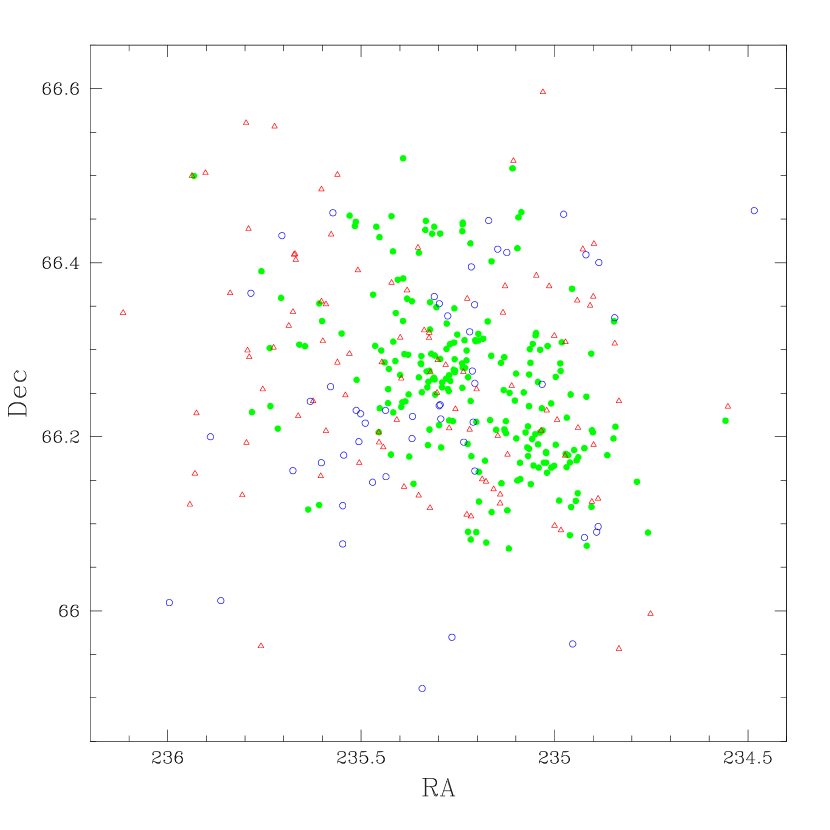
Figure 1: Coded positions of all galaxies in the spectroscopic database. Cluster members are represented by filled green circles, background galaxies by open red triangles, and foreground galaxies by open blue circles. The relative uniformity of sampling is indicated by the fairly even distribution of background galaxies.

With spectroscopy data coming from four separate sources, it is useful to investigate possible bias in our sampling of cluster galaxies (e.g., obtaining relatively more velocities for some portions of the cluster than for others). Fortunately, this is mitigated by the large (60′ diameter) field of view of WIYN+Hydra which equates to nearly 7 Mpc at the redshift of the cluster. In Figure 1 we plot the positions of all galaxies for which we have spectra. It can be seen that our spatial sampling is relatively uniform, particularly by noting the distribution of background galaxies (open triangles in the figure). Optical images of the cluster, particularly those with high resolution, often reveal tight groupings of galaxies (Owen et al., 2004). Limitations on fiber spacing with Hydra (37″) mean that any single fiber configuration will miss some galaxies. However, since seven different fiber configurations were observed (four in 1996, three in 2000) this effect is lessened. Overall, the net effect of missing a few galaxies in tight groupings should be minimal in performing the dynamical assessments. In fact, missing spectra for some galaxies in tight groups would result in less pronounced evidence for substructure than is actually present.

3 Analysis: Tests of Substructure

A histogram of the velocity data is presented in Figure 2. A2125 is easily seen as the single strong peak in the velocity distribution. In all, there are 224 cluster galaxies as identified via 3$\sigma$ clipping of the velocity data (Yahill & Vidal, 1977). The calculated biweight location and scale (see Beers, Flynn, & Gebhardt, 1990) are $73897\pm 74$ km s^-1 ($z=0.2465$) and $1113^{+57}_{-49}$ km s^-1, respectively. These numbers have been corrected for measurement errors (see Danese, de Zotti, & di Tullio, 1980), and the dispersion was calculated from relativistically-corrected velocities (which we use for all subsequent dynamics calculations). We adopt the biweight location as our cluster systemic velocity and the biweight scale as our cluster velocity dispersion for the remainder of this discussion. Note that the “non-robust” calculations of the mean and dispersion yield $73995\pm 96$ km s^-1 and $1150^{+59}_{-51}$ km s^-1, similar to the robust quantities.

The 224 cluster galaxies were subjected to a battery of statistical tests to evaluate potential substructure. These included tests performed exclusively on the velocity data (the “ROSTAT” package of Beers, Flynn, & Gebhardt, 1990), and tests on the galaxy positional data both with and without velocity information (for a complete listing and description of all tests, see Pinkney et al., 1996, hereafter PRBB). The advantages to using a battery of statistical tests are noted in PRBB. Essentially, each test provides a different perspective on the dynamical state of the cluster and taken collectively they often complement one another. Understanding a set of results is aided greatly by comparison with numerous N-body simulations.

The tests performed exclusively on the velocity data (“1D” tests) generally compare the distribution to that of a Gaussian, and are presented in Table 4. Since the computational algorithms in the ROSTAT package which are used to determine the significance for the $B_{1}$ and $B_{2}$ statistics ($B_{1}$ and $B_{2}$ are the canonical estimators of skewness and kurtosis, and represent the third and fourth moments of the velocity distribution) fail for large $N$, we have estimated their significance via 40 randomly-drawn subsets (with $N=150$) of the full data set. Most of the 1D tests indicated significant non-Gaussian behavior of the velocity histogram. Qualitatively, this may be understood by inspection of Figure 2. In particular, the cluster histogram has a “tail” at higher velocity. This produces significant skewness to the distribution, but does not make it overly kurtotic (e.g., the cluster distribution is more skewed than a Gaussian at better than $95\%$ confidence based on the $B_{1}$ statistic, yet consistent with a Gaussian in the sense of kurtosis based on the $B_{2}$ statistic). Consistent with the visual interpretation, combinations of the statistics indicate the distribution has more counts to the higher velocity side of the mean and similarly that the long tail identified by the tests resides on this side.

Similarly, tests performed on the positional data both with and without the associated velocities produced strong evidence for substructure. Table 5 presents the nine tests performed and their results. With the exceptions of the Angular Separation Test (West, Oemler, & Dekel, 1988) and the $\epsilon$ test (Bird, 1993), all indicate highly significant substructure (at $\geq 99.7\%$ confidence, as determined via 1000 Monte Carlo simulations). As an example, in Figure 3 we present the graphical representation of the $\Delta$ test (Dressler & Shectman, 1988). This test calculates local deviations from the systemic velocity ($v_{sys}$) and dispersion ($\sigma$) of the entire cluster:

$$\delta_{i}^{2}=\frac{N}{\sigma^{2}}\left[(v_{local}-v_{sys})^{2}+(\sigma_{local}-\sigma)^{2}\right].$$ (1)

Here $N$ is the number of galaxies which defines the local environment around galaxy $i$, taken to be $N=11$ in the original formulation of the test (i.e., a given galaxy and its ten nearest neighbors). For our calculations, we adopt $N=15$ (the square root of the total number of galaxies) as in PRBB. The sum of $\delta$ over all cluster members represents the actual test statistic, $\Delta$, and is approximately equal to the total number of cluster galaxies in the case of no substructure. Higher $\Delta$ indicate groupings which deviate from the cluster as a whole in either their mean velocity or dispersion (or both). For reference, $\Delta=309.9$ for our cluster sample of 224 galaxies. The significance is evaluated by Monte Carlo shuffles of the velocities while holding the positions fixed; this is the null hypothesis that there is no relationship between position and velocity. Graphically, each galaxy in the cluster may be represented by a circle with radius proportional to $e^{\delta_{i}}$. Thus, collections of larger circles indicate regions of substructure. Such regions are readily apparent in Figure 3, particularly to the northeast and southwest (and also slightly to the north of the cluster center).

In an attempt to identify substructures and determine which galaxies compose these substructures, we applied the KMM algorithm (see Ashman, Bird, & Zepf, 1994). This algorithm divides a system into a specified number of components and calculates the Gaussian distance (using both positions and velocities) of each galaxy to each component. The galaxies are assigned to their nearest component, new means and dispersions for the positions and velocities of each component are calculated, and the procedure is repeated. The algorithm converges when the assignments are stable. In addition to the assignments, the probability that a given assignment is accurate may be assessed through the Gaussian distances of that galaxy to each component. For example, if a galaxy were equidistant to two components its assignment would only imply $50\%$ confidence. It should be stressed that the algorithm is statistical and does not necessarily imply association with a real physical substructure. Any number of components may be specified by the user and the algorithm will attempt to apportion the data into those components. In some cases, the algorithm will either not converge or will remove nearly all galaxies from a given component, indicating the specified component is not viable.

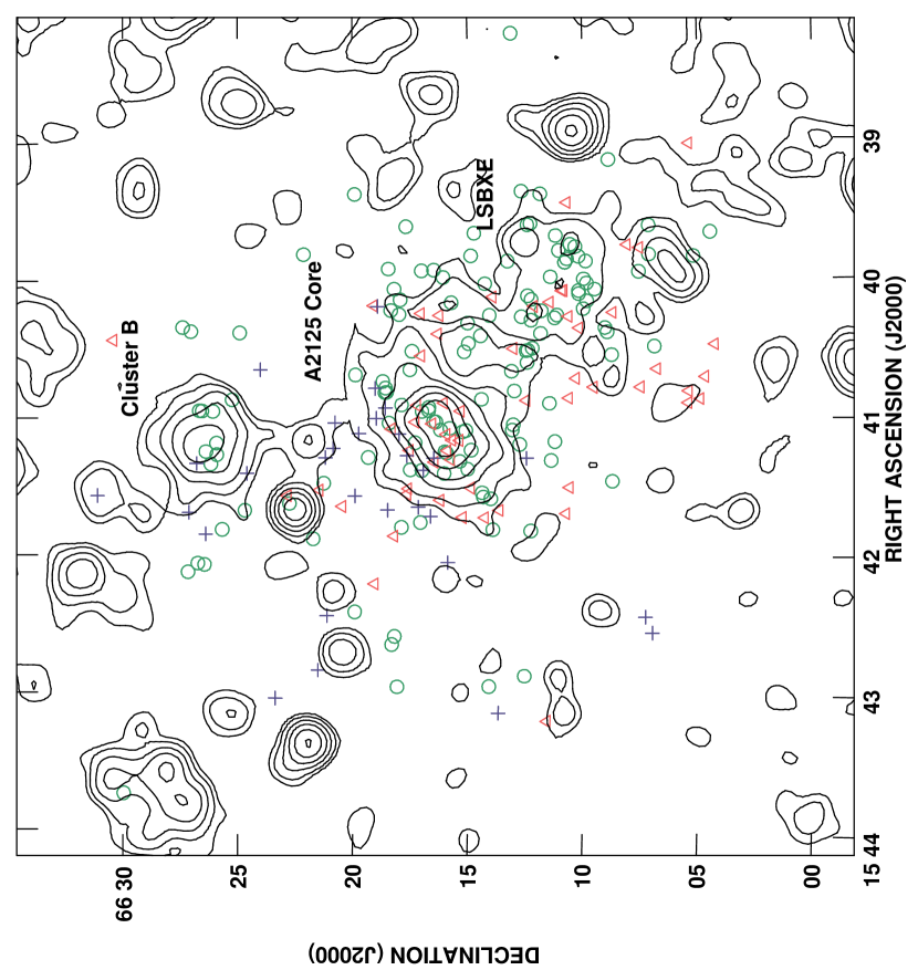
Figure 4: Distribution of Abell 2125 galaxies based on KMM fitting of three substructures, overlaid on X-ray contours from the smoothed ROSAT PSPC image. X-ray labels, as presented in Wang, Connolly, & Brunner (1997), are located above and to the right of the corresponding features. The red open triangles represent galaxies from the high velocity component, the blue pluses represent the low velocity component, and the green circles represent the main cluster (refer also to Figure 5 for the velocity histograms).

Based on the observation that the velocity histogram had a long tail at higher velocities, our first KMM run divided the cluster into two components, a primary and a higher velocity subcluster to the southwest. Noting the multiple regions for substructure in the graphical representation of the $\Delta$ test (Figure 3), we proceeded to a three-component fit. This fit kept the higher velocity subcluster to the southwest largely intact, and split off a lower velocity system to the northeast. This same general impression is obtained from an adaptively-smoothed distribution of the galaxy surface density, as shown in Figure 5 of Owen et al. (1999). Details of these KMM runs are provided in Tables 6 and 7, and the results of the three-component fit are depicted in Figures 4 and 5.

A slight digression on the validity of the KMM assignments is in order. The original astronomical application of KMM by Ashman, Bird, & Zepf (1994) was to detect bimodality in univariate datasets. For this purpose, and assuming the data are split into two components of equal dispersion but different mean, the authors found KMM to be relatively insensitive to input parameters. As might be expected, we have found through extensive testing that addition of variables largely removes this independence on input conditions. Clearly, adding two additional variables (for position) and relaxing the constraint that different components have common dispersions in a given variable expands the set of possible solutions. For example, with carefully chosen input parameters we were able to produce a two-component fit which largely ignored velocity and separated the cluster into a main component and a southwest clump, and a three-component fit which largely ignored position and sub-divided the higher velocity galaxies into two components. The merits of these various solutions are difficult to debate; Ashman, Bird, & Zepf (1994) note that the significance at which an additional substructure improves the fit to the data is difficult to determine in all but the fairly simple case of a single variable decomposed into two components of equal dispersion but different mean. It is largely for these reasons that we did not extend the KMM analysis to more than three components. We note here that other solutions exist, but the two we discuss were driven by the substructure test results and in particular by the locations of substructure indicated by the $\Delta$ test (Figure 3).

The KMM assignments enable us to revisit Figure 3, the Dressler-Shectman bubble plot (refer also to Figure 4). Three regions of possible substructure are identified from the plot as collections of larger circles: one to the northeast, one to the southwest, and one slightly north of the cluster core. These may be caused either by groupings of galaxies at a velocity differing from the cluster as a whole, or by groupings of galaxies with local dispersions differing from the cluster as a whole (refer to Equation 1). The possible northeast substructure has larger $\delta$ values primarily because its galaxies are at a lower velocity than the cluster. This corresponds to the lower velocity component identified in the KMM runs fitting more than two substructures. The possible southwest substructure has larger $\delta$ values both because: 1) its galaxies have a higher local systemic velocity than the remainder of the cluster, and 2) the higher velocity galaxies are seen in projection with galaxies at the same general velocity as the cluster, thus increasing the velocity dispersion among nearest neighbors (in particular, note the concentration of higher velocity galaxies to the southeast of the main southwest clump). This region corresponds to the higher velocity component identified in the KMM runs. Finally, the higher local $\delta$ values just to the north of the cluster core are the result of large local velocity dispersion. This is caused by the superposition of galaxies from the low velocity substructure, the high velocity substructure, and the main body of the cluster.

4 Discussion

4.1 The Dynamical State of A2125

The above analysis indicates that A2125 possesses very strong evidence for substructure. What is the cause of this behavior? There are several possible interpretations. It is possible that we are simply viewing a projection of multiple clusters. The velocity separation of the main cluster and the higher velocity system implies a physical separation of $\sim$45 Mpc, assuming the difference is simply due to the Hubble flow. Their close alignment along the line of sight would then be fairly remarkable. Bahcall et al. (2003) used early Sloan Digital Sky Survey data to compile a cluster catalog out to $z\sim 0.3$, and from these data determined an estimate of the space density of galaxy clusters. Should clusters be distributed randomly, this space density implies that the probability of any two clusters being seen at an angular separation of less than or equal to that implied by the KMM fits is 2.2$\%$. If we restrict this further to clusters at the redshifts implied by the KMM fits, the probability is only 0.1$\%$. Of course, this is a gross estimate; it ignores the reality of large-scale structure (which would increase the probability of such an alignment) but also does not take into account the richness of the clusters (the SDSS catalog includes substantially poorer clusters, so the chance of two clusters as rich as implied by the velocity dispersions in Table 6 being aligned would be lower). In addition, a simple superposition does not entirely fit with the X-ray data. Figure 4 includes X-ray contours derived from the smoothed ROSAT data. The cluster galaxies reported in this study match reasonably well with the X-ray features, with concentrations tracing the core of A2125 and the more diffuse X-ray emission to the southwest (labelled “LSBXE” after Wang, Connolly, & Brunner (1997)). Although there is substantial overlap in the positional distributions of galaxies in the KMM fits, a rough mapping has the higher velocity system associated with the southwest X-ray emission. But as noted in Wang, Connolly, & Brunner (1997) and Wang, Owen, & Ledlow (2004), this region is not simply explained as a single cluster or group: it is too diffuse to be a virialized cluster (and is composed primarily of spiral galaxies), and although its X-ray temperature ($\sim$1 keV) is representative of groups its luminosity (over $10^{43}$ ergs s^-1) is in excess of typical group luminosities by an order of magnitude. Our velocity data also indicate a much higher dispersion than would be expected for a single poor cluster or group, and similarly that the velocities are poorly fit by a Gaussian (Figure 5, although the Gaussian hypothesis for this component can not be rejected via either the $I$ or $KS$ tests). Thus, these X-ray papers favor that the diffuse X-ray emission to the southwest arises from hot intergalactic gas in a hierarchical structure including multiple groups. Presumably, this structure is oriented roughly along our line of sight and connects to the core of A2125.

Another possibility is that we are witnessing a cluster-cluster merger. This interpretation is based largely on comparison of the substructure test results with the N-body simulations of cluster-cluster mergers presented by PRBB. In general, the one-dimensional tests (i.e., those performed using only the galaxy velocities) are excellent indicators of mergers viewed near core passage when the relative velocity between the merging partners is greatest. Of course, this requires that the merger not be viewed orthogonal to the merger axis. Conversely, the 2D (positions only) tests perform best at early epochs of mergers and when the system is viewed orthogonal to the merger axis, thereby maximizing the positional separation of the merging partners. The 3D tests combine the strengths and weaknesses of their lower dimensional counterparts.

Such consistently strong indications of substructure as are found in A2125 (refer to Table 5) are fairly rare in the simulations. Even so, the results are generally consistent with either of two possibilities. The first is the earlier stages of a merger (up to 2 Gyr prior to core passage) in which the positional separation of the two components is large, and consequently the system is viewed closer to orthogonal to the merger axis. The second possibility is a merger seen near the epoch when the cores of the respective clusters have become coincident and with a viewing angle more closely aligned with the merger axis (within about 30^∘). Since this latter possibility is the same as that obtained from the 1D substructure tests, this scenario best matches the A2125 data. It is also interesting to note that the two multi-dimensional tests which do not suggest overly strong evidence for a merger are the two least sensitive tests identified by the simulations. These are the Angular Separation Test (AST; West, Oemler, & Dekel, 1988) and the $\epsilon$ test (Bird, 1993). The AST looks for substructure in the form of small angular separations where the angle between any two galaxies is defined using the cluster centroid as the vertex. It therefore performs best when subclusters are well separated, a condition that fails around the time of core passage or if the system is viewed along the merger axis. The $\epsilon$ test calculates the projected mass estimator in the vicinity of galaxies using their nearest neighbors. Regions of substructure have lower projected mass estimates than the global mass estimate, and the significance of this deviation is tested via Monte Carlo shuffles of the data. Although the $\epsilon$ test is sensitive to mergers, it is most sensitive for times well after core passage (PRBB).

If the merger hypothesis is correct, whether the system is being viewed before or after core passage is dependent on the viability of the lower velocity component in the KMM fits. PRBB note that the difference in the velocity dispersions of the two components (for ease of reference, hereafter called the primary and the subcluster) is a good diagnostic of the timing of the merger (see their Table 9). Prior to core passage, the velocity dispersion of the primary is larger than that of the subcluster simply because of its greater mass. As the subcluster merges with the primary, it is dispersed and thereby obtains the larger dispersion. In the two-component KMM fit, the subcluster has a slightly lower velocity dispersion and would then indicates that the system is being viewed shortly before core passage (see Table 6). Removing the lower velocity galaxies from the primary when going to a three-component fit reduces the dispersion of the primary below that of the subcluster, suggesting the system is viewed shortly after core passage. In either case the high relative velocity of subcluster to the primary, $1940$ km s^-1 in the two-component fit and $1702$ km s^-1 in the three-component fit, is consistent with viewing a merger near the time of core passage (e.g., see Equation 15 and associated discussion in Sarazin, 2002).

A simple sanity check on the merger hypothesis is to ask whether the presumed merging parties are bound. Treating the primary and subcluster as point masses, the simple Newtonian condition for a bound system is:

$$V_{r}^{2}R_{p}\leq 2GM\mbox{sin}^{2}\alpha~{}\mbox{cos}~{}\alpha$$ (2)

where $V_{r}$ is the line of sight velocity difference between the two masses, $R_{p}$ is their projected separation, $M$ is the total mass, and $\alpha$ is the projection angle defined from the plane of the sky. The KMM analysis provides a reference from which to evaluate this condition, in particular by providing estimates for $V_{r}$, $R_{p}$, and $M$ (under the assumption that each the primary and the subcluster represent virialized systems). In the two-component fit, $V_{r}=1940$ km s^-1, $R_{p}=700$ kpc, and $M=3.4\times 10^{15}$ M_⊙ (the virial mass for the primary and subcluster are $2.1\times 10^{15}$ and $1.3\times 10^{15}$, respectively). Thus, the system is bound for nearly all projection angles ($6^{\circ}\leq\alpha\leq 84^{\circ}$). Only if the total mass of the system is very low ($\lesssim 8\times 10^{14}$ M_⊙) would the system be unbound. Similarly, using the two largest components in the three-component fit the system would be bound for $5^{\circ}\leq\alpha\leq 85^{\circ}$ and unbound if $M\lesssim 5\times 10^{14}$ M_⊙. Note that in this latter case, the virial assumption is surely suspect as the subcluster has the larger velocity dispersion and hence implied mass ($0.9\times 10^{15}$ M_⊙ for the primary and $1.4\times 10^{15}$ M_⊙ for the subcluster).

This merger hypothesis is potentially further supported by the X-ray morphology, although as with the case of a simple superposition there are difficulties. The X-ray emission of the main body of A2125 is elongated in a direction perpendicular to the low surface brightness X-ray emission. This elongation is consistent with “an initial coalescence of subunits of comparable masses” (Wang, Connolly, & Brunner, 1997), whereas at later stages the elongation would tend to be along the supercluster filament (see also the simulations of Roettiger, Loken, & Burns, 1997). However, it is clear that the X-ray emission from the main body of A2125 represents only a small portion of the entire system (refer to Figure 4). While a merger of some sort is indicated by the X-ray data, the scale of this merger is debatable.

In any case, we are observing A2125 under special circumstances which may largely explain some of the peculiarities of the cluster. At Richness Class 4, it is among the very richest clusters of galaxies known (e.g., Morrison et al., 2003). Similarly, its large velocity dispersion suggests that it is a massive cluster containing many galaxies. However, these factors are inconsistent with the low X-ray luminosity and temperature of the cluster ($L_{X}=7.9\times 10^{43}$ ergs s^-1 and $T=3.2$ keV; Wang, Owen, & Ledlow, 2004). For example, using the $\sigma-T$ relationship of Lubin & Bahcall (1993) the velocity dispersion of A2125 would predict a temperature of 7.5 keV. Such a discrepancy can be explained if the system is composed of multiple complexes seen in projection, whether these components are merging or not. A more appropriate application of the $\sigma-T$ relationship would then be for an individual cluster in the system. Working backwards, the X-ray temperature predicts a velocity dispersion of about 670 km s^-1, a figure in line with the velocity dispersions of the larger substructures (i.e., components with the most members) identified in the KMM analysis (refer to Table 6).

4.2 Emission Line vs. Non-Emission Line Galaxies

As prior studies (e.g., Owen et al., 1999; Morrison et al., 2003) have noted an excess in the fraction of active galaxies in A2125 relative to other clusters of comparable richness, we performed a simple investigation of activity as defined by presence of emission lines. For this purpose, the noted presence of any emission line in a galaxy’s spectrum regardless of the strength of that line was sufficient for inclusion of that galaxy in the emission line sample. Using this definition, 75 of 224 cluster galaxies ($33.5\%$) were emission line objects. Unfortunately, we lack comparable data sets for other intermediate-redshift clusters to test whether this fraction is unusually high. For comparison, 96 of the 151 non-cluster galaxies in the field of A2125 ($63.6\%$) were emission line objects.

When measured over the entire cluster, the dynamics of the emission line galaxies do not differ significantly from those of the non-emission line galaxies. The systemic velocity and dispersion for the emission line galaxies were $73798\pm 133$ km s^-1 and 1148${}^{+107}_{-84}$ km s^-1, respectively, while those for the non-emission line galaxies were $73950\pm 90$ km s^-1 and $1092^{+70}_{-58}$ km s^-1. Similarly, there is no significant evidence that the emission line galaxies are drawn from a different population than the cluster galaxies as a whole, as quantified by KS and Wilcoxon tests. The positional data suggest that the emission line galaxies are at lower declinations, although this is significant only at 1.85$\sigma$. We also checked whether the emission line galaxies were preferentially associated with any substructures identified via the KMM analysis. A $\chi^{2}$ test indicated that there was no statistical difference in the fraction of galaxies with emission lines among the various groups. Thus, the emission line galaxies are fairly well mixed throughout the cluster.

5 Conclusions

We have reported on a program which has obtained 371 galaxy velocities in the direction of the $z=0.2465$ rich cluster Abell 2125. These new velocities include 222 cluster galaxies (including 25 in common with those reported in Owen et al. (1999)) which increases the total number of confirmed cluster members to 224, making this among the better studied intermediate redshift Butcher-Oemler clusters. The galaxy velocities were subjected to a large number of statistical tests which identified significant substructure. Through comparison with numerical simulations, these tests indicated that A2125 is consistent with a merger of comparable-mass clusters viewed along an axis within $\sim 30$^∘ of the merger axis. This merger is viewed within a few hundred million years of the time at which the cores of the respective components have crossed.

A favorable alignment of multiple structures, be they involved in a merger or simply seen in projection, is helpful in understanding the general properties of A2125. The combination of these structures produces an unusually high richness and velocity dispersion, reconciling the apparent discrepancy of the richness of the cluster with its low X-ray temperature and luminosity.

Table 1: Summary of Observations

Field ID	Date	Exposures	Instrument
H1	1996 April 16	$6\times 1800$	WIYN+Hydra
H2	1996 April 16	$2\times 2400$	WIYN+Hydra
	1996 April 17	$4\times 2400$	WIYN+Hydra
H3	1996 April 17	$3\times 2580$	WIYN+Hydra
	1996 April 18	$4\times 2580$	WIYN+Hydra
H4	1996 May 20	$4\times 2100$	WIYN+Hydra
	1996 May 21	$2\times 2100$	WIYN+Hydra
	1996 May 22	$2\times 2100$	WIYN+Hydra
1187	1998 May 27	$2\times 1800$	Mayall multislits
1188	1998 May 27	$2\times 1800$	Mayall multislits
1189	1998 May 27	$2\times 1800$	Mayall multislits
1191	1998 May 27	$2\times 1800$	Mayall multislits
1196	1998 May 28	$2\times 1800$	Mayall multislits
1197	1998 May 28	$2\times 1800$	Mayall multislits
1198	1998 May 28	$2\times 1800$	Mayall multislits
1199	1998 May 28	$2\times 1800$	Mayall multislits
1200	1998 May 28	$2\times 1800$	Mayall multislits
1190	1998 May 29	$2\times 1800$	Mayall multislits
1192	1998 May 29	$2\times 1800$	Mayall multislits
1193	1998 May 29	$2\times 1800$	Mayall multislits
1194	1998 May 29	$2\times 1800$	Mayall multislits
Q101	2000 March 30	$4\times 2800$	WIYN+Hydra (queue)
	2000 April 2	$2\times 2800$	WIYN+Hydra (queue)
Q102	2000 May 27	$6\times 2800$	WIYN+Hydra (queue)
Q103	2000 May 28	$5\times 2800$	WIYN+Hydra (queue)

Note. — Exposure times are in seconds.

Table 2: Cluster Velocity Data

RA	Dec	$cz$	Error	Lines	Source
15 38 13.9	+66 13 06	74199	81	$\cdots$	W00
15 39 02.0	+66 05 24	77196	81	$\cdots$	W00
15 39 08.8	+66 08 54	73449	49	$\cdots$	W00
15 39 22.2	+66 12 42	73419	40	[O ii], [O iii]	W00
15 39 23.1	+66 19 58	73068	40	[O ii], H $\beta$	W96
15 39 23.5	+66 11 53	73226	81	$\cdots$	W96
15 39 27.3	+66 10 44	76660	67	$\cdots$	W96
15 39 36.4	+66 12 19	73676	88	([O ii])	W96
15 39 36.8	+66 12 27	73387	59	$\cdots$	W96
		73359	51	$\cdots$	W00
15 39 37.2	+66 07 10	72738	63	$\cdots$	W96
15 39 37.3	+66 17 44	73047	51	$\cdots$	W96
15 39 40.1	+66 04 29	73989	40	[O ii], H $\beta$, [O iii], H $\alpha$, [N ii]	W00
15 39 40.3	+66 14 46	74431	66	$\cdots$	W96
15 39 41.5	+66 11 13	72672	54	$\cdots$	W96
15 39 45.4	+66 10 35	72602	63	$\cdots$	W96
		72460	49	$\cdots$	M98
15 39 45.7	+66 08 06	74791	70	$\cdots$	W96
15 39 46.4	+66 10 22	72622	57	$\cdots$	W96
		72700	57	$\cdots$	M98
15 39 46.9	+66 07 34	75098	57	$\cdots$	W96
15 39 48.0	+66 11 05	72248	52	$\cdots$	W96
		72250	49	$\cdots$	M98
15 39 49.2	+66 22 12	73871	40	[O ii], H $\beta$, [O iii]	W96
15 39 49.7	+66 07 09	73446	40	H $\alpha$, [N ii]	W00
15 39 50.1	+66 14 55	73621	61	$\cdots$	W96
15 39 50.5	+66 05 13	73189	40	[O ii], H $\beta$	W96
15 39 50.5	+66 10 13	72666	59	$\cdots$	W96
15 39 51.6	+66 10 44	72190	40	H $\beta$, H $\alpha$, [N ii]	M98
15 39 52.5	+66 13 19	74408	40	H $\alpha$, [N ii]	W00
15 39 52.6	+66 09 54	73648	54	$\cdots$	W96
		73689	46	$\cdots$	W00
15 39 53.0	+66 10 48	73546	51	$\cdots$	W96
		73749	57	$\cdots$	M98
		73389	57	$\cdots$	M98
15 39 55.6	+66 18 30	73492	52	$\cdots$	W96
15 39 56.2	+66 16 32	72787	59	$\cdots$	W96
15 39 56.4	+66 17 04	73908	62	$\cdots$	W96
15 39 57.2	+66 07 36	73493	62	$\cdots$	W96
15 39 59.3	+66 11 27	73796	40	[O ii], H $\beta$, [O iii]	W96
		73734	40	[O ii], H $\beta$, [O iii], H $\alpha$, [N ii]	M98
15 39 59.4	+66 16 08	73684	55	$\cdots$	W96
15 40 00.3	+66 10 00	73479	61	$\cdots$	M98
15 40 02.0	+66 09 53	72640	40	[O ii], H $\alpha$, [N ii]	M98
15 40 02.2	+66 14 18	73809	40	H $\alpha$, [N ii]	W00
15 40 04.3	+66 18 16	74662	54	$\cdots$	W96
15 40 04.7	+66 09 31	73929	61	$\cdots$	M98
15 40 05.2	+66 10 53	75638	57	$\cdots$	M98
15 40 05.3	+66 10 56	75818	52	$\cdots$	W96
		75757	51	$\cdots$	M98
15 40 05.4	+66 10 13	72619	51	$\cdots$	W96
		72700	49	$\cdots$	W00
		72550	47	$\cdots$	M98
15 40 06.6	+66 10 13	73029	40	[O ii], H $\beta$, [O iii], H $\alpha$, [N ii]	W00
15 40 07.5	+66 12 26	74105	55	$\cdots$	W96
		74049	49	$\cdots$	M98
15 40 07.9	+66 13 57	77091	62	$\cdots$	W96
15 40 09.0	+66 17 59	73760	62	$\cdots$	W96
15 40 09.0	+66 12 17	73585	53	$\cdots$	W96
		73509	49	$\cdots$	M98
15 40 09.8	+66 09 52	73734	78	$\cdots$	W96
		73999	57	$\cdots$	M98
15 40 10.3	+66 11 29	76890	50	$\cdots$	W96
		76657	51	$\cdots$	M98
15 40 10.4	+66 15 46	74170	55	$\cdots$	W96
15 40 11.5	+66 19 09	77075	60	$\cdots$	W96
15 40 11.8	+66 18 59	71811	53	$\cdots$	W96
15 40 12.0	+66 12 10	76700	51	$\cdots$	W96
		76627	49	$\cdots$	W00
15 40 13.1	+66 10 01	73749	40	[O ii], H $\beta$, [O iii], H $\alpha$	M98
15 40 13.6	+66 18 24	74746	49	$\cdots$	W96
15 40 13.9	+66 11 50	73750	40	[O ii], H $\beta$, [O iii]	W96
		73689	40	[O ii], H $\beta$, [O iii], H $\alpha$, [N ii]	W00
15 40 14.8	+66 08 44	75849	74	$\cdots$	W96
15 40 15.0	+66 17 06	75334	66	$\cdots$	W96
15 40 15.4	+66 18 03	72904	40	[O ii], H $\beta$, [O iii]	W96
		72939	40	[O ii], H $\gamma$, H $\beta$, [O iii], H $\alpha$, [N ii]	W00
15 40 15.8	+66 16 17	75301	52	$\cdots$	W96
15 40 15.8	+66 14 07	74588	61	$\cdots$	W00
15 40 15.9	+66 11 10	73591	40	[O ii], H $\beta$, [O iii]	W96
		73839	40	H $\beta$, [O iii], H $\alpha$, [N ii]	M98
15 40 16.5	+66 10 40	76619	51	$\cdots$	W96
		76537	51	$\cdots$	M98
15 40 16.5	+66 12 43	73002	48	$\cdots$	W96
		72640	61	$\cdots$	M98
15 40 17.1	+66 11 16	73255	70	([O ii], H $\beta$)	W96
		73209	40	[O ii], H $\alpha$	M98
15 40 18.1	+66 12 18	74558	61	$\cdots$	M98
15 40 19.2	+66 15 03	73722	51	$\cdots$	W96
15 40 20.6	+66 27 29	73253	72	$\cdots$	W96
15 40 21.3	+66 09 04	73752	60	$\cdots$	W96
15 40 21.4	+66 10 12	76813	49	$\cdots$	W96
		76897	46	$\cdots$	W00
15 40 22.3	+66 27 07	74449	76	$\cdots$	W96
15 40 23.1	+66 25 00	74044	56	$\cdots$	W96
15 40 23.2	+66 08 58	73921	51	$\cdots$	W96
15 40 23.8	+66 11 53	72999	57	$\cdots$	M98
15 40 23.9	+66 16 21	74954	51	$\cdots$	W96
15 40 24.7	+66 14 30	73149	69	$\cdots$	W00
15 40 28.0	+66 15 02	74199	40	[O ii], H $\beta$, [O iii], H $\alpha$, [N ii]	W00
15 40 28.4	+66 04 17	75487	65	$\cdots$	W96
15 40 29.4	+66 06 55	72491	50	$\cdots$	W96
		72580	47	$\cdots$	W00
15 40 30.1	+66 12 14	73578	40	[O ii], H $\beta$	W96
		73689	40	[O ii], H $\beta$, [O iii], H $\alpha$, [N ii]	M98
15 40 30.3	+66 13 04	74758	49	$\cdots$	W96
		74888	61	$\cdots$	M98
15 40 30.9	+66 12 26	74169	40	[O ii], H $\alpha$	M98
15 40 31.3	+66 12 31	74198	40	[O ii], [O iii]	W96
15 40 31.3	+66 17 29	72790	56	$\cdots$	W96
		72819	49	$\cdots$	W00
15 40 31.5	+66 15 13	73269	40	[O ii], H $\beta$, [O iii], H $\alpha$	W00
15 40 33.0	+66 08 47	72794	54	([O ii])	W96
		72879	49	$\cdots$	W00
15 40 33.3	+66 17 06	76255	51	$\cdots$	W96
		76447	49	$\cdots$	W00
15 40 36.4	+66 12 28	72640	40	H $\beta$, H $\alpha$, [N ii]	W00
15 40 39.1	+66 06 48	76541	40	[O ii], H $\beta$, [O iii]	W96
15 40 39.1	+66 24 06	71380	40	[O ii], H $\beta$, [O iii], H $\alpha$, [N ii]	W00
15 40 39.3	+66 17 35	74542	74	$\cdots$	W96
15 40 40.1	+66 13 09	73724	40	[O ii], H $\beta$, [O iii]	W96
		73718	40	[O ii], H $\gamma$, H $\beta$, [O iii], H $\alpha$, [N ii], [S ii]	M98
15 40 41.5	+66 19 57	72884	73	$\cdots$	W96
		72819	40	H $\beta$, H $\alpha$, [N ii]	W00
15 40 42.4	+66 04 42	75560	40	[O ii], H $\beta$	W96
		75578	40	[O ii], H $\alpha$, [N ii]	W00
15 40 43.2	+66 10 21	76687	40	[O ii], H $\beta$, H $\alpha$, [N ii]	W00
15 40 44.3	+66 18 46	73059	57	$\cdots$	W00
		73419	81	$\cdots$	M98
15 40 47.0	+66 07 31	76841	40	[O ii], H $\beta$	W96
15 40 47.0	+66 09 34	75216	84	([O ii], H $\beta$)	W96
15 40 47.2	+66 18 38	73079	52	$\cdots$	W96
		73149	49	$\cdots$	M98
15 40 47.3	+66 19 06	71974	51	$\cdots$	W96
		72340	61	$\cdots$	M98
15 40 48.5	+66 13 02	72640	53	$\cdots$	W00
15 40 48.6	+66 05 25	76761	52	$\cdots$	W96
15 40 49.0	+66 18 36	73299	61	$\cdots$	M98
15 40 49.2	+66 18 40	72972	54	$\cdots$	W96
		73059	57	$\cdots$	M98
15 40 51.8	+66 10 39	75337	56	$\cdots$	W96
15 40 52.0	+66 04 55	75092	73	([O ii], H $\beta$)	W96
15 40 52.2	+66 14 28	72518	40	[O ii], H $\beta$, [O iii]	W96
		72670	40	[O ii], [O iii], H $\alpha$, [N ii]	M98
15 40 52.2	+66 25 20	74409	59	$\cdots$	W96
15 40 52.7	+66 12 31	77551	40	[O ii], H $\beta$	W96
		77586	40	[O ii], H $\beta$, H $\alpha$	W00
15 40 53.6	+66 05 26	75147	66	([O ii])	W96
		75188	40	[O ii], H $\alpha$, [N ii]	W00
15 40 53.7	+66 16 07	76297	61	$\cdots$	W00
15 40 54.5	+66 11 28	74468	40	[O ii], H $\beta$, H $\alpha$, [N ii]	M98
15 40 54.6	+66 17 57	72727	52	$\cdots$	W96
		72819	51	$\cdots$	M98
15 40 54.7	+66 17 16	76819	58	$\cdots$	W96
		76777	40	[O ii], H $\beta$, H $\alpha$, [N ii]	W00
		76747	40	[O ii], H $\alpha$, [N ii]	M98
15 40 55.6	+66 16 45	74528	61	$\cdots$	M98
15 40 55.9	+66 18 39	72280	61	$\cdots$	M98
15 40 56.9	+66 26 46	73787	62	$\cdots$	W96
		73929	49	$\cdots$	W00
15 40 57.0	+66 16 46	74217	58	$\cdots$	W96
15 40 57.0	+66 26 39	73329	67	$\cdots$	W96
15 40 57.2	+66 26 10	73437	57	$\cdots$	W96
15 40 57.3	+66 15 22	76297	40	H $\beta$, H $\alpha$	W00
15 40 57.4	+66 17 03	73620	51	$\cdots$	W96
		73749	49	$\cdots$	M98
15 41 0.3	+66 19 03	71686	51	$\cdots$	W96
		71800	45	$\cdots$	W00
15 41 01.7	+66 16 33	74079	57	$\cdots$	M98
15 41 01.9	+66 16 27	73679	49	$\cdots$	W96
		73659	46	$\cdots$	W00
		73629	51	$\cdots$	M98
15 41 02.0	+66 17 21	76479	70	$\cdots$	W96
		76957	69	$\cdots$	M98
15 41 02.3	+66 20 51	72062	57	$\cdots$	W96
15 41 02.4	+66 18 30	73569	40	[O ii], H $\beta$, [O iii], H $\alpha$, [N ii]	W00
		73749	40	[O ii], H $\alpha$	M98
15 41 02.6	+66 16 37	75098	69	$\cdots$	W00
15 41 03.2	+66 13 05	73037	56	$\cdots$	W96
15 41 04.7	+66 15 51	74225	65	$\cdots$	W96
		74199	61	$\cdots$	M98
15 41 05.0	+66 18 23	77047	40	[O ii], H $\beta$	M98
15 41 05.4	+66 16 15	73269	57	$\cdots$	M98
15 41 05.4	+66 13 07	72640	40	H $\beta$, [O iii], H $\alpha$	W00
15 41 05.7	+66 15 09	73197	40	[O ii], H $\beta$, [O iii]	W96
		73029	40	[O ii], H $\beta$, [O iii], H $\alpha$	M98
15 41 06.2	+66 15 17	73959	69	$\cdots$	W00
15 41 06.9	+66 19 49	72103	70	([O ii])	W96
15 41 07.0	+66 18 03	71770	81	$\cdots$	M98
15 41 07.4	+66 15 59	75098	61	$\cdots$	W00
15 41 09.8	+66 15 45	75846	58	([O ii], H $\beta$, [O iii])	W96
		75697	40	[O ii], [O iii], H $\alpha$, [N ii]	M98
15 41 09.9	+66 15 25	74768	61	$\cdots$	M98
15 41 10.5	+66 11 16	73496	59	$\cdots$	W96
15 41 10.9	+66 17 21	74376	54	$\cdots$	W96
		74408	61	$\cdots$	M98
15 41 11.0	+66 26 01	73843	89	$\cdots$	W96
15 41 11.7	+66 12 48	74139	40	[O ii], H $\beta$, H $\alpha$, [N ii]	W00
15 41 13.3	+66 20 56	71936	70	$\cdots$	W96
15 41 14.1	+66 14 55	73082	52	$\cdots$	W96
		73119	46	$\cdots$	W00
15 41 14.3	+66 17 36	75993	50	$\cdots$	W96
		76027	51	$\cdots$	M98
15 41 14.4	+66 15 57	75389	50	$\cdots$	W96
		75368	47	$\cdots$	W00
		75518	46	$\cdots$	M98
15 41 14.7	+66 26 28	74061	50	$\cdots$	W96
15 41 14.9	+66 16 04	73971	47	$\cdots$	W96
		73929	46	$\cdots$	M98
15 41 15.4	+66 15 59	73929	49	$\cdots$	W00
15 41 16.1	+66 26 00	73175	52	$\cdots$	W96
15 41 16.6	+66 17 43	72630	66	([O ii], H $\beta$)	W96
		72610	40	[O ii], H $\beta$, H $\alpha$, [N ii]	M98
15 41 17.3	+66 19 24	73899	51	$\cdots$	W00
15 41 17.3	+66 21 16	72154	54	$\cdots$	W96
15 41 17.6	+66 16 33	72536	53	$\cdots$	W96
		72370	61	$\cdots$	M98
15 41 17.7	+66 12 30	72408	40	[O ii], H $\beta$, [O iii]	W96
15 41 18.3	+66 15 47	75727	61	$\cdots$	M98
15 41 18.6	+66 11 25	74140	40	[O ii], H $\beta$	W96
15 41 19.0	+66 15 24	74348	49	$\cdots$	W00
15 41 19.3	+66 16 31	75836	52	$\cdots$	W96
		75697	51	$\cdots$	M98
15 41 19.9	+66 26 53	71511	58	$\cdots$	W96
15 41 20.2	+66 26 15	73434	51	$\cdots$	W96
15 41 22.4	+66 15 04	74502	73	$\cdots$	W96
15 41 22.7	+66 17 34	73899	61	$\cdots$	M98
15 41 22.8	+66 17 01	72216	40	[O ii], H $\beta$	W96
		72190	40	[O ii], H $\beta$, [O iii]	M98
15 41 23.0	+66 17 04	74434	84	$\cdots$	W96
15 41 24.2	+66 24 41	70742	57	$\cdots$	W96
15 41 24.2	+66 16 05	73538	68	$\cdots$	W96
		73599	47	$\cdots$	W00
15 41 27.6	+66 08 45	73536	50	$\cdots$	W96
15 41 28.5	+66 21 20	74468	40	[O ii], H $\beta$, [O iii], H $\alpha$, [N ii]	W00
15 41 30.3	+66 10 37	74841	40	[O ii], H $\beta$, [O iii]	W96
15 41 30.5	+66 14 55	75518	69	$\cdots$	W00
15 41 30.8	+66 17 40	75428	40	[O ii], H $\beta$, H $\alpha$, [N ii]	W00
15 41 31.5	+66 21 31	76300	53	$\cdots$	W96
15 41 32.6	+66 14 26	73729	52	$\cdots$	W96
15 41 33.2	+66 17 42	75188	40	[O ii], H $\alpha$	W00
15 41 33.9	+66 22 55	75368	61	$\cdots$	W00
15 41 33.9	+66 31 12	71021	61	$\cdots$	W00
15 41 34.0	+66 19 59	72613	52	$\cdots$	W96
15 41 34.4	+66 14 23	73459	52	$\cdots$	W96
15 41 35.1	+66 14 03	73689	69	$\cdots$	W00
15 41 35.9	+66 16 15	76027	61	$\cdots$	W00
15 41 37.3	+66 22 50	74588	40	[O ii], H $\beta$, H $\alpha$, [N ii]	W00
15 41 38.6	+66 20 32	74889	67	$\cdots$	W96
15 41 38.9	+66 17 13	71860	40	[O ii], H $\beta$, H $\alpha$, [N ii]	W00
15 41 40.1	+66 18 34	71436	60	$\cdots$	W96
15 41 40.1	+66 13 41	76177	40	[O ii], H $\beta$, H $\alpha$, [N ii]	W00
15 41 40.3	+66 24 46	73763	53	$\cdots$	W96
15 41 41.2	+66 27 12	71870	40	[O ii], H $\beta$	W96
15 41 41.5	+66 10 46	75458	57	$\cdots$	W00
15 41 42.8	+66 16 41	72123	52	$\cdots$	W96
15 41 43.2	+66 15 17	75383	58	$\cdots$	W96
15 41 43.4	+66 14 19	76447	62	$\cdots$	W96
15 41 45.5	+66 17 07	73537	57	([O ii])	W96
15 41 47.6	+66 17 57	74281	52	$\cdots$	W96
		74348	53	$\cdots$	W00
15 41 48.5	+66 13 58	73307	55	$\cdots$	W96
15 41 48.6	+66 25 46	74708	40	[O ii], H $\alpha$, [N ii]	W00
15 41 49.1	+66 12 18	74139	40	H $\alpha$, [N ii]	W00
15 41 50.6	+66 26 28	70606	62	$\cdots$	W96
15 41 51.3	+66 18 16	74749	59	$\cdots$	W96
15 41 52.7	+66 21 48	74503	40	[O ii], H $\beta$, [O iii]	W96
15 42 02.8	+66 15 55	72049	66	([O ii])	W96
		72310	40	H $\alpha$, [N ii]	W00
15 42 03.3	+66 26 49	74059	78	([O ii])	W96
		73989	40	H $\beta$, H $\alpha$, [N ii]	W00
15 42 03.9	+66 26 32	73680	40	[O ii], [O iii]	W96
15 42 07.1	+66 27 15	73815	60	$\cdots$	W96
15 42 12.1	+66 19 07	74998	40	[O ii], H $\beta$	W96
		74948	40	[O ii], H $\beta$, H $\alpha$	W00
15 42 24.3	+66 19 58	74109	53	$\cdots$	W00
		74139	61	$\cdots$	M98
15 42 26.0	+66 21 12	71614	49	$\cdots$	W96
15 42 26.1	+66 07 18	72206	40	[O ii], [O iii]	W96
15 42 32.9	+66 07 00	72275	40	[O ii], H $\beta$, [O iii]	W96
15 42 34.8	+66 18 15	74373	63	$\cdots$	W96
15 42 38.4	+66 18 22	74643	40	[O ii], H $\beta$, [O iii]	W96
15 42 49.7	+66 21 34	71752	51	([O ii])	W96
15 42 51.8	+66 12 34	73874	56	$\cdots$	W96
15 42 56.4	+66 14 07	74369	66	$\cdots$	W96
15 42 56.7	+66 18 07	74515	50	$\cdots$	W96
15 43 01.9	+66 23 25	71473	40	[O ii], H $\beta$, [O iii]	W96
15 43 07.8	+66 13 42	71856	40	[O ii], H $\beta$, [O iii]	W96
		71770	40	H $\beta$, [O iii], H $\alpha$, [N ii]	W00
15 43 11.1	+66 11 35	77295	40	[O ii], H $\beta$	W96

Note. — All coordinates are J2000, and heliocentric velocities (note that these are not relativistically corrected, and are therefore $cz$) and errors are in km s^-1. Emission lines used in determination of the reported velocities are indicated. When these are enclosed in parentheses, the velocity was determined through cross correlation but the noted emission lines were also detected at a consistent velocity. The abbreviations for the data sources are: W96 = WIYN Hydra 1996, W00 = WIYN Hydra 2000, and M98 = Mayall 1998.

Table 3: Non-cluster Redshifts

RA	Dec	$z$	Error	Lines	Source
15 37 56.1	+66 27 36	0.2049	0.0003	$\cdots$	W00
15 38 12.4	+66 14 05	0.4373	0.0001	[O ii], [O iii]	W00
15 39 00.4	+65 59 48	0.2878	0.0002	$\cdots$	W00
15 39 20.1	+66 14 28	0.3365	0.0003	$\cdots$	W00
15 39 20.1	+65 57 23	1.9010	0.0010	C iv, O iii], C iii]	W00
15 39 22.5	+66 18 26	2.2140	0.0010	C iv, C iii]	W00
15 39 22.7	+66 20 12	0.0231	0.0001	H $\beta$, [O iii], H $\alpha$, [S ii]	W96
15 39 32.5	+66 24 01	0.1210	0.0002	$\cdots$	W96
15 39 33.0	+66 05 48	0.0320	0.0001	H $\beta$, [O iii], H $\alpha$	W96
15 39 33.1	+66 07 44	0.4808	0.0002	$\cdots$	W00
15 39 34.0	+66 05 26	0.0323	0.0001	H $\beta$, [O iii], H $\alpha$, [N ii], [S ii]	W96
15 39 35.7	+66 25 18	0.3822	0.0001	[O ii], H $\beta$, [O iii]	W96
		0.3820	0.0001	[O ii], H $\gamma$, H $\beta$, [O iii], H $\alpha$, [N ii]	W00
15 39 35.8	+66 11 27	0.3612	0.0001	[O ii], H $\beta$, [O iii]	W00
15 39 36.1	+66 21 41	0.6776	0.0001	[O ii], H $\beta$	W00
15 39 36.9	+66 07 31	0.3224	0.0001	$\cdots$	W96
15 39 37.9	+66 21 03	0.4375	0.0001	[O ii], H $\beta$, [O iii]	W00
15 39 40.5	+66 24 33	0.1222	0.0002	$\cdots$	W96
15 39 41.5	+66 05 03	0.1228	0.0001	H $\beta$, [O iii], H $\alpha$	W96
15 39 42.5	+66 24 56	0.4078	0.0002	$\cdots$	W00
15 39 45.4	+66 12 37			$\cdots$	W00
15 39 46.4	+66 21 25	0.5226	0.0001	[O ii], H $\beta$, [O iii]	W00
15 39 48.8	+65 57 43	0.1225	0.0001	H $\beta$, [O iii], H $\alpha$, [S ii]	W00
15 39 53.3	+66 18 32	0.3718	0.0003	$\cdots$	W00
15 39 53.3	+66 10 42	0.6389	0.0001	[O ii], [O iii]	W00
15 39 54.3	+66 27 20	0.2031	0.0001	[O ii], H $\beta$, [O iii]	W96
15 39 56.1	+66 05 33	0.2755	0.0001	[O ii], H $\beta$	W96
		0.2759	0.0001	[O ii], H $\beta$	W00
15 39 58.4	+66 13 10	0.3411	0.0002	$\cdots$	W96
15 40 00.2	+66 18 58	0.2877	0.0001	[O ii], [O iii]	W00
15 40 03.4	+66 22 22	0.6760	0.0001	[O ii], H $\beta$	W00
15 40 04.8	+66 13 49	0.5465	0.0003	$\cdots$	W00
15 40 07.3	+66 35 46	0.2949	0.0002	$\cdots$	W00
15 40 07.7	+66 15 36	0.0930	0.0001	H $\beta$, [O iii], H $\alpha$	W96
15 40 08.5	+66 12 26	0.3223	0.0003	$\cdots$	W96
15 40 11.3	+66 23 07	0.3067	0.0003	$\cdots$	W00
15 40 25.4	+66 31 01	0.4401	0.0002	$\cdots$	W00
15 40 26.6	+66 15 30	0.3794	0.0001	[O ii], H $\beta$, H $\alpha$	W00
15 40 29.2	+66 10 47	0.3894	0.0001	[O ii], H $\gamma$, H $\beta$, [O iii]	M98
15 40 29.6	+66 24 42	0.0807	0.0001	H $\beta$, [O iii], H $\alpha$	W96
15 40 30.8	+66 22 24	0.3413	0.0001	[O ii], [O iii]	W96
15 40 32.0	+66 20 33	0.3622	0.0001	[O ii], [O iii]	W96
15 40 33.6	+66 08 02	0.9183	0.0001	Mg ii, [O ii]	W00
15 40 33.8	+66 07 25	0.2752	0.0001	[O ii], H $\beta$	W00
15 40 35.3	+66 12 05	0.2692	0.0001	$\cdots$	W00
15 40 35.3	+66 24 56	0.0808	0.0001	[O iii], H $\alpha$	W96
15 40 37.7	+66 08 24	0.6248	0.0002	$\cdots$	W00
15 40 40.8	+66 26 54	0.0563	0.0001	H $\alpha$, [N ii], [S ii]	W96
15 40 42.6	+66 08 54	0.6264	0.0003	$\cdots$	W00
15 40 44.9	+66 09 05			$\cdots$	W00
15 40 48.3	+66 15 17	0.3231	0.0001	[O ii], [O iii]	W96
15 40 49.5	+66 09 38	0.1964	0.0001	[O ii], [O iii]	W96
15 40 49.5	+66 15 41	0.1965	0.0003	$\cdots$	M98
15 40 49.6	+66 21 06	0.0683	0.0003	$\cdots$	W00
15 40 50.2	+66 25 53	0.9143	0.0010	Mg ii	W96
15 40 50.5	+66 13 00	0.2204	0.0003	$\cdots$	W00
15 40 51.0	+66 16 32	0.1270	0.0002	(H $\alpha$, [N ii])	W96
		0.1270	0.0001	H $\alpha$, [N ii], [S ii]	M98
15 40 51.7	+66 23 43	0.0376	0.0001	H $\beta$, [O iii], H $\alpha$, [S ii]	W96
15 40 51.9	+66 06 31	0.3632	0.0003	([O ii])	W96
		0.3657	0.0002	$\cdots$	W00
15 40 52.7	+66 19 14	0.1057	0.0001	H $\beta$, [O iii], H $\alpha$, [N ii], [S ii]	W96
		0.1059	0.0001	[O ii], H $\beta$, [O iii], H $\alpha$, [N ii], [S ii]	M98
15 40 54.3	+66 21 32	0.2957	0.0001	[O ii], H $\gamma$, H $\beta$, [O iii], H $\alpha$, [N ii], [S ii]	W00
15 40 54.6	+66 06 38	0.3605	0.0003	$\cdots$	W96
15 40 56.4	+66 11 38	0.0426	0.0001	H $\beta$, [O iii], H $\alpha$, [N ii], [S ii]	W96
15 40 56.4	+66 16 28	1.0120	0.0010	Mg ii, [O ii]	W00
15 41 00.8	+66 13 54	0.3614	0.0003	$\cdots$	W00
15 41 03.6	+65 58 11	0.1244	0.0001	H $\alpha$, [N ii], [S ii]	W00
15 41 05.3	+66 12 36	0.2749	0.0001	[O ii], H $\beta$, [O iii]	W96
		0.2752	0.0003	([O ii])	M98
15 41 06.3	+66 20 20	0.1094	0.0001	H $\beta$, [O iii], H $\alpha$, [N ii], [S ii]	W96
15 41 07.6	+66 16 57	0.2969	0.0003	$\cdots$	W00
15 41 10.6	+66 13 14	0.2270	0.0003	$\cdots$	M98
15 41 11.1	+66 14 13	0.0935	0.0001	H $\beta$, [O iii]	W96
15 41 11.5	+66 21 11	0.0863	0.0001	H $\beta$, [O iii], H $\alpha$, [N ii]	W96
15 41 11.6	+66 14 08	0.0932	0.0001	H $\beta$, [O iii], H $\alpha$, [N ii], [S ii]	W96
		0.0933	0.0001	H $\beta$, [O iii], H $\alpha$, [N ii], [S ii]	W00
15 41 12.5	+66 17 17	0.2704	0.0003	$\cdots$	W00
15 41 12.9	+66 15 02	0.5068	0.0003	$\cdots$	W00
15 41 14.6	+66 21 40	0.0855	0.0001	H $\alpha$, [N ii]	W96
		0.0854	0.0001	H $\gamma$, H $\beta$, [O iii], H $\alpha$, [N ii], [S ii]	W00
15 41 17.0	+66 16 27	0.6921	0.0003	([O ii])	W00
15 41 17.3	+66 07 06	0.3217	0.0003	$\cdots$	W00
15 41 17.8	+66 19 10	0.3344	0.0003	$\cdots$	M98
15 41 17.9	+66 18 49	0.3366	0.0003	$\cdots$	M98
15 41 20.9	+66 19 21	0.3597	0.0001	[O ii], H $\beta$	W00
15 41 22.1	+65 54 39	0.0783	0.0002	$\cdots$	W00
15 41 24.3	+66 07 57	0.3627	0.0001	[O ii], H $\beta$	W00
15 41 24.7	+66 25 02	0.3398	0.0001	[O ii], H $\beta$, [O iii]	W96
15 41 28.1	+66 13 25	0.0931	0.0001	H $\beta$, [O iii], H $\alpha$, [N ii], [S ii]	W96
15 41 28.6	+66 11 53	0.1265	0.0001	H $\beta$, [O iii], H $\alpha$	W96
15 41 31.5	+66 22 06	0.3395	0.0003	$\cdots$	W96
15 41 33.3	+66 08 33	0.3368	0.0003	$\cdots$	W00
15 41 35.1	+66 16 01	0.2752	0.0002	$\cdots$	W96
15 41 36.1	+66 18 50	0.3404	0.0001	[O ii], H $\beta$, [O iii]	W00
15 41 37.9	+66 13 10	0.5229	0.0001	[O ii], H $\gamma$, H $\beta$, [O iii]	W00
15 41 41.0	+66 22 38	1.3820	0.0010	C iii], Mg ii	W00
15 41 44.7	+66 09 15	0.1131	0.0002	$\cdots$	W96
15 41 44.9	+66 13 49	0.2113	0.0003	$\cdots$	W00
15 41 46.3	+66 11 16	0.5274	0.0002	$\cdots$	W00
15 41 47.3	+66 17 08	0.3220	0.0003	$\cdots$	W00
15 41 47.4	+66 11 25	0.5262	0.0003	$\cdots$	W00
15 41 48.9	+66 11 37	0.5263	0.0002	$\cdots$	W00
15 41 52.9	+66 08 52	0.1266	0.0001	H $\beta$, [O ii], H $\alpha$	W96
15 41 57.4	+66 12 56	0.2070	0.0001	[O ii], H $\beta$, [O iii]	W96
		0.2070	0.0001	[O ii], H $\gamma$, H $\beta$, [O iii], H $\alpha$, [N ii], [S ii]	W00
15 42 00.5	+66 13 36	0.1074	0.0001	H $\beta$, [O ii], H $\alpha$	W96
15 42 01.1	+66 10 12	0.5140	0.0002	$\cdots$	W00
15 42 01.5	+66 11 40	0.1459	0.0002	H $\beta$, [O iii]	W96
15 42 01.9	+66 23 30	0.4284	0.0001	[O ii], H $\gamma$, H $\beta$, [O iii]	W00
15 42 03.0	+66 13 49	0.1482	0.0003	([O iii])	W96
15 42 07.3	+66 17 44	0.3437	0.0001	[O ii], H $\beta$, [O iii]	W00
15 42 09.8	+66 14 52	0.3596	0.0001	[O ii], [O iii]	W00
15 42 10.8	+66 10 44	0.1091	0.0001	H $\beta$, [O iii], H $\alpha$	W96
15 42 11.4	+66 07 15	0.1266	0.0001	H $\beta$, [O iii], H $\alpha$	W96
15 42 11.4	+66 04 36	0.2248	0.0001	[O ii], H $\beta$, [O iii]	W96
		0.2248	0.0001	[O ii], H $\beta$, [O iii], H $\alpha$, [N ii]	W00
15 42 14.6	+66 30 04	0.2995	0.0002	([O ii])	W00
15 42 14.7	+66 17 08	0.5112	0.0001	[O ii], H $\gamma$, H $\beta$, [O iii]	W00
15 42 17.5	+66 27 26	0.1805	0.0001	[O ii], H $\beta$, [O iii]	W96
15 42 18.5	+66 25 56	0.2993	0.0001	[O ii], [O iii]	W96
15 42 18.9	+66 15 27	0.1463	0.0002	$\cdots$	W96
15 42 21.9	+66 12 24	0.2702	0.0001	[O ii], H $\beta$, [O iii]	W96
15 42 21.9	+66 21 08	0.3329	0.0001	[O ii], H $\beta$, [O iii]	W00
15 42 23.7	+66 18 36	0.3374	0.0002	$\cdots$	W00
15 42 24.6	+66 21 20	0.2972	0.0002	$\cdots$	W96
15 42 24.7	+66 10 12	0.2207	0.0001	[O ii], H $\beta$	W96
		0.2208	0.0001	[O iii], H $\alpha$, [N ii], [S ii]	W00
15 42 25.1	+66 09 17	0.6643	0.0001	[O ii], H $\beta$, [O iii]	W00
15 42 29.8	+66 14 28	0.5652	0.0001	[O ii], [O iii]	W00
15 42 31.6	+66 14 26	0.0928	0.0001	H $\beta$, [O iii], H $\alpha$, [N ii], [S ii]	W96
		0.0930	0.0001	H $\beta$, [O iii], H $\alpha$, [N ii], [S ii]	W00
15 42 39.2	+66 13 27	0.3607	0.0003	([O ii])	W96
		0.3612	0.0003	$\cdots$	W00
15 42 40.6	+66 24 12	0.2755	0.0001	[O ii], H $\beta$, [O iii]	W96
		0.2754	0.0001	[O ii], H $\beta$, [O iii], H $\alpha$, [N ii], [S ii]	W00
15 42 41.1	+66 24 37	0.2758	0.0001	[O ii], H $\beta$, [O iii]	W96
15 42 41.5	+66 24 34	0.2751	0.0001	[O ii], H $\gamma$, H $\beta$, [O iii], H $\alpha$, [N ii], [S ii]	W00
15 42 42.1	+66 20 36	0.6557	0.0001	[O ii], H $\beta$, [O iii]	W00
15 42 42.4	+66 09 40	0.0443	0.0001	H $\beta$, [O iii], H $\alpha$, [S ii]	W96
15 42 44.9	+66 19 39	0.3319	0.0002	$\cdots$	W96
15 42 49.1	+66 25 52	0.1469	0.0002	$\cdots$	W96
15 42 53.8	+66 33 23	0.3239	0.0001	[O ii], H $\beta$, [O iii], H $\alpha$	W00
15 42 54.4	+66 18 09	0.5082	0.0002	([O ii])	W00
15 43 01.1	+66 15 17	0.5113	0.0002	$\cdots$	W00
15 43 02.2	+65 57 34	0.2767	0.0002	$\cdots$	W00
15 43 08.4	+66 21 54	0.1246	0.0001	H $\beta$, [O iii], H $\alpha$, [N ii]	W96
15 43 09.3	+66 17 30	0.2972	0.0003	$\cdots$	W96
15 43 09.8	+66 26 20	0.2955	0.0001	[O ii], H $\beta$	W96
15 43 10.5	+66 17 57	0.5076	0.0002	([O ii])	W00
15 43 11.3	+66 33 38	0.5704	0.0001	[O ii], [O iii]	W00
15 43 13.8	+66 07 59	0.3319	0.0002	$\cdots$	W96
		0.3319	0.0002	$\cdots$	W00
15 43 21.3	+66 11 04	0.4346	0.0001	[O ii], H $\beta$	W00
15 43 27.0	+66 00 42	0.2016	0.0001	[O iii], H $\alpha$, [N ii]	W00
15 43 33.5	+66 12 00	0.1130	0.0001	H $\beta$, H $\alpha$, [N ii], [S ii]	W00
15 43 36.5	+66 30 11	2.3099	0.0010	C iv, C iii]?	W00
15 43 42.2	+66 13 38	0.3165	0.0001	[O ii], [O iii], H $\alpha$	W00
15 43 43.1	+66 09 28	0.7336	0.0001	[O ii], [O iii]	W00
15 43 44.9	+66 30 00	0.3121	0.0003	$\cdots$	W00
15 43 46.3	+66 07 20	0.6678	0.0001	[O ii], H $\gamma$, H $\beta$, [O iii]	W00
15 43 59.0	+66 00 34	0.1498	0.0001	H $\beta$, [O iii], H $\alpha$, [N ii], [S ii]	W00
15 44 27.7	+66 20 32	0.3118	0.0001	[O ii], [O iii]	W00

Note. — All coordinates are J2000, and reported redshifts and errors are heliocentric. Emission lines used in determination of the reported redshifts are indicated. When these are enclosed in parentheses, the redshift was determined through cross correlation but the noted emission lines were also detected at a consistent redshift. The abbreviations for the data sources are: W96 = WIYN Hydra 1996, W00 = WIYN Hydra 2000, and M98 = Mayall 1998.

Table 4: Normality Tests for A2125

Test	Statistic	Significance
$A$	0.784
$U$	4.840	0.000
$W$	0.965	0.001
$B_{1}$	0.334	0.045
$B_{2}$	2.762	0.324
$B_{1}B_{2}$ Omni	3.343	0.184
$I$	0.980	0.150
$KS$	1.017	0.025
$V$	1.714	0.010
$W^{2}$	0.214	0.004
$U^{2}$	0.185	0.005
$A^{2}$	1.342	0.002
$DIP$	0.017	0.030
$AI$	0.109
$TI$	1.252

Note. — The Significance represents the probability that the distribution is consistent with a Gaussian. Thus, a low number indicates likely non-Gaussian behavior.

Table 5: Multidimensional Substructure Tests for A2125

Test	Dimensionality	Significance	Reference
Fourier Elongation	2D	0.000	Pinkney et al. (1996)
$\beta$	2D	0.000	West, Oemler, & Dekel (1988)
Angular Separation	2D	0.063	West, Oemler, & Dekel (1988)
Lee	2D	0.001	Fitchett (1988)
Lee	3D	0.001	Pinkney et al. (1996)
$\Delta$	3D	0.003	Dressler & Shectman (1988)
$\epsilon$	3D	0.130	Bird (1993)
$\alpha$	3D	0.000	West & Bothun (1990)
$\alpha$ variant	3D	0.000	Pinkney et al. (1996)

Note. — Implementations of all tests are described in Pinkney et al. (1996), and generally follow the prescriptions for the tests as set forth by the original authors. One minor exception is the number of nearest neighbors used, which was frequently 10 in the original tests (e.g., the $\Delta$ and $\alpha$ tests) but set to $\sqrt{N}$ in the Pinkney et al. (1996) code (hence, $\sqrt{224}=14.97$ and the tests used the 15 nearest neighbors). Significance values are determined from 1000 Monte Carlo simulations.

Table 6: Possible Substructures from KMM Runs: Velocity

Fitted	Component 1				Component 2				Component 3
Components	$N$	$C_{BI}$	$S_{BI}$		$N$	$C_{BI}$	$S_{BI}$		$N$	$C_{BI}$	$S_{BI}$
1	224	73897	1113		$\cdots$	$\cdots$	$\cdots$		$\cdots$	$\cdots$	$\cdots$
2	170	73425	0712		54	75970	603		$\cdots$	$\cdots$	$\cdots$
3	136	73656	0479		58	75889	623		30	71926	362

Note. — $C_{BI}$ and $S_{BI}$ refer to the robust estimates of the mean and dispersion for each fitted component, with values in units of km s^-1.

Table 7: Possible Substructures from KMM Runs: Position

Fitted	Component 1			Component 2			Component 3
Components	$RA(J2000)$	$Dec(J2000)$		$RA(J2000)$	$Dec(J2000)$		$RA(J2000)$	$Dec(J2000)$
1	15:40:52	66:15:39		$\cdots$	$\cdots$		$\cdots$	$\cdots$
2	15:40:53	66:16:23		15:40:50	66:13:18		$\cdots$	$\cdots$
3	15:40:43	66:15:30		15:40:53	66:13:39		15:41:35	66:19:27

Note. — Coordinates presented refer to the mean centers for each component. The errors in these means range from about one to several arcminutes.

Figure 2: Histogram for all data with $cz<175000$ km s^-1, using a bin size of 400 km s^-1. The location of A2125 is easily apparent, and is detailed in the inset histogram. The binning for the inset is 200 km s^-1.

Figure 3: Dressler-Shectman plot for A2125. Each galaxy is plotted as a circle with the diameter of the circle proportional to $e^{\delta}$.

Figure 5: Velocity histograms for the KMM fitting of three substructures (see Figure 4 for positional information, using same color coding). Gaussians with mean and dispersion set to the biweight location and scale of each component are overplotted.

References

- Abell (1958) Abell, G.O. 1958, ApJS, 3, 211
- Abell, Corwin, & Olowin (1989) Abell, G.O., Corwin, H.G., & Olowin, R.P. 1989, ApJS, 70, 1
- Ashman, Bird, & Zepf (1994) Ashman, K.M., Bird, C.M., & Zepf, S.E. 1994, AJ, 108, 2348
- Bahcall et al. (2003) Bahcall, N.A., McKay, T.A., Annis, J., Kim, R.S.J., Dong, F., Hansen, S., Goto, T., Gunn, J.E., Miller, C., Nichol, R.C., Postman, M., Schneider, D., Schroeder, J., Voges, W., Brinkmann, J., & Fukugita, M. 2003, ApJS, 148, 243
- Beers, Flynn, & Gebhardt (1990) Beers, T.C., Flynn, K., & Gebhardt, K. 1990, AJ, 100, 32
- Bird (1993) Bird, C.M. 1993, Ph.D. Thesis, University of Minnesota
- Bird & Beers (1993) Bird, C.M., & Beers, T.C. 1993, AJ, 105, 1596
- Butcher & Oemler (1984) Butcher, H., & Oemler, A. 1984, ApJ, 285, 426
- Condon (1992) Condon, J.J. 1992, ARA&A, 30, 575
- Danese, de Zotti, & di Tullio (1980) Danese, L., de Zotti, G., & di Tullio, G. 1980, A&A, 82, 322
- Dressler & Shectman (1988) Dressler, A., & Shectman, S.A. 1988, AJ, 95, 985
- Dwarakanath & Owen (1999) Dwarakanath, K.S., & Owen, F.N. 1999, AJ, 118, 625
- Dwarakanath & Owen (2001) Dwarakanath, K.S., & Owen, F.N. 2001, J.Astrophys.Astron., 22, 1
- Fitchett (1988) Fitchett, M.J. 1988, MNRAS, 230, 161
- Helou, Soifer, & Rowan-Robinson (1985) Helou, G., Soifer, B.T., & Rowan-Robinson, M. 1985, ApJ, 298, L7
- Hill & Oegerle (1998) Hill, J.M., & Oegerle, W.R. 1998, AJ, 116, 1529
- Lubin & Bahcall (1993) Lubin, L.M., & Bahcall, N.A. 1993, ApJ, 415, L17
- Miller, Owen, & Hill (2003) Miller, N.A., Owen, F.N., & Hill, J.M. 2003, AJ, 125, 2393
- Morrison et al. (2003) Morrison, G.E., Owen, F.N., Ledlow, M.J., Keel, W.C., Hill, J.M., Voges, W., & Herter, T. 2003, ApJS, 146, 267
- Owen et al. (1999) Owen, F.N., Ledlow, M.J., Keel, W.C., & Morrison, G.E. 1999, AJ, 118, 633
- Owen et al. (2004) Owen, F.N., et al. 2004, in preparation
- Pinkney et al. (1996) Pinkney, J., Roettiger, K., Burns, J.O., & Bird, C.M. 1996, ApJS, 104, 1
- Roettiger, Loken, & Burns (1997) Roettiger, K., Loken, C., & Burns, J.O. 1997, ApJS, 107, 309
- Sarazin (2002) Sarazin, C.L. 2002, in Merging Processes in Clusters of Galaxies, eds. L. Feretti, M. Gioia, & G. Giovannini (Dordrecht: Kluwer)
- Tonry & Davis (1979) Tonry, J., & Davis, M. 1979, AJ, 84, 1511
- Wang, Connolly, & Brunner (1997) Wang, Q.D., Connolly, A.J., & Brunner, R.J. 1997, ApJ, 487, L13
- Wang, Owen, & Ledlow (2004) Wang, Q.D., Owen, F., & Ledlow, M. 2004, ApJ, in press
- West & Bothun (1990) West, M.J., & Bothun, G.D. 1990, ApJ, 350, 36
- West, Oemler, & Dekel (1988) West, M.J., Oemler, A., & Dekel, A. 1988, ApJ, 327, 1
- Yahill & Vidal (1977) Yahill, A., & Vidal, N.V. 1977, ApJ, 214, 347
- Yun, Reddy, & Condon (2001) Yun, M.S., Reddy, N.A., & Condon, J.J. 2001, ApJ, 554, 803