A Search for Discrete X-ray Spectral Features in a Sample of Bright $\gamma$-ray Burst Afterglows

Abstract

We present uniform, detailed spectral analyses of $\gamma$-ray burst (GRB) X-ray afterglows observed with ASCA, Beppo-SAX, Chandra, and XMM-Newton, and critically evaluate the statistical significances of X-ray emission and absorption features in these spectra. The sample consists of 21 X-ray afterglow observations up to and including that of GRB040106 with spectra of sufficient statistical quality to allow meaningful line searches, chosen here somewhat arbitrarily to be detections with more than 100 total (source plus background) counts. This sample includes all nine X-ray afterglows with published claims of line detections. Moderate resolution spectra are available for 16 of the 21 sources, and for the remaining five the Chandra transmission grating spectrometers obtained high-resolution data. All of the data are available from the public archive. We test a simple hypothesis in which the observed spectra are produced by a power-law continuum model modified by photoelectric absorption by neutral material both in our Galaxy and possibly also local to the burst. As a sample, these afterglow spectra are consistent with this relatively simple model. However, since the $\chi^{2}$ statistic is not sensitive to weak and/or localized fluctuations, we have performed Monte Carlo simulations to search for discrete features and to estimate their significances. Our analysis shows that there are four afterglows (GRB011211, GRB030227, GRB021004, and GRB040106) with line-like features that are significant at the $3\sigma$ level. We cautiously note that, in two cases, the features are associated with an unusual background feature; in the other two, the fractional magnitudes of the lines are small, and comparable to the expected level of systematic uncertainty in the spectral response. In addition, none of the statistically significant features are seen in more than one detector or spectral order where available. We conclude that, to date, no credible X-ray line feature has been detected in a GRB afterglow. Finally, in a majority of cases, we find no evidence for significant absorbing columns local to the GRB host galaxy, implying there is little evidence from X-ray observations that GRB preferentially explode in high-density environments.

1 Introduction

Detections of emission and absorption features in GRB X-ray afterglows have been claimed in a number of observations. Iron emission lines from neutral as well as ionized material have been reported in the spectra of GRB970508 (Piro et al., 1999a), GRB970828 (Yoshida et al., 1999, 2001), GRB991216 (Piro et al., 2000), and GRB000214 (Antonelli et al., 2000). Reeves et al. (2002) claim detections of several emission lines from mid-$Z$ elements in the afterglow spectrum of GRB011211, observed with XMM-Newton. Similar features have been reported in a selected time interval of the XMM-Newton spectrum of GRB030227 (Watson et al., 2003a), and in the Chandra high-resolution spectrum of GRB020813 (Butler et al., 2003b). Watson et al. (2002a) also argue that the XMM-Newton spectra of both GRB001025 and GRB010220 are better fit by a thermal emission line model in collisional ionization equilibrium compared to a smooth power-law continuum model. If these interpretations are correct, line identifications, measurements of their equivalent widths, velocity shifts, and their temporal behavior provide extremely useful diagnostics for inferring the physical conditions, including the geometry and dynamics of the burst environment, as well as the nature of the progenitor star (see, .e.g, Lazzati, Campana, & Ghisellini 1999; Rees & Mészáros 2000; Weth et al. 2000; Paerels et al. 2000; Mészáros & Rees 2001; Lazzati & Perna 2002; Lazzati, Ramirez-Ruiz, & Rees 2002; Ballantyne & Ramirez-Ruiz 2001; Ghisellini et al. 2002; Kallman, Mészáros, & Rees 2003; Kumar & Narayan 2003; see, also, Boettcher 2003 for a recent review).

The statistical significances and, hence, the reality of these detections are subject to confirmation. All of the features observed to date were found by the original authors to be significant at the $\sim 3\sigma$ level, assuming that the line identifications and their energies are known a priori (i.e., single trial), with the exception of an emission line in the GRB991216 spectrum, reported to be detected at 4.7$\sigma$ (Piro et al., 2000). In the case of GRB011211, where the detection of multiple emission lines is claimed, the significance is estimated to be as high as $99.97-99.98$% based on Monte Carlo simulations and $\Delta\chi^{2}$ tests (Reeves et al., 2003, 2002). Borozdin & Trudolyubov (2003), however, criticize the data reduction and background subtraction procedures performed by Reeves et al. (2002), arguing that the single-trial significance of even the strongest feature is only 3.1$\sigma$. Rutledge & Sako (2003) criticize the statistical analysis method adopted by both Reeves et al. (2003) and Reeves et al. (2002), concluding that the lines would not be discovered in a blind search. Interestingly, Watson et al. (2002b) report that the afterglow spectrum of GRB020322, one of the brightest afterglows observed with XMM-Newton, does not show any emission lines. The Chandra Low-Energy Transmission Grating (LETG) observation of GRB020405 (Mirabal, Paerels, & Halpern, 2003), as well as the well-exposed High-Energy Transmission Grating (HETG) observation of GRB021004 (Sako & Harrison, 2002a; Butler et al., 2003b) also appear not to show evidence for any strong discrete spectral features.

Given the low significance of the individual detections, and the varied techniques used to analyze the spectra, it is difficult to assess the reality of these features from the literature alone. The primary problem is that the line energies are a priori unknown, and this is often not properly accounted for in deriving the true statistical significance. There is no consistent theoretical model which unambiguously predicts the line energies. In some cases, features are interpreted as near-neutral Fe K$\alpha$ fluorescent emission, sometimes as highly-ionized Fe recombination lines, and others report thermal line emission from mid-$Z$ elements with abundances often adjusted to super-solar values (in the case of thermal models) to match observations. In most cases, arbitrary blueshifts are invoked to adjust the closest atomic transition to match the observed energy of detected excesses (Reeves et al., 2003, 2002). In cases where the GRB redshift is not known, it is chosen to match line energies to probable atomic transitions. This means that the line energies are, in fact, free parameters, and this must be corrected for in deriving the detection significance.

A secondary issue is the statistical method applied to argue for the detection of lines. A large fraction of the claims in the literature are based on using the $F$-test. This test compares the $\chi^{2}$ values derived from two different models (e.g. with and without lines), and uses an analytic statistical model to determine if the difference represents an unusually good improvement. A probabilistic confidence determines if the improvement implies one model is more likely than the other to be correct. However, Protassov et al. (2002) point out that the analytic $F$-test is not applicable to emission line detection, and will give both false positives and false negatives. Claims of line detections based on the $F$-test are therefore subject to scrutiny.

The goal of this paper is to present a comprehensive, uniform data analysis of high-quality X-ray afterglow spectra. Numerous theoretical papers have been written on the interpretation and modeling of claimed emission line detections, and we do not attempt to validate or dispute specific interpretations. Rather, we perform our analysis independent of any particular model. We present detailed spectral analyses of 14 previously published datasets, in addition to 7 observations for which no detailed analysis has been published in a refereed journal.

The paper is organized as follows. In §2, we present our sample and briefly summarize some of the relevant properties and previous observational analyses of each of the bursts. In §3, we describe the data reduction procedures we adopt for the various instrument configurations used in the observations. Results from the spectral fits are presented in §4. We describe our Monte Carlo simulations in §5. The results are discussed in §6 along with a brief comment on each of the sources with reported emission line detections. Finally, we discuss some of the implications of our results in §7.

2 Observations

The sample we have analyzed consists of 21 GRB X-ray afterglows up to and including GRB040106, and includes the brightest sources that allow meaningful constraints on discrete spectral features, and all sources for which the detection of emission lines has been reported. The source list and some of the relevant information are summarized in Table 1. Below we provide a brief description of the X-ray observations and previous analyses of each event, along with other outstanding features.

GRB970508. Initially detected by the Beppo-SAX WFI (Costa et al., 1997), GRB970508 is the second burst with an optical afterglow detection, and was the first event with a measured redshift ($z=0.835$; Bloom et al. 1998). The Beppo-SAX NFI observed the error box starting UT May 9.1375 (0.43 days after the burst), detecting a relatively bright ($F_{2-10~{}\rm{ke~{}V}}\sim 10^{-12}$ erg cm^-2 s^-1) X-ray afterglow. The Beppo-SAX NFI continued to monitor the X-ray afterglow, performing a total of four observations, the last taking place six days after the burst (Piro et al., 1999a).

Piro et al. (1999a) reported a narrow line feature at 3.5 ke V, corresponding to Fe XXVI Ly$\alpha$ line emission at the measured host redshift, during part of the afterglow. The afterglow did not decay smoothly, but the X-ray lightcurve as measured by the NFI shows a bump, beginning a day after the event, lasting about two days. By breaking the first observation into two parts (denoted “1a” and “1b”), prior to and after the “bump”, Piro et al. (1999a) find evidence for line emission in the first segment at 99.3% ($2.7\sigma$; using an $F$-test) confidence, assuming the known redshift. No line emission is found in the second part of the pointing, or in any of the subsequent observations.

GRB970828. This event is notable for being the prototype dark GRB. A fading X-ray afterglow was discovered, but no associated optical transient was found despite extensive followup. Initially positioned by the RXTE All Sky Monitor (ASM; Remillard et al. 1997), ASCA followed up the location beginning 1.2 days after the event, detecting a moderately bright ($F_{2-10~{}\rm{ke~{}V}}=4\times 10^{-13}$ erg cm^-2 s^-1) X-ray afterglow (Yoshida et al., 1999). Like GRB970508, GRB970828 exhibited variability in the X-ray superimposed on the power-law decay.

Dividing the observation into three segments, denoted A, B, and C, Yoshida et al. (1999) found an excess above a power-law spectrum centered at $5.04^{+0.23}_{-0.31}$ ke V with a width of $0.31^{+0.38}_{-0.31}$ ke V in segment B with 98.3% confidence ($2.4\sigma$; using an $F$-test), which coincided with flaring activity in the afterglow. Both A and C have spectra consistent with an absorbed power law. Initially Yoshida et al. (1999) identified the line with Fe K$\alpha$ fluorescence emission, however the subsequent measurement of the redshift of 0.9578 for the host (Djorgovski et al., 2001) places the rest-frame energy at 9.87 ke V, forcing Yoshida et al. (2001) to re-identify the feature with an Fe XXVI recombination continuum with no associated line emission.

GRB991216. This event was a very bright BATSE trigger (Kippen, Preece, & Giblin, 1999). The PCA on RXTE scanned the error circle, and discovered a bright (5 mCrab) X-ray source identified as the GRB afterglow (Takeshima et al., 1999). The discovery of an associated optical transient (Uglesich et al., 1999) lead to a redshift measurement ($z=1.02$; Vreeswijk et al. 1999). Chandra followed up the optical afterglow position with the HETG in a 9.65 ksec observation 37 hours after the burst, detecting a bright ($F_{2-10~{}\rm{ke~{}V}}=2\times 10^{-12}$ erg cm^-2 s^-1) X-ray afterglow (Piro et al., 1999b).

Piro et al. (2000) analyzed the HETG spectrum, and found excess emission at two energies, which they interpret as due to highly ionized iron. The most prominent feature, which they claim to be significant at the $4.7\sigma$ level, lies at $3.49\pm 0.06$ ke V and is much broader than the instrument resolution, with a gaussian width of $\sigma=0.23\pm 0.07$ ke V. This is, by far, the highest significance claimed for any emission line of any GRB. The second, marginally significant feature lies at $4.4\pm 0.5$ ke V (99.5% confidence, or $2.8\sigma$; $F$-test). If associated with the iron recombination continuum (threshold rest energy at 9.28 ke V), the implied redshift is $z=1.11\pm 0.11$, and if the lower energy feature is associated with H-like Ly$\alpha$ of Fe, the implied $z=1.0\pm 0.02$. These are both consistent with the measured $z$ of 1.02.

GRB000210. This is another event categorized as a dark GRB. The Beppo-SAX WFC positioned this burst, which was among the brightest detected by that mission (Stornelli et al., 2000). Deep optical searches performed $\sim 16$ hours after the event failed to locate an optical afterglow (Gorosabel et al., 2000b). Both the Beppo-SAX NFI as well as Chandra ACIS-S performed followup observations, and both detected the X-ray afterglow; Beppo-SAX observations started $\sim$8 hours after the event (Costa et al., 2000), and a Chandra pointing began 21 hours after (Garcia et al., 2000). Deep optical observations of the Chandra position revealed a host galaxy, with a measured redshift of 0.8463 (Piro et al., 2002). A radio afterglow was also detected (Piro et al., 2002), and a $\sim 2.5\sigma$ sub-mm excess toward the GRB000210 has been reported (Berger et al., 2003a).

The X-ray afterglow appears unremarkable, following a smooth $t^{-1.38}$ decay. Fits to the joint NFI/Chandra data reveal a spectrum consistent with an absorbed power law (Piro et al., 2002).

GRB000214. This burst was detected by the BeppoSAX GRBM and positioned by the WFC (Piro, 2000a, b). Followup with the NFI beginning 12 hours after the burst revealed an X-ray afterglow with a flux of $F_{2-10~{}\rm{ke~{}V}}\sim 8\times 10^{-13}$ erg cm^-2 s^-1 (Antonelli et al., 2000). The X-ray lightcurve is unremarkable, following a power-law decay. No optical counterpart was found, however the followup was complicated by the moon, and the limits are not particularly constraining. No redshift has been derived due to the lack of an accurate localization, required for host identification.

Antonelli et al. (2000) fit the X-ray spectrum of the entire NFI observation. They find an absorbed power law to be a poor fit (chance probability $P=0.02$), with an excess above the power law at an energy between $4-5$ ke V. By adding a narrow gaussian line, they obtain an acceptable fit, with the line centroid being at $4.7\pm 0.2$ ke V, with an equivalent width of $\sim 2.1$ ke V, with 99.73% confidence ($3\sigma$, using an $F$-test). Although no independent redshift was measured Antonelli et al. (2000) interpreted this line as a redshifted Fe K$\alpha$ line.

GRB000926. The Interplanetary Network (IPN) discovered GRB000926 (Hurley et al., 2000). The optical afterglow of this 25 s long event was identified less than a day later (Gorosabel et al., 2000a; Dall et al., 2000). The redshift, measured from optical absorption features, is $2.0379\pm 0.0008$ (Castro et al., 2003). The afterglow was well-monitored in the optical (Harrison et al., 2001b), and was detected in the IR (di Paola et al., 2000; Fynbo et al., 2001) and radio (Harrison et al., 2001b).

The Beppo-SAX Medium Energy Concentrating Spectrometer (MECS) instrument (sensitive from $1.3-10$ ke V) discovered the X-ray afterglow (Piro et al., 2001). The X-ray source was weak, and so we do not analyze the Beppo-SAX data. Garmire et al. (2000) observed the source for 10 ksec with Chandra using the ACIS-S3 backside-illuminated chip on Sept $29.674-29.851$. Chandra again observed GRB000926 in a 33 ksec long ToO taken Oct $10.176-10.76$ UT, also with ACIS-S3. The afterglow was clearly detected in each of these observations. Piro et al. (2001) fit the combined Chandra and NFI spectrum, finding an absorbed power law to be an acceptable fit, with no evidence for any spectral features.

GRB001025. This burst (also called GRB001025A, to differentiate from a second GRB observed during the same UT day), which lasted about 15 s, was localized by the RXTE ASM (Smith et al., 2000). No optical counterpart was identified to a limit of $R=24.5$ (Fynbo et al., 2000). XMM-Newton observed the location of GRB001005 starting about 1.9 days after the burst with a total EPIC exposure of about 25 ksec, and found two X-ray sources in the ASM error circle (Altieri et al., 2000). The brighter of the two, detected at $F_{0.2-10~{}\rm{ke~{}V}}=4.4\times 10^{-14}$ erg cm^-2 s^-1, is considered the most likely afterglow candidate, however some uncertainty remains over this identification. Watson et al. (2002a) find the source to have decreased in flux during the observation at 99.8% confidence, while Borozdin & Trudolyubov (2003) find the source to be consistent with constant flux. The lack of an optical counterpart to the X-ray source to $R=24.5$ would tend to rule out an AGN, strengthening the association with the GRB.

Borozdin & Trudolyubov (2003) analyzed the spectrum of the afterglow candidate, and found an acceptable fit using a power law with Galactic absorption. Watson et al. (2002a), however, find a collisionally ionized plasma model to be a significantly better fit to the spectrum. In the thermal plasma model, the redshift is allowed to vary to obtain the best fit. According to Watson et al. (2002a), the plasma model is a better fit due to discrete fluctuations observed between $\sim 0.5$ and 2 ke V, which these authors interpret as due to the blend of lines from Mg, Si, S, Ar, and Ni L. The fit temperature of 3.4 ke V is determined by the continuum shape, and the redshift corresponding to the best fit is $z$ = 0.70${}^{+0.3}_{-0.1}$, from reported observed line energies (with detection significances of the individual lines) of 0.80${}^{+0.04}_{-0.05}$ ($4\times 10^{-4}$), $1.16\pm 0.05$ ($8\times 10^{-4}$), $1.64\pm 0.07$ ($8\times 10^{-4}$), $2.2\pm 0.1$ (0.02), and 4.7${}^{+0.8}_{-0.4}$ ke V (0.12), corresponding to Mg XII (1.46 ke V), Si XIV (1.99 ke V), S XVI (2.60 ke V), Ar XVII (3.30 ke V), and Ni XXVIII (8.10 ke V), respectively. While the probabilities for detecting the individual lines were given, the method for deriving these probabilities was not.

GRB010220. This burst, positioned by Beppo-SAX (Piro, 2001a, b; Manzo et al., 2001), has no identified optical counterpart. Searches reached to 23.5 in R, but were complicated by the position of the burst in the Galactic plane (Berger et al., 2001). XMM-Newton observed the error circle starting 14.8 hours after the event. Like GRB001025, the X-ray counterpart is uncertain, with four sources discovered in the error circle. None of these is clearly variable, and the brightest has been associated with the afterglow (Watson et al., 2002a).

Watson et al. (2002a) have analyzed the spectrum of the probable counterpart, and find an absorbed power law to be an acceptable fit. They also claim a significant deviation from a power-law model at around 3.9 ke V, and that adding an unresolved gaussian line with equivalent width $1.8^{+0.8}_{-1.2}$ ke V improves the fit at $>99$% (2.6$\sigma$) confidence (as with GRB0001025, this reference gives the confidence level for detection of this line, but does not describe the method by which the confidence level was determined). According to their fits, a thermal plasma model is significantly preferred over the absorbed power law, and allowing the Ni abundance to vary from solar, the 3.9 ke V can be accounted for with this element. It is unclear how Watson et al. (2002a) identify Ni (rest energy 7.47 ke V) with the feature, since no optical redshift has been measured. The required redshift assuming the 3.9 ke V line to be due to Ni K$\alpha$ fluorescence is $z=0.92.$

GRB011030. This X-ray rich GRB (or X-ray flash – XRF) was originally detected by Beppo-SAX (Gandolfi, 2001a, b). While it is not clear whether XRFs and GRBs are different manifestations of the same phenomenon, XRFs exhibit afterglows with similar characteristics to GRB afterglows. A radio afterglow was detected $\sim 9$ days after the burst (Taylor, Frail, & Kulkarni, 2001). No optical afterglow was detected for this event. Chandra performed two followup observations, 10.5 (Harrison et al., 2001a), and 20 days after the event. With ACIS-S, Chandra detected an X-ray source with a flux of $F_{2-10~{}\rm{ke~{}V}}2.4\times 10^{-13}$ erg cm^-2 s^-1 in the error box, which faded by more than an order of magnitude between the two pointings. This source is certainly the afterglow associated with the initial flash. The spectrum, on preliminary analysis, appears consistent with a power law with Galactic absorption (Harrison et al., 2001a).

GRB011211. This X-ray rich GRB was localized by Beppo-SAX, and is notable, at 270 s duration, for being the longest event detected by the WFC (Gandolfi & Halpern, 2001). The identification of an optical afterglow lead to the measurement of the absorption-line redshift of $z=2.140$ (Holland et al., 2002). XMM-Newton began observing the error circle starting $\sim$11 hours after the event, and discovered an X-ray afterglow (Santos-Lleo et al., 2001) with a time-averaged flux of $F_{0.22-10~{}\rm{ke~{}V}}=1.7\times 10^{-13}$ erg cm^-2 s^-1 (Reeves et al., 2003).

Considerable controversy surrounds the analysis of the X-ray spectrum of this event. Reeves et al. (2002) consider only the PN data, divide the observations into time sections, and claim that in the first 5 ksec interval, an absorbed power law marginally fits the data. They find that adding lines from partially ionized Mg, Si, S, Ar and Ca, with a mean redshift of 1.9 (implying a blueshift, possibly due to an outflow, of $\sim 0.1c$) improves the fit at 99.5% confidence. The corresponding observed (rest-frame) line centroids are 0.44, 0.71, 0.88, 1.22 and 1.46 ke V. They find the most significant of the lines (0.71, 0.88, and 1.22 ke V) are detected with 98% (2.3$\sigma$), 97% (2.2$\sigma$), and 93% (1.8$\sigma$) confidence for detection at a single energy, respectively, employing the $F$-test. Borozdin & Trudolyubov (2003) analyze the same 5 ksec interval both for the PN data alone, and for the combined PN, MOS1 and MOS2 data. For the combined set they find a good fit to an absorbed power law with Galactic absorption, with no improvement from adding lines. For the PN data alone, they find marginal improvement for adding lines at the energies found by Reeves et al. (2002), and they suggest the difference is due to the selection of background regions. Rutledge & Sako (2003) independently analyzed the statistical significance of the features, finding that significance is marginal.

GRB020321. This weak GRB was discovered in the Beppo-SAX WFC using ground trigger logic (Guidorzi et al., 2002). A very faint variable object was detected in a followup observation with the NFI $\sim$6 hours after the event (Gandolfi, 2002a). Deep optical imaging failed to find any variable source either at the NFI position, or the WFC error box to a limiting magnitude of $R\sim 24$ (Price, Dressler, & McCarthy, 2002). A refined analysis of the NFI data showed the detection to be marginal, and an XMM-Newton observation taking place $10.3-24.2$ hours after the GRB failed to detect the NFI source, but discovered another variable X-ray source in the WFC error circle. This source was not detected in a Chandra observation taking place 9.9 days after the GRB, and is considered the likely (although not certain) counterpart of the GRB (In’t Zand et al., 2002). We analyze the data from this source in this paper.

GRB020322. This weak Beppo-SAX burst was followed up with the NFI 6.5 hours after the event, and a new, relatively bright X-ray source was found in the error circle (Gandolfi, 2002b). This was confirmed, in XMM-Newton observations starting about 15.5 hours after the GRB to be the fading afterglow. The X-ray flux, at $F_{0.2-10~{}\rm{ke~{}V}}=3.5\times 10^{-13}$ erg cm^-2 s^-1 made this a high signal-to-noise XMM-Newton detection. A very weak optical counterpart was detected (Bloom et al., 2002), and confirmed to be the afterglow. The host, at 27th magnitude (Burud et al., 2002) is very faint, and no redshift has been measured. Watson et al. (2002b) analyzed the spectrum, and find it to be consistent with an absorbed power law, with column in excess of the Galactic value.

GRB020405. This bright IPN burst (Hurley et al., 2002) was very well studied, with bright optical (Price et al., 2003a) and radio (Berger et al., 2003b) transients, evidence for a late-time red bump in the optical decay possibly due to a supernova component Price et al. (2003a), optical polarization detections (Covino et al., 2003), and a measured redshift of $z=0.690$ (Masetti et al., 2002; Price et al., 2003b). Detailed optical/NIR spectrophotometric and polarimetric analyses were published by Masetti et al. (2003). Mirabal, Paerels, & Halpern (2003) triggered a long 50 ksec Chandra LETG observation, which started 1.68 days after the GRB. They detected an X-ray afterglow with flux $F_{0.2-10~{}\rm{ke~{}V}}=1.36\times 10^{-12}$ erg cm^-2 s^-1 1.71 days after the event. They analyze the X-ray spectrum, finding it to be consistent with a featureless power law with the suggestion of an absorbing column in excess of Galactic.

GRB020813. This typical long-duration GRB was localized by HETE-2 (Villasenor et al., 2002). The rapid dissemination of the position enabled prompt identification of an optical counterpart (Fox, Blake, & Price, 2002), and the redshift $z=1.255$ has been measured both in absorption and in emission (Barth et al., 2003). Chandra observed the region with the HETG starting 17.7 hours after the burst, with a total integration of 77 ksec (Vanderspek et al., 2002). The mean flux of the X-ray afterglow during this observation was $F_{0.6-6~{}\rm{ke~{}V}}=2.2\times 10^{-12}$ erg cm^-2 s^-1. A preliminary reduction showed no obvious spectral features (Vanderspek et al., 2002). Subsequently, Butler et al. (2003b) reported evidence at $3.3\sigma$ significance for a line at 1.3 ke V, which they interpret as due to H-like sulfur, blueshifted (with respect to the host redshift) by $0.1c$.

GRB021004. The position of this HETE-2 GRB was disseminated quickly (Shirasaki et al., 2002), and a bright optical afterglow discovered 9 minutes after the event (Fox et al., 2003b). The redshift was soon determined to be $z=2.323$ from the identification of the Ly$\alpha$ line (Chornock & Filippenko, 2002). The Chandra HETG observed the afterglow starting 20.5 hours after, with a total exposure of 87 ksec. Preliminary reduction of the data showed a fading X-ray source with mean flux of $F_{2-10~{}\rm{ke~{}V}}=4.3\times 10^{-13}$ erg cm^-2 s^-1 (Sako & Harrison, 2002b). This analysis also showed the spectrum to be consistent with a power law, with no evidence for absorption in excess of the Galactic value.

GRB030226. An optical afterglow of this average brightness, 100 s long HETE-2 burst (Suzuki et al., 2003) was discovered 2.6 hours after the trigger (Fox, Chen, & Price, 2003a). Absorption spectroscopy identified the redshift as $z=1.99$ (Ando et al., 2003).

Chandra observed this event with ACIS-S3 starting 37.1 hours after the trigger, with a total exposure of 34 ksec. A relatively weak; $F_{2-10~{}\rm{ke~{}V}}=3.2\times 10^{-14}$ erg cm^-2 s^-1 averaged over the observation, X-ray afterglow was clearly detected at the position of the optical transient. A preliminary analysis of the spectrum (Pedersen et al., 2003) found it to be consistent with an absorbed power law, with absorption in excess of Galactic. A subsequent analysis disputed the N_H value, finding it consistent with the Galactic value (Sako & Fox, 2003).

GRB030227. This weak, long-duration GRB was positioned by Integral IBIS (Gotz, Borkowski, & Mereghetti, 2003a; Gotz, Mereghetti, & Borkowski, 2003c), and followed up in the X-ray by XMM-Newton with a 13 hour pointing beginning 8 hours after the event (Mereghetti et al., 2003). After the detection of a fading X-ray source with average flux of $F_{0.2-10~{}\rm{ke~{}V}}=8.7\times 10^{-13}$ erg cm^-2 s^-1, a relatively faint optical counterpart was discovered in the XMM-Newton error circle (Soderberg et al., 2003a). No redshift has yet been measured.

Mereghetti et al. (2003) analyzed the spectrum from the entire observation, and find it to be consistent with an absorbed power law, with a column in excess of the Galactic value. They also find weak evidence for an emission feature at 1.67 ke V, which they postulate could be due to iron, without asserting a detection. In a subsequent analysis, Watson et al. (2003a) divided the observation up into four segments. In the first three, the spectrum in consistent with an absorbed power law, but in the last 11 ksec, they claim the presence of 5 emission lines at centroid energies of 0.62, 0.86, 1.11, 1.35, and 1.66 ke V, with significance ranging from $1.7-3.8\sigma$, using an $F$-test, for detection of lines at single energies depending on how they estimate the uncertainty. Assuming a redshift of 1.35, the line energies correspond to H- and He-like lines of Mg, Si, S, Ar, and Ca. Watson et al. (2003a) also claim that the continuum fit for zero emission-line flux is ruled out at the $4.4-4.7\sigma$ significance. For comparative purposes, Mereghetti et al. (2003) estimate the significance of the feature at $E=1.67\mbox{${}^{+0.01}_{-0.03}$}$ ke V to be 3.2$\sigma$ using an $F$-test.

GRB030328. The position of this typical long-duration HETE-2 GRB was rapidly disseminated (Villasenor et al., 2003), enabling both the early identification of an optical transient, and a Chandra grating observation beginning only 15.3 hours after the initial trigger (Peterson & Price, 2003). Optical spectroscopy identified the source redshift as $z=1.52$ (Martini, Garnavich, & Stanek, 2003).

The LETG observed the event for 94 ksec. A preliminary analysis (Butler et al., 2003a) found that during the observation the mean source flux was $F_{0.5-3~{}\rm{ke~{}V}}=1.9\times 10^{-13}$ erg cm^-2 s^-1, and that the spectrum is consistent with a power law with Galactic absorption.

GRB030329. The rapid dissemination of the position of this HETE-2 event (Vanderspek et al., 2003) enabled rapid identification of a bright optical counterpart, and the measurement of the redshift, $z=0.169$ (Greiner et al., 2003). The proximity and brightness of this famous burst enabled the detection of a Type 1c supernova, SN2003dh, superimposed on the afterglow, securing the association of some long-duration events with the deaths of massive stars (Garnavich et al., 2003; Stanek et al., 2003; Hjorth et al., 2003). The X-ray afterglow was bright enough to be detected by RXTE approximately 5 hours after the burst (Marshall & Swank, 2003). XMM-Newton observed the position twice, in pointings separated by nine days. Temporal and spectral analyses of the first observation and an analysis of the temporal behavior through the second observation were published by Tiengo et al. (2003) and Tiengo et al. (2004), respectively. The first observation had a 30 ksec exposure, while the second was 39 ksec. No detailed line search analysis has yet been published of these data.

GRB031203. This long burst was localized by Integral IBIS (Gotz et al., 2003b), and a followup observation by XMM-Newton started only $\sim 6$ hours after the burst. Of the two bright sources that were detected inside the IBIS error circle (Rodriguez-Pascual et al., 2003), one of them appears to be not consistent with the ROSAT upper limit, suggesting that this is the afterglow (Campana et al., 2003). The redshift of the possible host galaxy was determined to be $z=0.105$ (Prochaska et al., 2003), coincident with a variable radio source (Frail, 2003; Soderberg, Kulkarni, & Frail, 2003b). A spectacular X-ray dust echo was detected for the first time in a GRB (Vaughan et al., 2003, 2004).

A second XMM-Newton observation was performed starting approximately $\sim 2.9$ days after the burst. Watson et al. (2004) claim that the X-ray light curve steepens from $-0.4\pm 0.1$ to $-0.9\pm 0.1$ approximately one day after the burst, although we cannot confirm this in our independent analysis. Both observations appear to be consistent with a single power-law decay time slope of $-0.4\pm 0.1$, which is one of the most gradual decay ever detected.

GRB040106. XMM-Newton observed this long GRB localized by Integral IBIS (Mereghetti et al., 2004) starting $\sim 6$ hours after the burst. A fading X-ray source was soon discovered (Ehle, Gonzalez-Riestra, & Gonzalez-Garcia, 2004). This burst was the brightest ever observed by XMM-Newton, with $\sim 23000$ total photons detected in the $0.2-10$ ke V range. A likely optical counterpart has been identified (Masetti et al., 2004), but no spectroscopic redshift has been measured to date.

A summary of reported emission line detections, including their identifications and the quoted significances, is listed in Table 2. This table lists two additional sources (GRB001025A and GRB010220) that are not listed in Table 1 of Boettcher (2003).

3 Data Reduction

In this section, we describe the reduction procedures that we adopted for the various observatory/instrument configurations. Table 3 lists, for each dataset, the total number of counts detected inside the extraction region (source plus background) and the estimated number of background counts. In a few cases, we split the observation into two time intervals to match those adopted in previous publications.

3.1 Chandra

Three sources (GRB991216, GRB020813, and GRB021004) were observed with the Chandra (Weisskopf et al., 2000) HETG (Canizares et al., 2000) with the ACIS-S (Garmire et al., 2003) placed at the focal plane. The HETG consists of two separate grating arrays; the Medium Energy Gratings (MEG) and the High Energy Gratings (HEG), which are optimized in the approximate wavelength ranges $\lambda=5-20$ Å and $\lambda=1.5-15$ Å, respectively. The spectral resolving power of the HEG is $R\equiv\lambda/\Delta\lambda_{F\!W\!H\!M}\approx 1000\times(\lambda/10$ Å) and is approximately twice that of the MEG, for a total of $\approx 1350$ and $\approx 700$ useful resolution elements for the HEG and MEG, respectively. Two other sources (GRB020405 and GRB030328) were observed with the LETG (Brinkman et al., 2000) with the ACIS-S at the focal plane. This configuration optimizes the sensitivity in the $\lambda=5-30$ Å region with a resolving power that is approximately less than half that of the MEG, with $\approx 400$ resolution elements.

The data were retrieved from the Chandra Data Archive and were processed using CIAO v2.3. We use sky coordinates of the aspect-corrected Level 1 events to determine the location of the peak X-ray flux in the zeroth order image, which we use to measure the dispersion angles and assign wavelengths to each of the dispersed events. Only events with grade=0,2-6 and status=0 were used in the analyses. Background events produced during several serial readout frames on ACIS-S4 were removed using destreak, which significantly reduces the noise level on the positive dispersed orders. Source events were then spatially extracted using a 4.8$\arcsec$ filter in the cross-dispersion direction. We then use a standard pulse-height filter to separate the first order events. Ancillary response files were generated based on these extraction regions. The relative effective area may be uncertain by $\sim 10$% above $\sim 2$ Å and $\sim 20$% below $\sim 2$ Å.

We use also the zeroth order spectrum, which has an intrinsic spectral resolution that is lower than that of the HETG by an order of magnitude or more, but contains roughly an equal number of photons compared to the combined first order dispersed events. Source photons are extracted from a circular region with a radius of $4$″. Background events are extracted from several large off-axis regions on the ACIS-S chips. The positive and negative first order events are combined, which are then fit simultaneously with the zeroth order spectrum. The relative normalizations of the zeroth and first order spectra are allowed to vary within $20$%.

Four sources (GRB000210, GRB000926, GRB011030, and GRB030226) were observed with the ACIS-S at the focal plane with no gratings. The spectral reduction procedure is identical to that of the zeroth order image in the HETG/ACIS-S configuration described above. The effective area is $\sim 15$ and $\sim 7$ times higher at $E=1.5~{}\rm{ke~{}V}$ and $6~{}\rm{ke~{}V}$, respectively, than that with the HETG placed in front. The spectral resolving power of ACIS-S is $R\approx E_{\rm ke~{}V}/(0.110+0.012~{}E_{\rm ke~{}V})$, where $E_{\rm{ke~{}V}}$ is the energy in ke V, for $\approx 190$ resolution elements in the $0.5-8$ ke V range. None of these four datasets has been published to date.

3.2 XMM-Newton

Nine afterglows (GRB001025, GRB010220, GRB011211, GRB020321, GRB020322, GRB030227, GRB030329, GRB031203, and GRB040106) were observed with XMM-Newton Observatory (Jansen et al., 2001). XMM-Newton consists of three X-ray telescopes with the European Photon Imaging Camera (EPIC) PN (Strüder et al., 2001) at one of the focal planes and the MOS (Turner et al., 2001) CCDs at the remaining two. Behind the two mirror assemblies that focus light onto the MOS are two identical sets of Reflection Grating Spectrometers (RGS; den Herder et al. 2001). The EPIC PN and MOS consist of CCD arrays with spectral resolving powers of $\sim 15~{}E_{\rm{ke~{}V}}^{1/2}$ for both the PN and MOS for $\approx$ 220 resolution elements in the $0.2-8$ ke V range. The PN chips are sensitive in the $\sim 0.2-10$ ke V range with a peak effective area of $\sim 1200~{}\rm{cm}^{2}$ at $\sim 2$ ke V. The MOS chips are sensitive in the $\sim 0.5-10$ ke V with roughly half the effective area per array of the PN. Data obtained with the Optical Monitor (OM) are not used for any of our analyses.

The data were retrieved from the XMM-Newton Science Archive and were processed with the XMM-Newton Science Analysis Software (SAS). We use only data collected on the PN and MOS detectors. The RGS data are not used, since the signal-to-noise ratios (S/N) of each of the bursts are too low to provide useful constraints. Events on bad/hot pixels and pixels on the edge of the CCD chips were excluded from the analysis by selecting events with only FLAG=0. Event grade selections were made using PATTERN<=4 and PATTERN<=12 for the PN and MOS, respectively. Source events from both the PN and MOS were extracted from circular region centered on the source with a radius of $30-45\arcsec$ depending on the level of the background flux during the observation. Background events were taken from large source-free regions (typically $\sim 2-3\arcmin$ in radius) that lie on the same CCD chip. Redistribution matrices and effective area curves were computed for each observation and each instrument using the SAS tools rmfgen and arfgen, respectively. The PN and MOS spectra are fit simultaneously, allowing the relative normalizations to vary within 5%.

For GRB010220, Watson et al. (2002a) found 20 ksec (of 43 ksec exposure) in which the background flaring was sufficiently low for analysis, while find find only $\sim 12$ ksec. The data of GRB011211 are split into two time intervals; (1) the first 5 ksec during which detections of soft X-ray lines were reported by Reeves et al. (2002) and (2) the remaining 24 ksec where no lines were seen. The data of GRB030227 were analyzed using data collected over the entire observation, and using data only collected during the last 11 ksec, during the period reported by Watson et al. (2003a) to contain emission lines. GRB030329 was observed at two epochs separated by $\sim 9$ days, and the spectra are analyzed separately. For the remaining six sources (GRB001025, GRB010220, GRB020321, GRB020322, GRB0301203, and GRB040106), we use data collected over the entire observation.

3.3 Beppo-SAX

Two sources (GRB970508 and GRB000214) were observed with the Beppo-SAX NFI, which consists of the Low Energy Concentrator Spectrometer (LECS; Parmar et al. 1997) and two working units of the Medium Energy Concentrator Spectrometer (MECS; Boella et al. 1997). The LECS is sensitive to X-rays in the range $0.1-4.0~{}\rm{ke~{}V}$ with an effective area of $40~{}\rm{cm}^{2}$ at $E\sim 2~{}\rm{ke~{}V}$. The MECS units are sensitive a slightly higher energy range ($1.3-10~{}\rm{ke~{}V}$) with a combined peak effective area of $90~{}\rm{cm}^{2}$ at $E\sim 5~{}\rm{ke~{}V}$. The spectral resolving power of both the LECS and the MECS can be represented approximately by $R=10~{}(E/6.4~{}\rm{ke~{}V})^{0.42}$, for $\approx 15$ energy independent resolution elements ($0.1-3.0$ ke V, LECS; Parmar et al. 1997) and $\approx 60$ resolution elements ($1.3-8$ ke V, MECS; Boella et al. 1997).

The data reduction was performed with HEASOFT v5.2. The MECS and LECS events were extracted from circular regions with radii of $3\arcmin$ and $8\arcmin$, respectively, centered on the source. Since the background depends on the detector location, background spectra were generated from deep exposures of blank fields using an identical extraction region. The background flux levels were normalized by comparing the count rates in the outer source-free regions. For both observations, the MECS background fluxes were found to be within 5%. Pre-made response matrices and effective area files were used for the analyses.

GRB970508 was observed with Beppo-SAX during multiple epochs within one week of the burst (Piro et al., 1998). The presence of an intense iron line was reported during its early afterglow ($<~{}1~{}\rm{day}$; time interval denoted as “1a” in Piro et al. (1999a)), and disappeared after $\sim~{}1~{}\rm{day}$ (interval denoted as “1b”). We analyze these spectra separately.

3.4 ASCA

The afterglow of GRB970828 was observed by the ASCA Observatory (Tanaka, Inoue, & Holt, 1994) and the data were originally published by Yoshida et al. (1999). ASCA carries four focusing mirrors, with two CCD imaging spectrometers (SIS0 and SIS1) and two gas scintillation imaging spectrometers (GIS2 and GIS3) at the focal plane. The data were retrieved from the HEASARC archive.

Yoshida et al. (1999) identify a feature during a $\sim 20~{}\rm{ksec}$ interval of flaring activity, which is denoted as time segment “B” by Yoshida et al. (1999). The line was claimed to be absent during the other time intervals. We, therefore, sum the remaining data (time segments “A” and “C”) and analyze them collectively.

The data reduction was again performed using HEASOFT v5.2. The data were screened through standard criteria: rejection of hot flickering pixels and data contaminated by bright earth, grade selections, etc. Source events were extracted from circular regions with a radii of $3\arcmin$ and $5\arcmin$ for the SIS and GIS, respectively. The background flux level was steady during the entire observation so we use the total exposure to create background spectra for each instrument using off-axis source-free regions. The data from all four units were fit simultaneously in the energy ranges $0.5-10~{}\rm{ke~{}V}$ and $0.7-10~{}\rm{ke~{}V}$ for the SIS and GIS, respectively.

4 Spectral Analysis

Our primary method for searching for line features is through Monte Carlo simulations, however for general spectral characterization, and for comparison with other work, we have performed standard spectral analysis, fitting the raw spectrum to an absorbed power law model.

We performed all of the spectral fitting with the XSPEC v.11 spectral fitting package. We binned the spectra for all sources so that each spectral bin contains at least 15 - 20 counts (the number depending on the total counts detected) except for the grating spectra, which were binned uniformly by a certain factor so that each bin typically contains at least a few counts on average. We then fit each of the background subtracted spectra using a power-law model with both Galactic and intrinsic absorption by cold material. For the GRB with known redshifts, we fix the intrinsic absorber to be at the measured redshift. Otherwise, we set $z=1$, which roughly represents an average value of all GRB with known redshifts. The model contains three free parameters; the intrinsic column density $N_{\rm{H}}^{\rm{host}}$, the power-law photon index $\Gamma$, and its normalization $F_{\rm{1ke~{}V}}$ defined as the flux in units of photons cm^-2 s^-1 ke V^-1 at 1 ke V. The functional form of the continuum model can be written as,

$$F(E)=F_{\rm{1ke~{}V}}~{}E_{\rm{ke~{}V}}^{-\Gamma}~{}e^{-(N_{\rm{H}}^{\rm{host}}~{}\sigma_{\rm{abs}}(E,z)+N_{\rm{H}}^{\rm{Gal}}~{}\sigma_{\rm{abs}}(E))},$$ (1)

where $E_{\rm{ke~{}V}}$ is the photon energy in units of ke V and $\sigma_{\rm{abs}}(E)$ is the energy-dependent absorption cross section of interstellar material. The Galactic hydrogen column densities are derived from H I maps by Dickey & Lockman (1990). We assume that the metal abundances relative to hydrogen are those given by Anders & Grevesse (1989).

We manually incorporate a fix to the low-energy quantum efficiency degradation of the Chandra ACIS-S using the acisabs model. This effect, due to accumulation of molecular contamination onto either the optical filters and/or the CCD chips, is time-dependent and reduced the $E\sim 0.7~{}\rm{ke~{}V}$ effective area by $\sim 20-30$% during the GRB020813 and GRB021004 observations and by $\sim 40$% during the GRB030328 observation compared to pre-launch values. The GRB991216 observation was performed only $\sim 5$ months after launch and the data are therefore not expected to be affected significantly.

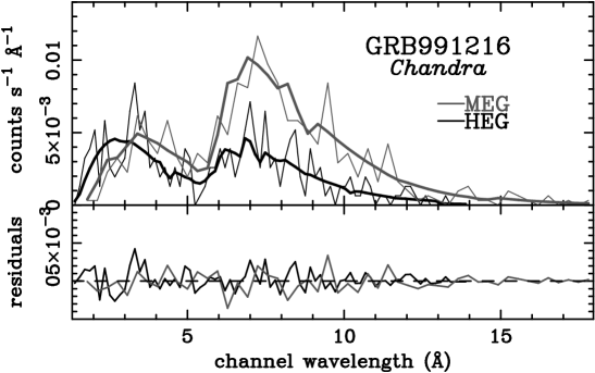
Figure 5: Same as in Figure 1 for the dispersed spectrum of GRB991216.

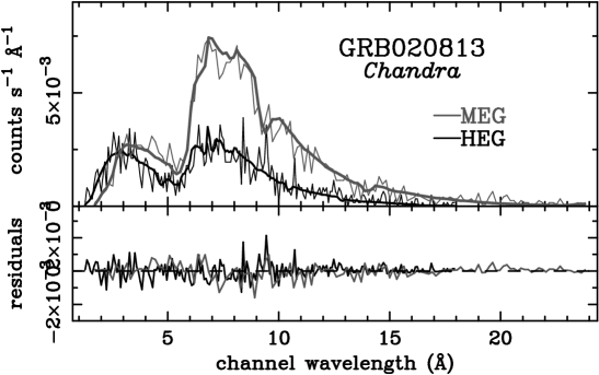
Figure 19: Same as in Figure 1 for the dispersed spectrum of GRB020813.

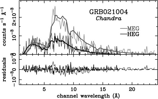
Figure 21: Same as in Figure 1 for the dispersed spectrum of GRB021004.

Figures 1 – 32 show the binned spectra, and $\chi$ value for each spectral bin for the respective best-fit model. Table 3 lists the best-fit parameters and the resulting $\chi^{2}$ and null-hypothesis probability, $P(\chi,\nu)$. We do not list $P(\chi,\nu)$ for the dispersed grating spectra because they were fit with a $C$-statistic due to the low number counts detected per spectral bin. The sample as a whole is consistent with the hypothesis of absorbed power law X-ray emission; out of 27 separate spectra that are fit using $\chi^{2}$-minimization, four have $P(\chi,\nu)<0.1$, consistent with what one would expect statistically from a uniform sample. If we consider the four spectra with $P(\chi,\nu)<0.1$; the zeroth order spectrum of GRB991216, GRB000214, the zeroth order spectrum of GRB021004, and the zeroth order spectrum of GRB030328 (Figures 6, 8, 22, and 27, respectively), only GRB991216 and GRB000214 appear to show discrete residuals suggestive of statistically significant line features. Examination of the other spectra shows one other interesting case, GRB970828 segment B (Figure 4), where the residuals appear to be concentrated in a broad feature (although $P(\chi,\nu)$ is acceptable). As we discuss in the following section, however, the $\chi^{2}$ statistic is not sensitive to weak and/or localized fluctuations, so the $\chi^{2}$ values are not in general particularly useful for line searches. Similarly, $F$-tests yield unreliable values for the significances of line-like features as described in detail by Protassov et al. (2002).

5 Monte Carlo Simulations

As discussed in the previous section, the spectra of most sources are consistent with an absorbed power-law model. However, since the $\chi^{2}$ statistic is not sensitive to small but systematic deviations that would result, for example, from the presence of a weak narrow line, the true null hypothesis probability may be lower than that inferred from the $\chi^{2}$ statistic. In addition, the presence of a weak line may be overlooked when the spectra are binned to contain at least 20 counts per bin so that the $\chi^{2}$ statistic can be used for parameter fitting.

In this section, we describe the Monte Carlo (MC) simulations that are performed to test whether any of the discrete, unresolved line-like features are statistically significant. The method is identical to that adopted by Rutledge & Sako (2003), which was used to estimate the multi-trial statistical significance of the reported soft X-ray features observed in the spectrum of GRB011211 (Reeves et al., 2002). We briefly summarize the procedures below.

For each source spectrum and time interval, we perform $10^{5}$ simulations based on the respective best-fit models. We denote the detected number of photons (source plus background events that lie within the extraction region and time selection) by $C_{\rm{tot}}$ and the estimated number of background photons by $C_{\rm{bkg}}$, where $C_{\rm{tot}}>C_{\rm{bkg}}$. Since we do not know the true number of source photons and hence the source flux, we simulate a fixed number of source plus background photons. The number of background photons is estimated using a Poisson deviate with an average of $C_{\rm{bkg}}$ counts. Background events are randomly selected from analytic background spectral models, which are derived from fits to the spectra obtained from off-axis regions of the same data sets (Chandra and XMM-Newton) or from long blank field observations (ASCA and Beppo-SAX).

We generate counts spectra $I_{j}$ for each simulation and convolve it through a matched filter to compute the $C(E_{i})$ values defined as,

$$C(E_{i})=\sum_{j[E_{i}+3\sigma(E_{i})]}^{j[E_{i}-3\sigma(E_{i})]}I_{j}\frac{1}{\sqrt{2\pi}\sigma(E_{i})}~{}{\rm exp}\left[-\frac{1}{2}\left(\frac{E_{i}-E_{j}}{\sigma(E_{i})}\right)^{2}\right]\delta E_{j},$$ (2)

where $E_{i}$ is the energy in ke V of PI channel $i$ and $\sigma(E_{i})$ is the energy-dependent gaussian width of the instrument response kernel (see, Rutledge & Sako 2003). For each instrument, the shape of the response kernel is extracted at five energies – 0.5, 1, 2, 5, and 10 ke V – from their respective response matrices and fit to a gaussian model. The best-fit $\sigma(E)$ at these five points are then fit to a quadratic function of energy of the form,

$$\sigma(E)=c_{0}+c_{1}E_{\rm{ke~{}V}}+c_{2}E_{\rm{ke~{}V}}^{2},$$ (3)

where $E_{\rm{ke~{}V}}$ is the energy in ke V. The values for $c_{i}$ derived in this manner for each of the instrument are listed in Table 4, and they reproduce the energy dependence of $\sigma$ to within $\sim 20$% across the entire bandpass. The response kernels, in general, are asymmetric and non-gaussian. However, a gaussian reproduces the core of the kernel fairly well, and the results are not sensitive to their exact shapes outside of the core. For the HEG and MEG, we adopt a cubic polynomial of the form,

$$\sigma(\lambda)=c_{0}+c_{1}\lambda_{\mbox{\small\AA}}+c_{2}\lambda_{\mbox{\small\AA}}^{2}+c_{3}\lambda_{\mbox{\small\AA}}^{3},$$ (4)

where the $\lambda_{\mbox{\small\AA}}$ is the wavelength in Å. We adopt the parameters $c_{i}$ as listed on the MIT HETG web site. We list them in Table 4 for completeness. Finally, for the LEG, we assume a constant wavelength dispersion of $\sigma=0.0195$ Å, which is a good approximation in the $2-20$ Å region.

As emphasized by Rutledge & Sako (2003), this procedure maximizes the signal-to-noise of line-like features with intrinsic widths that are smaller than or comparable to the instrument response. For spectra acquired with the CCD, the search is sensitive to lines with widths narrower than $v\sim 10,000~{}\rm{km~{}s}^{-1}$. For the handful of high-resolution spectra in our sample, however, the velocity range spanned by adopting the instrument width is rather limited ($v\sim 1000~{}\rm{km~{}s}^{-1}$). In these cases, we use widths that are up to 16 times the instrument width to search for potentially broader lines as well.

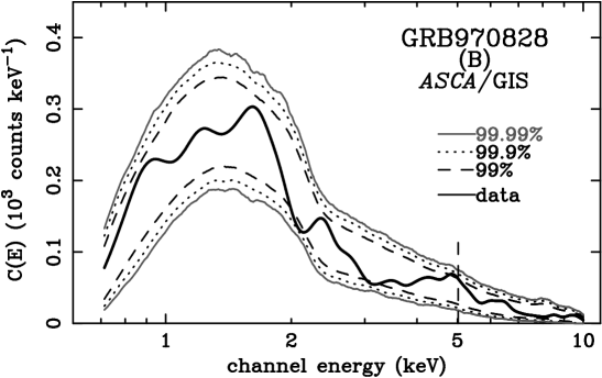
Figure 37: Same as in Figure 33 for GRB970828 GIS time section B.

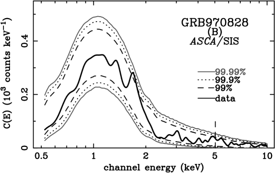
Figure 38: Same as in Figure 33 for GRB970828 SIS time section B.

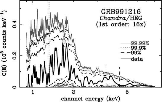
Figure 40: Same as in Figure 33 for GRB991216 first order HEG.

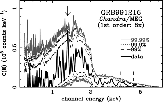
Figure 41: Same as in Figure 33 for GRB991216 first order MEG.

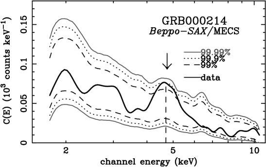
Figure 43: Same as in Figure 33 for GRB000214 MECS.

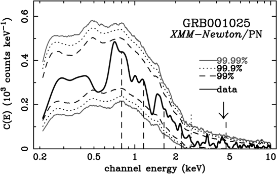
Figure 45: Same as in Figure 33 for GRB001025 PN.

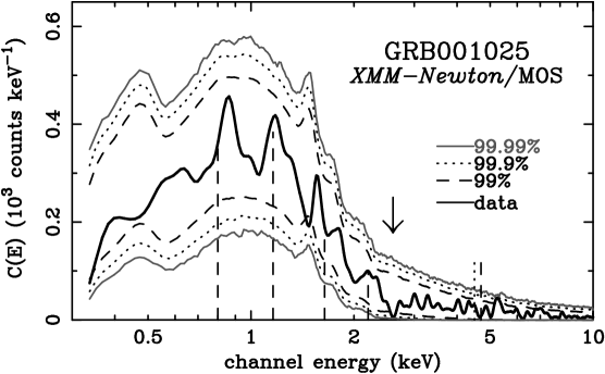
Figure 46: Same as in Figure 33 for GRB001025 MOS.

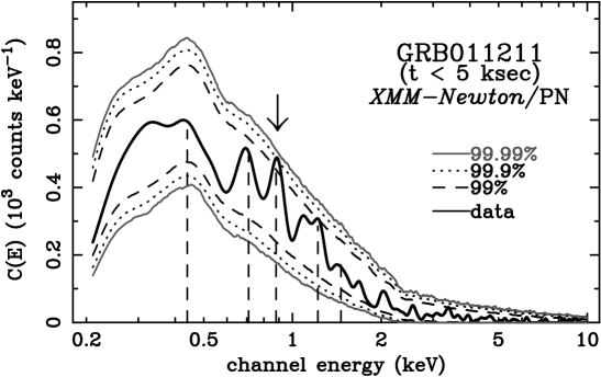
Figure 49: Same as in Figure 33 for GRB011211 PN first 5 ksec.

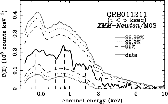
Figure 50: Same as in Figure 33 for GRB011211 MOS first 5 ksec.

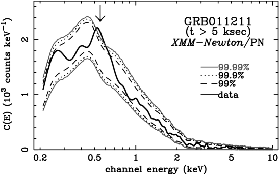
Figure 51: Same as in Figure 33 for GRB011211 PN $t>5$ ksec.

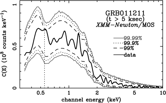
Figure 52: Same as in Figure 33 for GRB011211 MOS $t>5$ ksec.

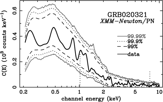
Figure 53: Same as in Figure 33 for GRB020321 PN.

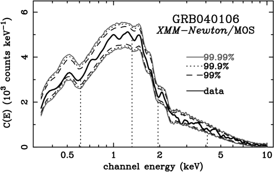
Figure 84: Same as in Figure 33 for GRB040106 MOS.

For each spectral bin, we then sort the $10^{5}$ $C(E_{i})$ values in increasing order and draw the 1000th, 100th, and 10th highest values as the 99%, 99.9%, and 99.99% single-trial significance levels, respectively, as a function of energy. Similarly, we take the 1000th, 100th, and 10th lowest points, which represent 99%, 99.9%, and 99.99% lower limits, to identify possible absorption features in the spectra. The data are convolved in the exact same manner as the simulated events, and we compare the values of each energy bin to the upper and lower bounds. Figures 33 – 84 show the results for each source.

We search through the matched-filtered spectrum for line-like features that exceed or fall below a certain confidence level. If a significant feature is found, the single-trial significance at the peak of the feature is recorded. We then return to the MC simulations and count the ones that contain one or more features that meet or exceed that same single-trial limit at any arbitrary energy. The number of such simulations are recorded and divided by the total number of simulations performed to yield the true multi-trial significance. Qualitatively, the multi-trial probability of detecting a line is higher by a factor of approximately the total number of resolution elements in the detector bandpass. For example, an emission feature with a single-trial significance of $99.99$% (i.e., occurs once in $10^{4}$ random trials at the specified energy) in a detector with $100$ resolution elements is seen approximately once in $\sim 100$ random trials at an arbitrary energy. The energy dependence of the resolving power and the effective area, however, complicates this and the simplest way to address this is through MC simulations.

This method provides a robust estimate of the statistical significances of discrete, unresolved features observed in the spectra, assuming the energy of the feature is not known a priori. Reeves et al. (2003), Watson et al. (2002a) and Watson et al. (2003a) adopt a different method, where each of the simulated spectra are fit by models with and without emission lines. The changes in $\chi^{2}$ are, then, recorded and compared to the observed $\Delta\chi^{2}$ derived from the data. This method should, in principle, yield the probability that the observed features are due to chance coincidences. In practice, however, the significances derived using this method will be overestimated since, as described by Rutledge & Sako (2003), an automated $\chi^{2}$-minimization is almost never capable of finding a true global minimum when the $\chi^{2}$ surface is complicated and contain multiple local minima, for example, when the model involves multiple emission lines. Therefore, the inferred $\Delta\chi^{2}$ between the models with and without emission lines for each simulation is underestimated. This is why the statistical significance derived by Reeves et al. (2003) for the features in the GRB011211 spectrum is significantly higher compared to that of Rutledge & Sako (2003).

Finally, we make explicit our conventions for quoting an ”equivalent gaussian sigma” for a given significance. When the MC simulation of $M$ trials produces $N$ values in excess of that observed at any given energy (single-trial), we give the probability of having observed such a high value produced from noise alone as $p_{\rm excess}=N/M$. This probability includes all phase-space for the observable, both above and below the median. Note that if our observed value is exactly at the median, then $p_{\rm excess}=0.5$.

We then quote a ”equivalent gaussian sigma” for this probability. This provides a short-hand and intuitive denotation of the significance of the observation. We adopt the convention that, for a probability $p_{\rm excess}$ of producing a value at or above the observed value from noise alone, the equivalent gaussian sigma $n$ is found from

$$p_{\rm excess}=\frac{1}{\sqrt{2\pi}}\int_{n}^{\infty}e^{-x^{2}/2}dx,$$ (5)

which means that, for a measured value at the median of the simulated distribution ($p_{\rm excess}$=0.5), this would be $0\sigma$ in excess of the median value. We would call this feature to be signficant at the $0\sigma$ level – and it would not be regarded as a detection of anything. In the case that $p_{\rm excess}=2\times 10^{-5}$, then $n=-4\sigma$ – or, a 4$\sigma$ deficit in counts beneath the median, which would be a significant detection of an absorption line-like feature.

When multi-trial signficances as estimated by counting the $N^{\prime}$ simulations that show emission features with single-trial significances above a certain value, the equivalent gaussian sigma $n^{\prime}$ is derived from

$$p_{\rm excess}=\sqrt{\frac{2}{\pi}}\int_{n^{\prime}}^{\infty}e^{-x^{2}/2}dx.$$ (6)

which is a a one-sided distribution – i.e., if all of the MC simulations show an excess, then the significance is $0\sigma$. In comparison with Equ. 5, Equ. 6 gives a slightly higher value for the equilvalent gaussian sigma for the same $p_{\rm excess}$. Antonelli et al. (2000), Watson et al. (2002a), Butler et al. (2003b), and Watson et al. (2003a) have adopted Equ. 6 in deriving the equivalent gaussian sigma. The differences are relatively small especially at higher significances.

6 Results of the Line Searches

As shown in Figures 33 – 84, there are a number of discrete line-like features that exceed the $99.9$% limit, which approximately corresponds to $3.1\sigma$ at that particular energy (single trial) assuming a gaussian distribution of counts. In 26 cases listed in Table 5, the single-trial confidence exceeds $99.9$% ($3.1\sigma$).

As we have noted earlier, we do not know a priori the expected energies of the lines, even in cases where the source redshift is known, since in some models the line emitting material can have an arbitrary velocity. In such cases, the relevant quantity is the chance probability of detecting any feature that exceeds the $99.9$% limit ($3.3\sigma$, multiple trials). As shown in the final column of Table 5, we find signals which meet this confidence limit in four datasets: in GRB011211 (at time $t>$5 ksec), GRB030227 (the complete dataset), GRB021004, and in GRB040106.

Below, we first discuss our results in comparison with previous reports of line detection, followed by discussion of the four datasets with features with multi-trial probabilities with $>3.3\sigma$ gaussian equivalent significance.

6.1 Comparison with Previous Reports of Line Detection

Below we compare our results to cases where line detections have been claimed in the published literature.

GRB970508: Piro et al. (1999a) reported an unresolved line feature at 3.5 ke V with a significance of $99.3$% ($2.7$$\sigma$) during time interval 1a during part of the afterglow. We find no evidence for a significant excess at 3.5 ke V, or any energy (see Figure 33) during the same time interval. The single-trial confidence at 3.5 ke V is $\sim 60$% ($\sim 0.25\sigma$). The corresponding multi-trial confidence limit is only $\sim 15$% ($\sim 0.2$$\sigma$).

GRB970828: We find no evidence of any single-energy feature similar to the one claimed by Yoshida et al. (1999) during time interval B. However, the reported feature was claimed to be resolved with a centroid of $E=5.04^{+0.23}_{-0.31}~{}\rm{ke~{}V}$ and a width of $\sigma=0.31^{+0.38}_{-0.31}~{}\rm{ke~{}V}$ (Yoshida et al., 1999, 2001). We see an excess at a similar energy in the both the SIS and GIS data (Figure 38 and 37), with single-trial significances of 99.2% (2.4$\sigma$) and 99.4% (2.5$\sigma$), respectively. Our estimate of the multi-trial significance is only $\sim 70$% ($\sim 1.0$$\sigma$) in each instrument. Searches for lines with larger widths resulted in those with lower significance. It is interesting, however, that the residuals of the power-law model fit visually show excesses in all four detectors (see Figure 4). We also note that the S/N in this spectral range is only of order unity, which implies that the estimated significance is highly-dependent on the exact shape and magnitude of the local background spectrum. The reality of this excess feature should, therefore, be taken with caution.

GRB991216: In the case of the GRB991216 Chandra spectrum, where a 4.7$\sigma$ detection of an emission line at $E\sim 3.5~{}\rm{ke~{}V}$ has been claimed (Piro et al., 2000), we instead find only a $99.0$% ($\sim 2.3\sigma$) confidence single-trial fluctuation in the dispersed HEG spectrum at a width of 16 times it’s instrument resolution or FWHM $\sim 0.7$ ke V (see Figure 40), which is close to value quoted in Piro et al. (2000). This fluctuation is at a slightly higher energy ($\sim 3.8$ ke V). Our multi-trial confidence limit of this feature is 20% ($0.3$$\sigma$). We do not find any feature near $4.4\pm 0.5$ ke V, as reported as a marginal detection by Piro et al. (2000). The zeroth order spectrum appears to show an excess feature centered at $E\sim 3.4$ ke V, which is below that seen in the dispersed spectrum, (see 39), but is not significant. Searches for significant features that are narrower than 16 times the HEG resolution resulted in a non-detection.

At least part of the source for the discrepancy between the results of our analysis and that of Piro et al. (2000) is the adopted continuum level. Piro et al. (2000) use a power-law slope and flux determined from the zeroth order spectrum. However, as can be seen in their Figure 1, this continuum systematically underestimates the flux across the entire HETG bandpass. Any fluctuation is, therefore, in excess of the adopted continuum flux. If we allow for a $\sim 20$% calibration uncertainty between the zeroth and first orders, the spectra of both orders are well-represented by a single continuum and, as a consequence, the single-trial significance of the line decreases to $2.3\sigma$ at a single energy. Inspection of the GRB020813 and GRB021004 spectra, both of which were collected in the same instrument configuration, also show a consistent systematic $\sim 20$% discrepancy in the normalizations between the zeroth and first orders.

Incidentally, we note that a feature seen in the MEG at $E\sim 1.32~{}\rm{ke~{}V}$ is of relatively higher significance than the $E\sim 3.5~{}\rm{ke~{}V}$ feature reported by Piro et al. (2000), although it is still extremely marginal. The formal significance is 99.91% single trial ($\sim 3.1$$\sigma$) and 89.2% multi-trial confidence ($\sim 1.6$$\sigma$).

GRB000214: Antonelli et al. (2000) find a feature at $E\sim 4.7~{}\rm{ke~{}V}$ feature which they claim, using an $F$-test to be significant at $99.73$% at a single energy. In our simulations, we find a broad excess at similar energy (Figure 43), significant at $\sim 99.92$% ($\sim 3.2\sigma$) at a single energy. This is slightly higher than found by Antonelli et al. (2000). However, since the redshift is not known, the appropriate multi-trial significance is $99.03$% ($\sim 2.6\sigma$).

GRB001025: Watson et al. (2002a) find a plasma model to be a better fit to the spectrum of this GRB than an absorbed power law, due to a soft excess observed between $\sim 0.5$ and 2 ke V. We find no significant excess at these energies (Figures 10, 45, and 46). The single-trial probabilities are all $<99.9$% confidence, which is below that found with identical instrumentation for GRB011211 (see below). The multi-trial significance of the most significant feature ($\sim 0.7$ ke V excess seen in the PN) is $\sim 65$%.

GRB010220: Watson et al. (2002a) claim the existence of a feature in the PN spectrum of this afterglow at 3.9 ke V. As shown in Figures 11 and 47, we find no evidence for features at any energy being detected with single-energy significance $>$99% confidence (2.3$\sigma$). The multi-trial significance limit would be, consequently, less than that found for GRB001025 (see above), which is $<65$% confidence ($<0.9$$\sigma$).

GRB011211: In GRB011211 the presence of several soft X-ray emission lines from mid-$Z$ elements during the first $5~{}\rm{ksec}$ of the observation has been claimed (Reeves et al., 2003, 2002). We find one feature in the PN spectrum at $E=0.85~{}\rm{ke~{}V}$ with $99.9$% single-trial significance (see Figure 49), coincident with a line Reeves et al. (2002) identified with 97% confidence. This is consistent with the results of Rutledge & Sako (2003) and Borozdin & Trudolyubov (2003). The chance probability of finding such a feature at an arbitrary energy is $\sim 15$% ($1.4\sigma$).

In the spectra acquired during the latter ($t>5$ ksec) time interval, there is an excess feature in the PN spectrum (Figure 51) near the instrumental oxygen edge just above $E\sim 0.5~{}\rm{ke~{}V}$. This feature is statistically significant at the $>99.99$% level at an arbitrary energy, so the formal confidence is $>3.89\sigma$. The feature is not seen in the MOS spectrum, which as an exposure (in cm² s) a factor $\sim 3$ smaller at this energy. We cannot exclude the possibility that the excess is due to calibration uncertainty near the oxygen edge, although no such features have been reported in other high SNR data, nor did we find an excess at this energy in our analysis of the continuum source 3C273 (see below). What makes this particular case somewhat suspicious is that the background spectrum shows an excess similar to the one seen in the GRB spectrum.

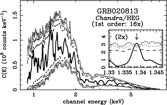
Figure 60: Same as in Figure 33 for GRB020813 HEG dispersed spectrum.

GRB020813: Butler et al. (2003b) have reported evidence for a line at 1.3 ke V. We do find a narrow fluctuation at approximately this energy in the HEG spectrum at $\sim 99.99\%$ confidence (Figure 60), single trial. The multi-trial confidence is, however, only 97.86% (2.3 $\sigma$). Note that the decrease in confidences between single-trial and multi-trial is greater for grating observations, due to the larger number of independent resolution elements in grating spectra.

Inspection of the raw counts in each of the dispersion orders shows an excess in only the $m=+1$ order of the HEG. Of the four spectral orders that are considered ($m=\pm 1$ in HEG and MEG), this is the one with the lowest effective area in this spectral range. The feature is not detected in any of the other spectral orders including the zeroth order. In particular, the effective area of the MEG $m=-1$ order is $\sim 4$ times larger than that of the HEG $m=+1$, which makes the reality of this detection somewhat suspicious.

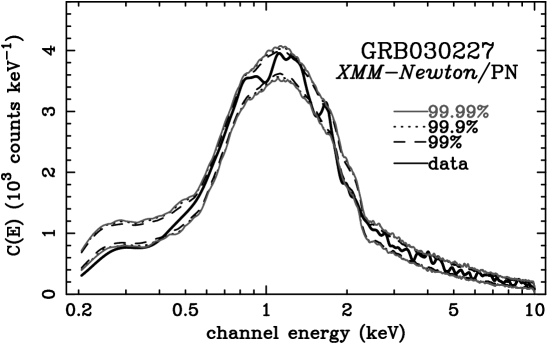
Figure 66: Same as in Figure 33 for GRB030227 PN cumulative spectrum.

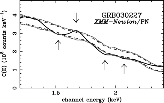
Figure 67: A blow-up of Figure 66 in the 1.2 – 2.4 ke V region.

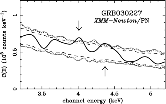
Figure 68: A blow-up of Figure 66 in the 3.2 – 5.2 ke V region.

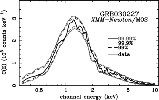
Figure 69: Same as in Figure 33 for GRB030227 MOS cumulative spectrum.

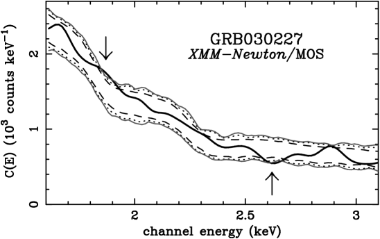
Figure 70: A blow-up of Figure 69 in the 2.1 – 3.1 ke V region.

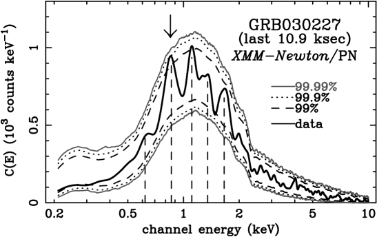
Figure 71: Same as in Figure 33 for GRB030227 PN last 10.9 ksec.

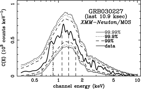
Figure 72: Same as in Figure 33 for GRB30227 MOS last 10.9 ksec.

GRB030227: This is the second highest signal-to-noise observation in our sample only after GRB040106. Watson et al. (2003a) find four emission lines between 0.62 and 1.67 ke V in the last 11 ksec of the PN spectrum of this event. In our analysis (Figures 66 – 72), we find no significant (at $>99.9$%) features in the spectrum during this time interval (a feature near 0.84 ke V is close to 99.9% confidence, single trial). The most significant feature, with single-trial detection confidence of $\lesssim 99.9$%, has multi-trial detection confidence of $<85$% ($<1.4$$\sigma$).

We do, however, find several fluctuations that are in excess of the 99.99% limits in the cumulative PN and MOS spectra (Figures 66 and 69). One of these is in the $1.60-1.69$ ke V range, coincident with a feature identified previously by Mereghetti et al. (2003). However, the multi-trial significance is marginal (98.93% confidence detection; 2.6$\sigma$). Two features at $3.95-4.06$ ke V and $4.33-4.39$ ke V have multi-trial significance greater than 3.3$\sigma$ (3.54$\sigma$ and 3.62$\sigma$, respectively). The former is particularly interesting, since there is a feature at approximately the same energy ($E\sim 3.9~{}\rm{ke~{}V}$) in the MOS as well, just above the 99.9% limit.

The background spectra of the PN or the MOS both do not show discrete features near this energy. To check for other possible calibration uncertainties, we have analyzed the XMM-Newton data of a featureless continuum source, 3C273, to see whether excesses of similar significance do indeed appear in the spectra of other sources. We have extracted only a small fraction of the events so that the spectrum contains the same number of counts in the 1 – 5 ke V range as in the GRB030227 spectrum. We fit the data to an absorbed power-law model and performed MC simulations to derive formal significances of the local fluctuations. Interestingly, no features in excess of 99.99% single-trial confidence were detected in either the PN or the MOS data of 3C273.

In summary, in most cases where lines have been claimed, we either find the fluctuations to be of lower significance, or to be absent. A 3$\sigma$ feature at a given energy in a spectrum with few counts visually appears more significant (i.e., higher equivalent width) than in a spectrum of high statistical quality. These fluctuations are also transient and would appear only during a segment of the total exposure. This trend is similar to the ones seen in many observations in the sense that (1) the “lines” are transient, (2) almost always $\sim 3\sigma$ irrespective of the statistical quality of the data, and (3) high equivalent width.

6.2 Other Sources that Exhibit Line-like Fluctuations

As summarized in Table 5, several sources other than those reported in the literature show features in excess/deficit of the 99.9% single-trial upper/lower limits. Six of these features in four spectra meet a 3$\sigma$ multi-trial significance cut-off:

1. GRB011211: As discussed in §6.1, this source shows a highly significant excess in the $0.51-0.64$ ke V energy range, with a multi-trial significance in excess of 3.89$\sigma$. If modeled as a gaussian line, the feature is unresolved with a centroid of $E=0.58$ ke V. The observed line flux and equivalent width ($EW$) in the PN data is $F=1.1\times 10^{-5}$ photons cm^-2 s^-1 and $EW=70$ eV, respectively. This is one of the two most statistically significant excess in the present analysis. The 1$\sigma$ upper limit in the MOS data is $EW=27$ eV. The rest frame energy for this feature is $E=1.6-2.0$ ke V, which corresponds to a K-shell transition array of neutral to hydrogen-like Si. The excess at this same energy in the background spectrum (discussed above), however, makes this case somewhat suspicious. We leave further analysis with a refined calibration to future work.

2. GRB021004: One feature in the zeroth order spectrum at $E=1.60-1.69$ ke V is significant at $>99.99$% ($>3.72$$\sigma$) single-trial and at $99.92$% ($3.35$$\sigma$) multi-trial. This feature lies below the lower 99.99% limit, which implies an absorption feature. The line is again unresolved, with a centroid of $E=1.64$ ke V. The absorption line flux and equivalent widths are $F=-1.0\times 10^{-6}$ photons cm^-2 s^-1 and $EW=-91$ eV, respectively. The rest frame energy of $E=5.3-5.6$ ke V does not correspond to any strong atomic transition. An obvious feature at the same energy is not observed in the dispersed high resolution spectrum, with a 1$\sigma$ lower limit of $-26$ eV, but is still consistent with the zeroth order spectrum.

3. GRB030227: We find six features in the PN spectrum and two in the MOS spectrum which have single trial confidence levels $>$99.99%; two of these have multi-trial confidences levels $>3\sigma$ observed in the PN detector. The centroids are at $E=4.00$ ke V and $E=4.36$ ke V, with emission line fluxes of $F=1.0\times 10^{-6}$ photons cm^-2 s^-1 and $F=1.1\times 10^{-6}$ photons cm^-2 s^-1, respectively. The corresponding equivalent widths are $EW=66$ eV and $EW=83$ eV. The upper limits derived from the MOS spectra are $EW=93$ eV and $EW=32$ eV for the $4.00$ ke V and $4.36$ ke V features, respectively. The host redshift is not known and so the features cannot be identified with known atomic transitions.

4. GRB040106: Three features in the PN and one in the MOS have single-trial significances in excess of 99.9%. The feature at $\sim 0.6$ ke V is formally significant at $>3.89$ $\sigma$, and its structure is similar to the one detected in the $t>5$ ksec of GRB011211. The corresponding flux observed in the PN detector is $F=1.4\times 10^{-5}$ photons cm^-2 s^-1 ($EW=39$ eV) with a line centroid of $E=0.66$ ke V. The upper limit derived from the MOS data is $F=9.1\times 10^{-6}$ photons cm^-2 s^-1 ($EW=26$ eV). The $\sim 1.33$ ke V feature is an absorption line-like feature with a multi-trial confidence of $99.89$% or 3.26$\sigma$. The absorption flux observed in the PN spectrum is $F=-2.2\times 10^{-6}$ photons cm^-2 s^-1 ($EW=-18$ eV), and the lower limit in the MOS data is $F=9\times 10^{-7}$ photons cm^-2 s^-1 ($EW=7$ eV). Once gain, since no redshift measurement of the host is available to date, we cannot identify any of the features with strong atomic transitions.

6.3 Measurements of Equivalent Hydrogen Column Density in the Host

Galama & Wijers (2001) analyzed eight GRB X-ray afterglows, of which only one of them (GRB970508) is part of our sample, and found that they show evidence for absorption in excess of the Galactic line of sight values. If the absorbing material is at the redshift of the GRB, the columns are large, so that combined with low $A_{V}$ as measured from multi-color optical data, Galama & Wijers (2001) take this to be evidence for dense ionized material surrounding the progenitor. The low $A_{V}$ values can be accounted for by assuming the material is ionized by radiation from the explosion.

If we consider all of our measurements, 14 out of the 21 total have a host column with either a best-fit value of zero, or within 2$\sigma$ of zero (Table 3). In four cases, GRB970508, GRB020322, GRB020405, and GRB030227, there is strong evidence for non-zero host $N_{H}$ at $\geq 4\sigma$, where the error includes only statistical uncertainty, but does not include any estimate of the error in the assumed Galactic $N_{H}$. Of the three most significant (GRB020322, GRB030227, and GRB031203) the host redshift of two (GRB020322 and GRB030227) is, unfortunately, unknown (we assume $z=1$), so the measurement is problematic. GRB031203 does appear to exhibit a column density that is slightly higher, though statistically significant, than that of Dickey & Lockman (1990), but it is consistent with the dust echo measurements as described in Vaughan et al. (2003). Therefore, in a majority of cases, we find no evidence for significant absorbing columns local to the burst. Of course, columns less than a few times 10²¹ cm^-2 are difficult to measure given the significant redshifts for the events.

Stratta et al. (2004) examined 13 afterglows observed with Beppo-SAX, which includes the two sources presented in this paper, and found that 2 sources show highly-significant absorption above the Galactic value. Both GRB970508 and GRB000214 do not appear to show any obvious signatures of substantial host galaxy absorption, which is consistent with what we find. The upper-limits they derive for the remaining 11 sources are comparable to or above the magnitude of the detections, as are the upper-limits we derive, implying that the non-detections are due to instrumental sensitivity.

6.4 Consistency with Prior Detection Claims

Our analysis at first glance appears to be inconsistent with previous work, in that we do not confirm any prior claimed detection to be significant. In addition, the most significant deviations we find have not been previously reported, even in spectra with published analyses. In some cases we find deviations at the reported energy, but at statistical significance substantially lower than claimed. In a few cases we do not see positive fluctuations at the claimed energy, and in three cases we find fluctuations at $>3$$\sigma$ that have not been reported in spectra analyzed by others. An important point to note is that our analyses, by no means, rule out the possibility of discrete features in any of the spectra. The presence of weak features is certainly possible, but, in most cases, they are not required by the data in a model-independent way.

In most cases we can understand the origin of the discrepancy. In GRB991216 we disagree with the continuum level adopted by Piro et al. (2000). If the continuum model lies below most of the data points (see Figure 1 of Piro et al. 2000), the inferred significance of the line would consequently be overestimated, although we find that renormalizing the continuum to the one adopted by Piro et al. (2000) yields a single-trial significance of $\sim 3.2$$\sigma$, which is still lower than claimed by those authors ($\sim 4.7$$\sigma$). In most other cases, we have probably adopted different background regions for subtraction, so that if reported features are background fluctuations, we would expect to find them at different energy, or at different level depending on the exact background region used. In any case, a robust detection should not be highly-sensitive to the exact nature of the assumed background spectrum.

Our analysis results are in rough agreement with most of those published recently by Butler et al. (2004), who have also re-analyzed a small subset of the data presented here using a similar statistical approach. There are, however, notable differences in the quoted multi-trial significances of the features in the high-resolution grating spectra of GRB991216 and GRB020813. They find that the claimed feature in the first order spectrum of GRB991216 (Piro et al., 2000) is significant at $>3.7$$\sigma$ multi-trial, while our analysis yields a significance of at most $\sim 1.3$$\sigma$ (see, also, Figure 40 and 41). Similarly, they find that the significance of the line claimed in GRB020813 by Butler et al. (2003b) is $3.5$$\sigma$ multi-trial, while we find it to be significant at only $2.7$$\sigma$. These discrepancies are most likely due to the fact that Butler et al. (2004) choose to simulate counts based on their spectral fit to unbinned spectra, which predicts a count rate that is lower than the observed value. This means that fluctucation present in the spectrum appear preferentially as positive emission line-like fluctuations. We believe that our approach of fixing the number of simulated counts to the obseved value is more robust, unless there are good reasons to believe a priori that the true continuum level is lower than what one infers from a blind fit.

We point out that a true multi-trial significance should also account for the total number of spectra inspected, and depends on whether the observation was divided into several time segments or if data from more than one detector with comparable S/N and spectral coverage were available. It appears that none of the authors have properly derived the significances of the features that are seen only in selected time segments of a longer observation and in a single detector. For example, if a $3\sigma$ line is detected only in the PN spectrum aqcuired in the first 5 ksec of a 40 ksec exposure, then the true multi-trial probability that this is not due to a statistical fluctuation is $\sim 2\times 40/8=10$ times lower or $\sim 2.2\sigma$ (the factor of $\sim 2$ comes from the fact that the two MOS cameras combined provide data of comparable sensitivity). If the S/N for each time segment and/or detector are not identical, one must carefully weigh each trial by estimating its sensitivity to the detection of the line seen in the other dataset(s).

In all cases, the authors have not explicitly stated all of the time segments used in their line searches. As stated earlier, none of the features are observed in more than one detector and this has not been factored into their derived significances. We have not factored these criteria into the quoted significance for the features that we detect either, since we make no claims as to the reality, interpretation, or ubiquity of features such as the ones that appear in GRB011211, GRB021004, GRB030227, or GRB040106. Rather, we find these to be motivation for significantly higher signal-to-noise observations, and we call into question prior statements regarding the detection of features with a specific interpretation.

7 Summary and Conclusions

We have performed detailed, uniform analyses of 21 of the brightest GRB X-ray afterglows, and have derived the statistical significances of line-like fluctuations that appear in the spectra. We find that in most cases, the data are well-fit by an absorbed power-law spectral model, with the significance of any deviations being marginal. This includes several cases where either lines, or deviations from a power-law continuum have previously been reported at reasonable significance. In particular, this includes GRB970508, GRB970828, GRB991216, and GRB000214 where features from Fe emission have been reported, GRB011211, GRB010220, and GRB030227 where a thermal emission lines from low-$Z$ elements have been claimed, and GRB001025, where one prior analysis found the spectrum to be better described by a thermal emission model than by a power law.

There are four interesting exceptions that we find are worth attention; the cumulative spectrum of GRB030227, the $t>5~{}\rm{ksec}$ spectrum of GRB011211, the zeroth order spectrum of GRB021004, and GRB040106. In addition, there is one interesting case (GRB970828), where a broad excess is visible in all four detectors on ASCA, although the formal significance is marginal and depends highly on the assumed background spectrum.

The absorption line-like feature seen in the zeroth order spectrum of GRB021004 is formally significant at $3.35$$\sigma$ multi-trial. This feature corresponds to an energy of $\sim 5.5$ ke V in the rest frame of the GRB, and does not have an obvious identification. It is not observed in the dispersed spectrum. We also note that there is a local minimum in the effective area at this energy, which makes the feature appear more significant visually, as in the case for GRB991216, where the claimed emission line lies at a local maximum of the efficiency curve.

The $t>5~{}\rm{ksec}$ interval of the GRB011211 spectrum and the cumulative spectrum of GRB040106 both exhibit features at $E\sim 0.5~{}\rm{ke~{}V}$. These are by far the most statistically significant in our sample with multi-trial significances exceeding $3.89$$\sigma$. The host’s known redshift of GRB011211 places the feature at a rest frame of $E\sim 1.7$ ke V, which may be identified as Si K fluorescence, but could easily be due to other elements moving at arbitrary velocities. As noted above, the observed energies correspond also to a local fluctuation in the background spectrum as well as an instrumental absorption edge of atomic or molecular oxygen.

In GRB030227, Watson et al. (2003a) report the detection of multiple emission lines during the last $\sim 11~{}\rm{ksec}$ of the observation. We do not confirm this result and we find that the strongest feature at $E\sim 0.85$ ke V is significant at $\lesssim 99.9$% for a single trial. However, the cumulative spectrum of the entire observation does appear to show fluctuations with substantially higher significance than those reported by Watson et al. (2003a). One of these, at $E\sim 4$ ke V, is significant at 3.54$\sigma$. Unfortunately there is no measured redshift for this event, so the rest-frame energy is unknown.

Although our analysis rules out all of the reported features, we do find some evidence, in four cases, for marginally significant spectral features at energies that do not suggest a clear interpretation. We cannot rule out the possibility that relatively weak line features are present in the X-ray spectra of some, if no all, GRBs. Given the diagnostic power of such detections, longer exposures of bright events are certainly warranted. Our work does, however, call into question the reality of all of the features detected to-date, as well as the interpretation of these features as either iron, or specific low-$Z$ elements.

Swift, which will observe a large number of GRBs early on, when they are bright, has the potential and opportunity to confirm the existence of X-ray line emission. Although the effective area of the Swift X-ray Telescope (XRT) is a factor of $\sim 10$ lower than that of the XMM-Newton PN camera and a factor of $\sim 20$ lower than the combined EPIC effective area, it is capable of collecting data starting only minutes after the burst compared to $\sim 0.5$ days for both XMM-Newton and Chandra. For a flux decay time slope of $\alpha=1-2$, where the X-ray flux $F_{X}\propto t^{-\alpha}$, a typical burst will be $2-3$ orders of magnitude brighter during the beginning of a Swift observation and the XRT data on average will be of higher statistical quality by roughly an order of magnitude. The late afterglow $\gtrsim 0.5$ days after the burst will still be better studied with the CCDs on XMM-Newton, Chandra, as well as ASTRO-E2. If, however, the lines are narrow ($v\lesssim 1000~{}\rm{km~{}s}^{-1}$), the Chandra gratings, the XMM-Newton RGS, and the X-ray Spectrometer on ASTRO-E2 will provide more sensitive measurements on most bursts. Clearly, in any case, this is not a straightforward measurement, and a carefully planned observation strategy is required to maximize the detection probability. Monitoring of the early X-ray flux with Swift and follow-up observations of the brightest afterglows with XMM-Newton, Chandra, and ASTRO-E2 will minimize the risk of obtaining an underexposed spectrum, although this does not by any means guarantee the detection of lines. Of course, the ultimate goal is to take one step further and actually use X-ray spectroscopic diagnostics to infer important physical information about the burst. Note, however, that the physical conditions of the X-ray emission regions during the early afterglow (accessible only with Swift) can be vastly different from those approximately a day after the burst, and it is not clear whether a direct comparison of measurements will be meaningful.

We finally point out that spectral identifications is also not a straightforward task. This is obvious when only a single significant feature is detected, but is also true even when multiple lines are detected in the spectrum. The energies of the hydrogen-like Ly$\alpha$ lines of neighboring abundant metals, for example, are spaced roughly equally and they can be misinterpreted or their identifications can at best be ambiguous. If a significant amount of iron is present, the spectrum may exhibit broad bumps that may dominate over narrow isolated lines from other elements and may not appear as prominent line emission. Although arbitrary bulk velocities can be invoked to match transitions of specific elements, any constraint on the burst redshift (e.g., from optical absorption/emission line measurements) is extremely valuable.

If the combination of Swift, XMM-Newton, Chandra, and ASTRO-E2 is unable to find similar features in spectra with large numbers of counts, then the $\sim 3$$\sigma$ detections found here are likely spurious. If this is the case, tight upper limits on the line fluxes and equivalent widths will provide invaluable constraints on the geometry and chemical abundances of the burst environment, which can then be used as quantitative tests of GRB afterglow models.

Table 1: Observations of Bright GRB X-ray Afterglows

Burst	Mission	Instrument(s)	$T_{\rm{start}}$	Exposure	$z$
970508	Beppo-SAX	LECS & MECS	0.4340	15.4	0.835
970828	ASCA	SIS & GIS	1.1906	33.8	0.9578
991216	Chandra	HETG/ACIS-S	1.5215	9.65	1.02
000210	Chandra	ACIS-S	0.7778	8.93	0.8463
000214	Beppo-SAX	LECS & MECS	0.5237	43.5	$\cdots$
000926	Chandra	ACIS-S	2.6861	10.2	2.066
001025	XMM-Newton	EPIC-PN	1.9092	23.7	$\cdots$
$\cdots$	$\cdots$	EPIC-MOS	1.8814	37.1	$\cdots$
010220	XMM-Newton	EPIC-PN	0.6247	12.1	$\cdots$
011030	Chandra	ACIS-S	10.4592	46.6	$\cdots$
011211	XMM-Newton	EPIC-PN	0.5029	26.8	2.140
$\cdots$	$\cdots$	EPIC-MOS	0.4851	31.2	$\cdots$
020321	XMM-Newton	EPIC-PN	0.4289	36.3	$\cdots$
$\cdots$	$\cdots$	EPIC-MOS	0.4119	40.0	$\cdots$
020322	XMM-Newton	EPIC-PN	0.6428	23.8	$\cdots$
$\cdots$	$\cdots$	EPIC-MOS	0.6222	28.2	$\cdots$
020405	Chandra	LETG/ACIS-S	1.6825	50.6	0.690
020813	Chandra	HETG/ACIS-S	0.7367	76.9	1.254
021004	Chandra	HETG/ACIS-S	0.8533	86.7	2.323
030226	Chandra	ACIS-S	1.5436	36.4	1.986
030227	XMM-Newton	EPIC-PN	0.3604	33.3	$\cdots$
$\cdots$	$\cdots$	EPIC-MOS	0.3440	35.9	$\cdots$
030328	Chandra	LETG/ACIS-S	0.6387	92.7	1.520
030329	XMM-Newton	EPIC-PN	37.0577	29.6	0.1685
$\cdots$	$\cdots$	EPIC-MOS	37.0423	32.4	$\cdots$
$\cdots$	$\cdots$	EPIC-PN	60.3962	38.8	$\cdots$
$\cdots$	$\cdots$	EPIC-MOS	60.3807	46.5	$\cdots$
031203	XMM-Newton	EPIC-PN	0.2723	50.7	0.105
$\cdots$	$\cdots$	EPIC-MOS	0.2567	57.4	$\cdots$
$\cdots$	$\cdots$	EPIC-PN	2.8549	36.5	$\cdots$
$\cdots$	$\cdots$	EPIC-MOS	2.8414	34.4	$\cdots$
040106	XMM-Newton	EPIC-PN	0.2552	37.1	$\cdots$
$\cdots$	$\cdots$	EPIC-MOS	0.2344	42.6	$\cdots$

Table 2: Summary of Reported Emission Lines in the Literature

Burst	Epoch/order	Line Energy (keV)	Line Width (keV)	Model/Identification	Significance ($\sigma$)	Reference
970508	1a	3.5	$\lesssim 0.5$	Fe K$\alpha$	99.3% (2.7$\sigma$)	Piro et al. (1999a)
970828	B	5.03${}^{+0.23}_{-0.31}$	$0.31^{+0.38}_{-0.31}$	Fe XXVI Ly$\alpha$ or RRC	98.3% (2.4$\sigma$)	Yoshida et al. (1999, 2001)
991216	$|m|=1$	$3.49\pm 0.06$	$0.23\pm 0.07$	Fe XXVI Ly$\alpha$	99.99974% (4.7$\sigma$)	Piro et al. (2000)
$\cdots$	$m=0$	$4.4\pm 0.5$	$\cdots$	Fe XXVI RRC	99.5% (2.8$\sigma$)	Piro et al. (2000)
000214	$\cdots$	$4.7\pm 0.2$	unresolved	Fe K$\alpha$	99.85% (3.2$\sigma$)	Antonelli et al. (2000)
001025	$\cdots$	$0.80^{+0.04}_{-0.05}$	$0.10\pm 0.03$	Mg XII	99.94% (3.4$\sigma$)	Watson et al. (2002a)
$\cdots$	$\cdots$	$1.16\pm 0.05$	$\cdots$	Si XIV	99.92% (3.4$\sigma$)	$\cdots$
$\cdots$	$\cdots$	$1.64\pm 0.07$	$\cdots$	S XVI	99.92% (3.4$\sigma$)	$\cdots$
$\cdots$	$\cdots$	$2.2\pm 0.1$	$\cdots$	Ar XVIII	98% (2.3$\sigma$)	$\cdots$
$\cdots$	$\cdots$	4.7${}^{+0.8}_{-0.4}$	$\cdots$	Ni XXVIII	88% (1.6$\sigma$)	$\cdots$
010220	$\cdots$	$\sim 3.9$	unresolved	Ni XXVIII Ly$\alpha$	99.0% (2.6$\sigma$)	Watson et al. (2002a)
011211	($t<5$ ksec)	$0.44\pm 0.04$	unresolved	Mg XI	99.97% (3.6$\sigma$)	Reeves et al. (2003)
$\cdots$	$\cdots$	$0.71\pm 0.02$	$\cdots$	Si XIV	$\cdots$	$\cdots$
$\cdots$	$\cdots$	$0.88\pm 0.02$	$\cdots$	S XVI	$\cdots$	$\cdots$
$\cdots$	$\cdots$	$1.22\pm 0.03$	$\cdots$	Ar XVIII	$\cdots$	$\cdots$
$\cdots$	$\cdots$	$1.46\pm 0.07$	$\cdots$	Ca XX	$\cdots$	$\cdots$
020813	$|m|=1$	$1.31\pm 0.01$	$0.008\pm 0.004$	S XVI Ly$\alpha$	99.90% (3.3$\sigma$)	Butler et al. (2003b)
030227	(last 11 ksec)	0.62${}^{+0.03}_{-0.02}$	unresolved	Mg XII	97% (2.2$\sigma$)	Watson et al. (2003a)
$\cdots$	$\cdots$	0.86${}^{+0.02}_{-0.03}$	$\cdots$	Si XIV	99.98% (3.8$\sigma$)	$\cdots$
$\cdots$	$\cdots$	$1.11\pm 0.02$	$\cdots$	S XVI	99.96% (3.5$\sigma$)	$\cdots$
$\cdots$	$\cdots$	1.35${}^{+0.04}_{-0.03}$	$\cdots$	Ar XVII or XVIII	92% (1.7$\sigma$)	$\cdots$
$\cdots$	$\cdots$	$1.66\pm 0.04$	$\cdots$	Ca XIX or XX	99% (2.5$\sigma$)	$\cdots$
$\cdots$	$\cdots$	1.67${}^{+0.01}_{-0.03}$	$\cdots$	Fe K$\alpha$	99.86% (3.2$\sigma$)	Mereghetti et al. (2003)

Table 3: Continuum Spectral Parameters

Burst	Epoch/order	$C_{\rm{tot}}$	$C_{\rm{bkg}}$	$N_{\rm{H}}^{\rm{Gal}}$	$N_{\rm{H}}^{\rm{host}}$	$\Gamma$	$F_{\rm{1keV}}$	$\chi^{2}/\nu$	$P(\chi,\nu)$
970508	1a	137	34	0.051	$10^{+6}_{-4}$	$3.1^{+0.5}_{-0.4}$	$2.6^{+0.5}_{-0.4}\times 10^{-3}$	2.6/5	0.76
$\cdots$	1b	188	56	0.051	$7^{+11}_{-7}$	$2.0^{+1.0}_{-0.9}$	$3.5^{+0.4}_{-0.3}\times 10^{-4}$	2.4/6	0.88
970828	A+C	1922	953	0.036	$1.5^{+1.2}_{-1.0}$	$2.4^{+0.4}_{-0.3}$	$2.0^{+1.0}_{-0.6}\times 10^{-4}$	100/86	0.14
$\cdots$	B	1215	515	0.036	$0.0^{+0.8}_{-0.0}$	$2.1^{+0.3}_{-0.3}$	$1.7^{+0.6}_{-0.6}\times 10^{-4}$	58/54	0.33
991216	$|m|=1$	762	13	0.20	$0.8^{+0.4}_{-0.3}$	$1.6^{+0.1}_{-0.1}$	$8.2^{+0.5}_{-0.5}\times 10^{-4}$	153/130	$\cdots$
$\cdots$	$m=0$	604	4	0.20	$0.0^{+0.3}_{-0.0}$	$1.7^{+0.1}_{-0.1}$	$6.7^{+0.5}_{-0.5}\times 10^{-4}$	46/32	0.05
000210	$\cdots$	552	2	0.025	$3.7^{+1.1}_{-1.1}$	$1.9^{+0.1}_{-0.1}$	$8.8^{+0.6}_{-0.7}\times 10^{-5}$	26/21	0.22
000214	$\cdots$	378	134	0.058	$0.0^{+1.2}_{-0.0}$	$2.0^{+0.3}_{-0.3}$	$1.4^{+0.5}_{-0.4}\times 10^{-4}$	28/18	0.07
000926	$\cdots$	267	1	0.027	$0.0^{+0.4}_{-0.0}$	$1.9^{+0.3}_{-0.2}$	$3.2^{+0.4}_{-0.4}\times 10^{-5}$	15/13	0.20
001025	$\cdots$	1249	313	0.061	$0.19^{+0.07}_{-0.06}$	$2.6^{+0.4}_{-0.2}$	$2.5^{+0.7}_{-0.5}\times 10^{-5}$	43/63	0.98
010220	$\cdots$	247	124	0.86	$0.1^{+1.3}_{-0.1}$	$1.8^{+1.0}_{-0.4}$	$1.9^{+0.7}_{-0.6}\times 10^{-5}$	6.5/9	0.69
011030	$\cdots$	376	6	0.10	$0.0^{+0.1}_{-0.0}$	$1.5^{+0.3}_{-0.2}$	$1.1^{+0.3}_{-0.1}\times 10^{-5}$	3.1/14	1.00
011211	$t<5$ ksec	936	58	0.042	$0.1^{+0.4}_{-0.1}$	$2.2^{+0.2}_{-0.2}$	$7.8^{+1.0}_{-0.7}\times 10^{-5}$	38/40	0.56
$\cdots$	$t>5$ ksec	3046	294	0.042	$0.2^{+0.2}_{-0.2}$	$2.3^{+0.1}_{-0.2}$	$4.6^{+0.5}_{-0.1}\times 10^{-5}$	99/129	0.98
020321	$\cdots$	1664	487	0.082	$0.02^{+0.06}_{-0.02}$	$2.1^{+0.2}_{-0.3}$	$9.9^{+2.3}_{-2.0}\times 10^{-6}$	33/45	0.91
020322	$\cdots$	5791	1252	0.046	$0.20^{+0.03}_{-0.03}$	$2.3^{+0.1}_{-0.1}$	$1.1^{+0.1}_{-0.1}\times 10^{-4}$	228/241	0.72
020405	$|m|=1$	1242	84	0.043	$0.4^{+0.1}_{-0.1}$	$1.7^{+0.1}_{-0.1}$	$2.6^{+0.1}_{-0.1}\times 10^{-4}$	1364/1318	$\cdots$
$\cdots$	$m=0$	604	4	0.043	$0.6^{+0.3}_{-0.1}$	$2.0^{+0.2}_{-0.1}$	$3.7^{+0.8}_{-0.7}\times 10^{-4}$	32/33	0.49
020813	$|m|=1$	4659	117	0.075	$0.0^{+0.1}_{-0.01}$	$1.8^{+0.1}_{-0.1}$	$6.3^{+0.2}_{-0.2}\times 10^{-4}$	455/348	$\cdots$
$\cdots$	$m=0$	3679	77	0.075	$0.0^{+0.1}_{-0.0}$	$1.8^{+0.1}_{-0.1}$	$5.2^{+0.2}_{-0.2}\times 10^{-4}$	145/142	0.42
021004	$|m|=1$	1634	109	0.011	$0.0^{+0.1}_{-0.0}$	$2.1^{+0.1}_{-0.1}$	$2.0^{+0.1}_{-0.1}\times 10^{-4}$	440/348	$\cdots$
$\cdots$	$m=0$	1252	5	0.011	$0.0^{+0.3}_{-0.0}$	$2.0^{+0.1}_{-0.1}$	$1.6^{+0.1}_{-0.1}\times 10^{-4}$	77/52	0.02
030226	$\cdots$	345	1	0.016	$0.0^{+0.5}_{-0.0}$	$2.1^{+0.2}_{-0.2}$	$1.3^{+0.1}_{-0.1}\times 10^{-5}$	11/13	0.59
030227	total	13676	2348	0.22	$0.60^{+0.04}_{-0.04}$	$1.97^{+0.02}_{-0.02}$	$2.34^{+0.04}_{-0.04}\times 10^{-4}$	303/278	0.12
$\cdots$	last 11 ksec	2777	171	0.22	$0.7^{+0.2}_{-0.2}$	$1.9^{+0.1}_{-0.1}$	$1.8^{+0.2}_{-0.2}\times 10^{-4}$	115/124	0.70
030328	$|m|=1$	562	131	0.043	$0.0^{+0.2}_{-0.0}$	$1.9^{+0.1}_{-0.1}$	$6.6^{+0.5}_{-0.5}\times 10^{-5}$	1172/1318	$\cdots$
$\cdots$	$m=0$	529	18	0.043	$0.18^{+0.17}_{-0.15}$	$2.1^{+0.2}_{-0.1}$	$7.6^{+1.2}_{-1.2}\times 10^{-5}$	30/21	0.09
030329	I	665	80	0.021	$0.00^{+0.03}_{-0.00}$	$2.0^{+0.2}_{-0.2}$	$7.4^{+0.8}_{-0.9}\times 10^{-6}$	37/37	0.48
$\cdots$	II	543	143	0.021	$0.02^{+0.07}_{-0.02}$	$2.0^{+0.3}_{-0.2}$	$3.9^{+0.9}_{-1.1}\times 10^{-6}$	34/31	0.32
031203	I	7012	647	0.59	$0.29^{+0.04}_{-0.03}$	$1.8^{+0.1}_{-0.1}$	$1.1^{+0.1}_{-0.1}\times 10^{-4}$	218/208	0.32
$\cdots$	II	1194	381	0.59	$0.80^{+0.17}_{-0.16}$	$1.9^{+0.1}_{-0.1}$	$5.8^{+0.4}_{-0.4}\times 10^{-5}$	41/50	0.81
040106	$\cdots$	23190	1420	0.086	$0.00^{+0.02}_{-0.00}$	$1.50^{+0.02}_{-0.01}$	$1.88^{+0.05}_{-0.05}\times 10^{-4}$	622/603	0.29

Table 4: Parameters for the Matched Filter Kernel

Instrument	$c_{0}$	$c_{1}$	$c_{2}$	$c_{3}$
SIS	$4.43\times 10^{-2}$	$1.28\times 10^{-2}$	$2.52\times 10^{-5}$	$\cdots$
GIS	$4.13\times 10^{-2}$	$3.82\times 10^{-2}$	$-1.60\times 10^{-3}$	$\cdots$
MECS	$5.20\times 10^{-2}$	$3.32\times 10^{-2}$	$-1.12\times 10^{-3}$	$\cdots$
ACIS	$3.96\times 10^{-2}$	$5.28\times 10^{-3}$	$-1.31\times 10^{-4}$	$\cdots$
MOS	$2.50\times 10^{-2}$	$8.77\times 10^{-3}$	$-2.79\times 10^{-4}$	$\cdots$
PN	$3.42\times 10^{-2}$	$6.63\times 10^{-3}$	$-1.46\times 10^{-4}$	$\cdots$
HEG	$1.00\times 10^{-2}$	$-1.41\times 10^{-4}$	$1.46\times 10^{-5}$	$-1.963\times 10^{-7}$
MEG	$1.89\times 10^{-2}$	$-3.39\times 10^{-4}$	$2.98\times 10^{-5}$	$-4.110\times 10^{-7}$
LEG	$1.95\times 10^{-2}$	$\cdots$	$\cdots$	$\cdots$

Table 5: Summary of Single- and Multi-trial Significances of Features with Single-Trial Significances $>$99.9%

Burst	Instrument	Epoch/order	Energy Range (keV)	Single-trial	Multi-trial
991216	MEG	$|m|=1$	1.317 – 1.326	$99.98$%	$89.20$%
000214	MECS	$\cdots$	4.60 – 4.80	$99.92$%	$99.03$%
001025	MOS	$\cdots$	2.60 – 2.63	$>99.99$%	$99.23$%
011211	PN	$t<5$ ksec	0.88 – 0.91	$99.96$%	$89.09$%
$\cdots$	PN	$t>5$ ksec	0.51 – 0.64	$>99.99$%	$>99.99$%
020321	MOS	$\cdots$	1.01 – 1.03	$99.95$%	$94.85$%
$\cdots$	MOS	$\cdots$	7.58 – 7.66	$>99.99$%	$99.36$%
020322	PN	$\cdots$	6.15 – 6.18	$99.93$%	$89.15$%
$\cdots$	MOS	$\cdots$	2.09 – 2.12	$99.92$%	$80.13$%
$\cdots$	MOS	$\cdots$	4.97 – 5.08	$99.90$%	$72.26$%
020405	LETG	$|m|=1$	0.733 – 0.740	$99.97$%	$98.23$%
$\cdots$	LETG	$|m|=1$	0.941 – 0.953	$99.96$%	$96.98$%
020813	HEG	$|m|=1$	1.303 – 1.322	$>99.99$%	$99.40$%
021004	ACIS-S	$|m|=0$	1.60 – 1.69	$>99.99$%	$99.92$%
030227	PN	total	1.51 – 1.55	$>99.99$%	$98.92$%
$\cdots$	PN	total	1.66 – 1.69	$>99.99$%	$98.93$%
$\cdots$	PN	total	1.80 – 1.96	$>99.99$%	$98.99$%
$\cdots$	PN	total	2.03 – 2.11	$>99.99$%	$98.93$%
$\cdots$	PN	total	3.95 – 4.06	$>99.99$%	$99.96$%
$\cdots$	PN	total	4.33 – 4.39	$>99.99$%	$99.97$%
$\cdots$	MOS	total	1.85 – 1.88	$>99.99$%	$99.25$%
$\cdots$	MOS	total	2.62 – 2.66	$>99.99$%	$99.50$%
040106	PN	$\cdots$	0.54 – 0.70	$>99.99$%	$>99.99$%
$\cdots$	PN	$\cdots$	1.30 – 1.37	$>99.99$%	$99.89$%
$\cdots$	PN	$\cdots$	1.95 – 1.96	$>99.99$%	$98.58$%
$\cdots$	PN	$\cdots$	4.07 – 4.11	$99.94$%	$93.49$%

Figure 1: The observed X-ray spectrum of GRB970508 time segment 1a. In this figure and the similar ones that follow, the top panel shows the data with the best-fit model superimposed. The lower panel shows the resulting $\chi$ for each of the spectral channels, except in the high-resolution Chandra grating data where we plot the flux residuals.

Figure 2: Same as in Figure 1 for time segment 1b.

Figure 3: Same as in Figure 1 for GRB970828 time segments A and C.

Figure 4: Same as in Figure 1 for GRB970508 time segment B.

Figure 6: Same as in Figure 1 for the zeroth order spectrum of GRB991216.

Figure 7: Same as in Figure 1 for GRB000210.

Figure 8: Same as in Figure 1 for GRB000214.

Figure 9: Same as in Figure 1 for GRB000926.

Figure 10: Same as in Figure 1 for GRB001025.

Figure 11: Same as in Figure 1 for GRB010220.

Figure 12: Same as in Figure 1 for XRF011030.

Figure 13: Same as in Figure 1 for GRB011211 time segment 1.

Figure 14: Same as in Figure 1 for GRB011211 time segment 2.

Figure 15: Same as in Figure 1 for GRB020321.

Figure 16: Same as in Figure 1 for GRB020322.

Figure 17: Same as in Figure 1 for the dispersed spectrum of GRB020405.

Figure 18: Same as in Figure 1 for the zeroth order spectrum of GRB020405.

Figure 20: Same as in Figure 1 for the zeroth order spectrum of GRB020813.

Figure 22: Same as in Figure 1 for the zeroth order spectrum of GRB021004.

Figure 23: Same as in Figure 1 for GRB030226.

Figure 24: Same as in Figure 1 for the dispersed spectrum of GRB030227.

Figure 25: Same as in Figure 1 for the zeroth order spectrum of GRB030227.

Figure 26: Same as in Figure 1 for the dispersed spectrum of GRB030328.

Figure 27: Same as in Figure 1 for the zeroth order spectrum of GRB030328.

Figure 28: Same as in Figure 1 for GRB030329 epoch 1.

Figure 29: Same as in Figure 1 for GRB030329 epoch 2.

Figure 30: Same as in Figure 1 for GRB031203 epoch 1.

Figure 31: Same as in Figure 1 for GRB031203 epoch 2.

Figure 32: Same as in Figure 1 for GRB040106.

Figure 33: Upper and lower limits for $C(E)$ derived from Monte Carlo simulations based on the best-fit continuum model parameters for GRB970508 time section 1a. The following figures show the same for the bursts listed in Table 3. The data are represented as thick solid curves, while single-trial 99%, 99.9%, and 99.99% limits as functions of the energy are shown as dashed, dotted, and thin gray solid curves, respectively. Features in excess of the 99.9% limits in our analyses are marked with arrows. Previously claimed detections by other authors are labeled by vertical dashed lines. Finally, the vertical dotted lines represent the energies where a feature is detected at $>99.9$% single-trial confidence in other available instruments or spectral orders.

Figure 34: Same as in Figure 33 for GRB970508 section 1b.

Figure 35: Same as in Figure 33 for GRB970828 GIS time section A and C.

Figure 36: Same as in Figure 33 for GRB970828 SIS time section A and C.

Figure 39: Same as in Figure 33 for GRB991216 zero order.

Figure 42: Same as in Figure 33 for GRB000210 ACIS.

Figure 44: Same as in Figure 33 for GRB000926 ACIS.

Figure 47: Same as in Figure 33 for GRB010220 PN.

Figure 48: Same as in Figure 33 for GRB011030 ACIS.

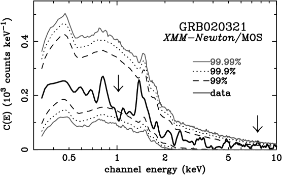
Figure 54: Same as in Figure 33 for GRB020321 MOS.

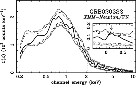
Figure 55: Same as in Figure 33 for GRB020322 PN.

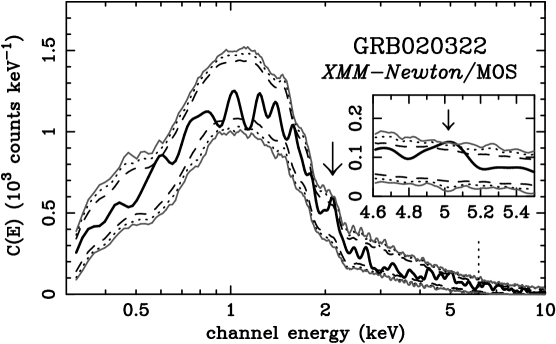
Figure 56: Same as in Figure 33 for GRB020322 MOS.

Figure 57: Same as in Figure 33 for GRB020405 zero order.

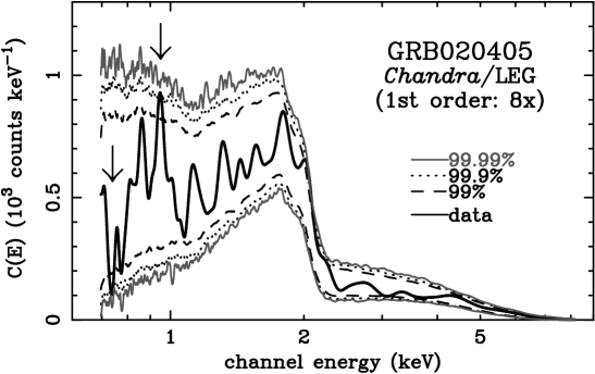
Figure 58: Same as in Figure 33 for GRB020405 dispersed.

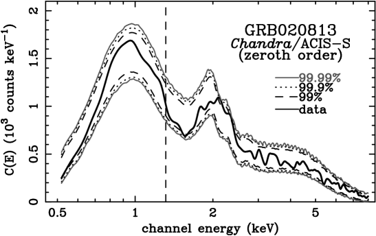
Figure 59: Same as in Figure 33 for GRB020813 zero order.

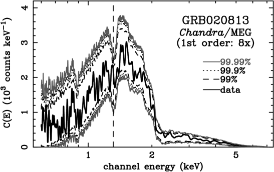
Figure 61: Same as in Figure 33 for GRB020813 MEG dispersed spectrum.

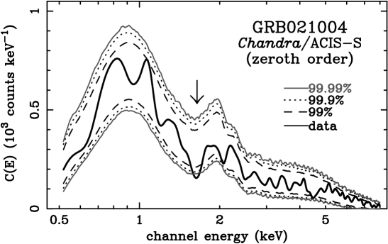
Figure 62: Same as in Figure 33 for GRB021004 zero order.

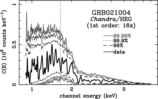
Figure 63: Same as in Figure 33 for GRB021004 HEG dispersed spectrum.

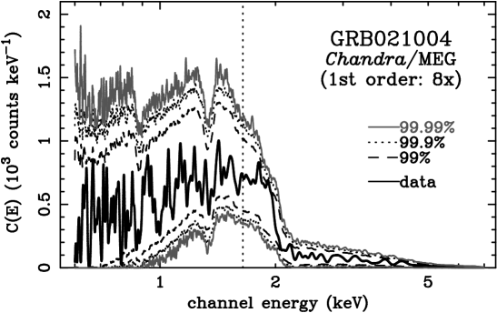
Figure 64: Same as in Figure 33 for GRB021004 MEG dispersed spectrum.

Figure 65: Same as in Figure 33 for GRB030226 ACIS.

Figure 73: Same as in Figure 33 for GRB030328 zero order.

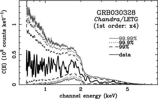
Figure 74: Same as in Figure 33 for GRB030328 LEG dispersed.

Figure 75: Same as in Figure 33 for GRB030329 PN time segment 1.

Figure 76: Same as in Figure 33 for GRB030329 MOS time segment 1.

Figure 77: Same as in Figure 33 for GRB030329 PN time segment 2.

Figure 78: Same as in Figure 33 for GRB030329 MOS time segment 2.

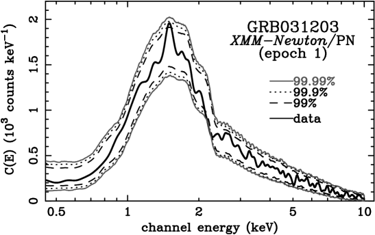
Figure 79: Same as in Figure 33 for GRB031203 PN time segment 1.

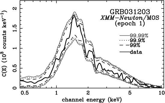
Figure 80: Same as in Figure 33 for GRB031203 MOS time segment 1.

Figure 81: Same as in Figure 33 for GRB031203 PN time segment 2.

Figure 82: Same as in Figure 33 for GRB031203 MOS time segment 2.

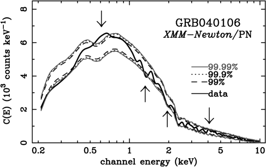
Figure 83: Same as in Figure 33 for GRB040106 PN.

References

- Altieri et al. (2000) Altieri, B., Schartel, N., Santos, M., Tomas, L., Guainazzi, M., Piro, L., & Parmar, A. 2000, GRB Circular Network, 869, 1
- Anders & Grevesse (1989) Anders, E. & Grevesse, N. 1989, Geochim. Cosmochim. Acta, 53, 197
- Ando et al. (2003) Ando, M., Ohta, K., Watanabe, C., Aoki, K., Ohyama, Y., Kawabata, K. S., Harasawa, S., Scarla, D., et al. 2003, GRB Circular Network, 1884, 1
- Antonelli et al. (2000) Antonelli, L. A., Piro, L., Vietri, M., Costa, E., Soffitta, P., Feroci, M., Amati, L., Frontera, F., et al. 2000, ApJ, 545, L39
- Ballantyne & Ramirez-Ruiz (2001) Ballantyne, D. R. & Ramirez-Ruiz, E. 2001, ApJ, 559, L83
- Barth et al. (2003) Barth, A. J., Sari, R., Cohen, M. H., Goodrich, R. W., Price, P. A., Fox, D. W., Bloom, J. S., Soderberg, A. M., et al. 2003, ApJ, 584, L47
- Berger et al. (2003a) Berger, E., Cowie, L. L., Kulkarni, S. R., Frail, D. A., Aussel, H., & Barger, A. J. 2003a, ApJ, 588, 99
- Berger et al. (2001) Berger, E., Frail, D. A., Price, P. A., Bloom, J. S., Galama, T. J., Kudritzki, R., & Bresolin, F. 2001, GRB Circular Network, 958, 1
- Berger et al. (2003b) Berger, E., Soderberg, A. M., Frail, D. A., & Kulkarni, S. R. 2003b, ApJ, 587, L5
- Bloom et al. (1998) Bloom, J. S., Djorgovski, S. G., Kulkarni, S. R., & Frail, D. A. 1998, ApJ, 507, L25
- Bloom et al. (2002) Bloom, J. S., Mirabal, N., Halpern, J. P., Fox, D. W., & Lopes, P. A. A. 2002, GRB Circular Network, 1294, 1
- Boella et al. (1997) Boella, G., Chiappetti, L., Conti, G., Cusumano, G., del Sordo, S., La Rosa, G., Maccarone, M. C., Mineo, T., et al. 1997, A&AS, 122, 327
- Boettcher (2003) Boettcher, M. 2003, ArXiv Astrophysics e-prints, astro-ph/0312538