New views of the solar wind with the Lambert W function

Abstract

This paper presents closed-form analytic solutions to two illustrative problems in solar physics that have been considered not solvable in this way previously. Both the outflow speed and the mass loss rate of the solar wind of plasma particles ejected by the Sun are derived analytically for certain illustrative approximations. The calculated radial dependence of the flow speed applies to both Parker’s isothermal solar wind equation and Bondi’s equation of spherical accretion. These problems involve the solution of transcendental equations containing products of variables and their logarithms. Such equations appear in many fields of physics and are solvable by use of the Lambert $W$ function, which is briefly described. This paper is an example of how new functions can be applied to existing problems.

American Journal of Physics, in press  (2004)

I Introduction

Most stars eject matter from their atmospheres and fill the surrounding space with hot, low-density gas.LC99 Astronomers and space physicists have studied the continuously expanding solar wind of charged particles from the Sun for almost a half century.Hu72 ; KR95 ; GP97 The study of the solar wind as a unique plasma laboratory is compelling for several reasons. Many basic processes in various fields of physics (for example, plasma physics, electromagnetic wave theory, and nonequilibrium thermodynamics) have been detected in the solar wind and almost nowhere else. The solar wind is the closest example of a stellar wind, and stellar winds affect the long-term evolution of galaxies by injecting large amounts of matter and energy into the interstellar medium. On the more practical side, when solar wind particles impact the Earth’s magnetosphere, they can interrupt communications, threaten satellites and the safety of orbiting astronauts, and disrupt ground-based power grids.SW01

The crown-like solar corona seen during a total eclipse is the place where the solar wind undergoes its initial acceleration. The shimmering auroras seen in northern and southern skies are the end products of the interaction between incoming solar wind particles and the Earth’s magnetic field. Sightings of the corona and the aurora go back into antiquity, but the first scientific understanding of the solar wind came at the beginning of the 20th century. Researchers gradually realized that there were strong correlations between the appearances of sunspot activity, geomagnetic storms, auroras, and motions in comet tails. In 1958, Eugene ParkerP58 ; P63 combined these empirical clues with the knowledge that the bright solar corona consists of extremely hot ($10^{6}$ K) plasma and postulated a model of a steady-state outward expansion from the Sun. Parker’s key insight was that the high temperature of the coronal plasma provides enough energy per particle to overcome gravity and produce a natural transition from a subsonic (bound, negative total energy) state near the Sun to a supersonic (outflowing, positive total energy) state in interplanetary space. This theory was controversial at the time, but Parker had only to wait four years until the existence of the continuous, supersonic solar wind was verified by the Mariner 2 probe in 1962.Hu72

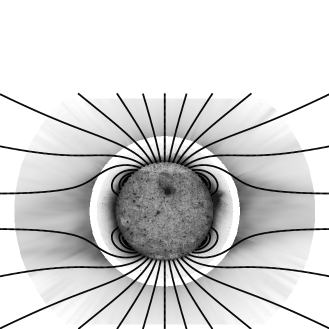
Figure 1: The solar corona on August 17, 1996, with bright regions plotted as dark. The inner image was taken by the EIT (Extreme-ultraviolet Imaging Telescope) instrument on Solar and Heliospheric Observatory (SOHO), and is sensitive to the ultraviolet emission of Fe⁺¹¹ ions at temperatures of about $10^{6}$ K. The outer image was taken by the UVCS (Ultraviolet Coronagraph Spectrometer) instrument on SOHO by blocking out the bright disk to see the much dimmer ultraviolet emission of O⁺⁵ ions at temperatures exceeding $10^{8}$ K. The magnetic field lines are from a model of the corona at the minimum of its 11-year activity cycle.Ba98

Over the past decade, our understanding of the physics of the solar wind has increased dramatically from both new space-based observations and the rapid growth of computer power for simulations (see Refs. Jk97, ; As01, ; Cr02, for recent reviews). The Ulysses spacecraft, for example, was the first probe to venture far from the ecliptic plane and soar over the solar poles to measure the solar wind in three dimensions.Ma01 Remote observations of the solar corona have become significantly more detailed with data from space-based telescopes pouring in as never before. Figure 1 shows a snapshot of the corona as observed in 1996 by two instruments on the SOHO (Solar and Heliospheric Observatory) spacecraft. However, progress in solar wind research often requires substantial numerical analysis, because even the most basic problems have not been tractable by analytic means. This paper takes advantage of a new transcendental function that is unfamiliar to many physicists—the Lambert $W$ function—to illustrate how two fundamental solar wind problems can be solved analytically.

In this era of efficient numerical computation, it is worthwhile to list the various ways that analytic solutions for the properties of the solar wind can be useful (beyond their pure aesthetic appeal). Analytic expressions often are used as initial guesses for more complicated iterative, time-dependent, or multi-dimensional calculations. Closed-form solutions also make it easier to study linearized perturbations to a known background state. The rapid evaluation of a large number of cases is facilitated by having analytic formulae, especially because many symbolic computation packages already contain optimized routines for the Lambert $W$ function. Finally, the ability to write down simple expressions for solar wind plasma properties may make the extrapolation to other stars more tractable and physically understandable.

This paper presents a brief overview of the Lambert $W$ function in Sec. II and a summary of the governing equations of the solar wind in Sec. III. The use of the $W$ function in solving the classical Parker solar wind problem, that is, the radial dependence of the wind speed for an isothermal plasma, is given in Sec. IV. The use of this function in solving for the mass loss rate of the solar wind is given in Sec. V. Conclusions and other potential applications of this function are given in Sec. VI.

II Some Properties of the Lambert W Function

Like many mathematical functions, the Lambert $W$ function was derived and used independently by several researchers before the mathematics and computer science community settled on a common notation in the mid-1990s.Co96 This function has been used to solve problems in electrostatics, statistical mechanics, general relativity, radiative transfer, quantum chromodynamics, combinatorial number theory, fuel consumption, and population growth,Co96 ; MO97 ; Ve00 ; Mg00 ; Ca03 but is still not widely known by physicists.

The Lambert $W$ function is defined as the multivalued inverse of the function $xe^{x}$. Equivalently, the multiple branches of $W$ are the multiple roots of the equation

$$W(z)e^{W(z)}=z,$$ (1)

where $z$ is in general complex. There are an infinite number of solution branches, labeled by convention by an integer subscript: $W_{k}(z)$, for $k=0,\pm 1,\pm 2,\ldots$ If $z$ is a real number $x$, the only two branches that take on real values are $W_{0}(x)$ and $W_{-1}(x)$. Figure 2 plots these two branches, which are the only ones that are needed in the applications of this paper.

Numerous formulae for the differentiation, integration, and series expansion of $W$ are given in the references cited above (for example, Ref. Co96, ; Ve00, ). One useful result, which is applied in the following, is given here. Near the branch cut point at $x=-1/e$, $W_{0}=W_{-1}=-1$, and the two real branches can be approximated to lowest order by

$$W_{0}(x) \approx -1+\sqrt{2+2ex}$$ (2)

$$W_{-1}(x) \approx -1-\sqrt{2+2ex}.$$ (3)

A useful way for expressing the solutions to a standard family of transcendental equations in terms of the Lambert $W$ function is to note that the equationBr98

$$\ln(A+Bx)+Cx=\ln D,$$ (4)

where $A$, $B$, $C$, and $D$ do not depend on $x$, has the exact solution

$$x=\frac{1}{C}W\Big{[}\frac{CD}{B}\exp\big{(}\frac{AC}{B}\big{)}\Big{]}-\frac{A}{B}.$$ (5)

The choice of solution branch usually depends on physical arguments or boundary conditions.

III Governing Equations of the Solar Wind

The expansion of the solar wind is treated traditionally as a problem of steady-state hydrodynamics. The Sun has a strong magnetic field that confines and directs the flow of plasma (see Fig. 1), but along the magnetic “flux tubes,” the dynamics is essentially independent of the strength of the field. Thus, the overall properties of the solar wind can be determined by solving the hydrodynamic equations of mass, momentum, and energy conservation.Hu72 ; LL87

The equation of mass conservation for a single-component fluid is given by

$$\frac{\partial\rho}{\partial t}+\nabla\cdot(\rho{\bf u})=0,$$ (6)

where $\rho$ is the mass density and ${\bf u}$ is the velocity. The equation of momentum conservation is

$$\frac{\partial{\bf u}}{\partial t}+({\bf u}\cdot\nabla){\bf u}=-\frac{1}{\rho}\nabla P+{\bf g},$$ (7)

where $P$ is the gas pressure and ${\bf g}$ is the net external force on a parcel of gas, here assumed to be only due to gravity. The equation of total energy conservation,

$$\frac{\partial}{\partial t}\big{(}\frac{\rho u^{2}}{2}+\frac{3P}{2}\big{)}+\nabla\cdot\Big{[}{\bf F}_{H}+{\bf F}_{C}+\rho{\bf u}\big{(}\frac{u^{2}}{2}+\frac{5P}{2\rho}-\frac{GM_{\odot}}{r}\big{)}\Big{]}=-\rho^{2}\Phi(T),$$ (8)

contains several terms that arise from the ionized nature of the near-Sun plasma. The solar corona exhibits a temperature of about $10^{6}$ K, which is at least two orders of magnitude higher than the temperature at the base of the atmosphere (that is, the photosphere and chromosphere). A major unsolved problem of solar physics is to explain what physical processes lead to such large amounts of energy into the coronal plasma. Significant progress has been made, though, by constraining the input energy flux density ${\bf F}_{H}$ empirically, even though the exact physical origin of this heating is not known.

Some of the energy deposited into the corona is transported downward to the lower atmosphere via heat conduction (that is, the radial component of ${\bf F}_{C}$ is negative), and some of it is converted back and forth between kinetic energy, thermal energy, and gravitational potential energy. (See the final three terms in square brackets in Eq. (8), where $G$ is the gravitational constant and $M_{\odot}$ is the mass of the Sun.) Some of this energy also is lost in the form of radiation, because many of the free electrons that exist in an ionized plasma undergo collisions with bound atoms and liberate a fraction of their energy to photon emission. The radiative loss function $\Phi(T)$ encapsulates the elemental composition and atomic physics of the radiating coronal plasma as a function of temperature $T$.

Equations (6)–(8) can be simplified in several ways without sacrificing realism. We can neglect the partial time derivatives and restrict our analysis to time-steady solutions of a continuously expanding solar wind. Also, the vector terms can be expressed in spherical polar coordinates, assuming that the variations exist only along the radial direction $r$ and that all vectors have nonzero components only in this direction. For example, the radial component of the gravitational acceleration ${\bf g}$ is simply $g_{r}=-GM_{\odot}/r^{2}$.

Very near the Sun, the assumption of radial flow is not accurate because of the complex multipole structure of the solar magnetic field (see Fig. 1). At larger distances, though, the radial flow of the solar wind has been largely confirmed by spacecraft measurements.Hu72 ; Jk97 However, the Sun’s slow rotation (once every 27 days) causes the flow direction and the magnetic field direction to become misaligned in interplanetary space. Because of the high conductivity of the solar wind plasma, the magnetic field lines become “frozen in” to the flow, that is, the magnetic field becomes a passive tracer of the flow, like drops of ink in a flow of water. A possible outdoor demonstration of this effect can be performed with a persistent, rotating source of water flow, like a lawn sprinkler. Despite the fact that all of the water droplets are flowing radially away from the center, a snapshot at any time shows them arranged in a spiral “streakline.” This field is completely analogous to the Parker spiral magnetic field pattern in the solar wind, which carries the imprint of the Sun’s rotation, but still channels the particle flow to be radial.

For the useful assumption of radial flow, the mass conservation equation is expressed in spherical symmetry as

$$\frac{1}{r^{2}}\frac{d}{dr}(\rho ur^{2})=0.$$ (9)

Because the radial derivative of $\rho ur^{2}$ is zero, this quantity is constant. We thus define the total mass loss rate from the entire Sun (in units of kg s^-1) as $\dot{M}\equiv 4\pi\rho ur^{2}$, where the factor of $4\pi$ comes from integrating over the full solid angle of the spherical Sun. The energy conservation equation is written as

$$\frac{1}{r^{2}}\frac{d}{dr}\Big{\{}r^{2}\big{[}F_{H}+F_{C}+\rho u\big{(}\frac{u^{2}}{2}+\frac{5P}{2\rho}-\frac{GM_{\odot}}{r}\big{)}\big{]}\Big{\}}=-\rho^{2}\Phi(T),$$ (10)

with the radial components of vectors written as scalars with the same notation.

The gas pressure $P$ can be eliminated from the momentum equation by applying the ideal gas law, assuming the fluid consists of a single particle species with mass $m$,

$$P=\frac{\rho kT}{m}\equiv\rho a^{2},$$ (11)

where $k$ is Boltzmann’s constant and $a$ is an effective sound speed. For a hydrogen plasma, $m$ is essentially the proton mass. An added assumption that simplifies the subsequent analysis is that the hot corona is isothermal, that is, that after the coronal heating takes hold, the $\sim$10⁶ K temperature remains roughly constant as a function of radius. It is known from spacecraft measurements that the plasma temperature drops only by a factor of 10 from the inner corona ($r\approx 1.5\,R_{\odot}$) to the orbit of the Earth ($r\approx 215R_{\odot}=1$ AU), where $R_{\odot}$ is the solar radius.Hu72 Therefore, for the acceleration region of the solar wind (1.5 to $10R_{\odot}$), the isothermal approximation seems sufficiently valid.

If we substitute these conditions into Eq. (7) and use the mass conservation equation, we obtain

$$\big{(}u-\frac{a^{2}}{u}\big{)}\frac{du}{dr}=\frac{2a^{2}}{r}-\frac{GM_{\odot}}{r^{2}}.$$ (12)

It is noteworthy that the momentum conservation equation is now a true equation of motion because the mass density $\rho$ no longer appears.

IV The Parker Solar Wind Problem

The fluid in a steady-state stellar wind accelerates from rest to an asymptotic “coasting” speed far from the star, where the star’s gravity has become negligible. This situation can only be maintained by a gradual transition from a hydrostatic force balance close to the star (that is, where inward and outward forces cancel) to a net outward force at larger distances.Vinf ParkerP58 recognized that this transition occurs naturally for a hot (million K) corona, where the gradient of the large gas pressure plays the role of the increasing outward force. Equation (12) shows the primary manifestation of the gas pressure gradient as the first term on the right-hand side, which for a constant $a$ eventually must overtake the more steeply decreasing gravity term and result in a net positive (outward) acceleration. Interestingly, the dynamics described by Eq. (12) does not depend on how the corona is heated, but merely on the fact that it is heated.

Parker also noticed that Eq. (12) exhibits a potential singularity at the “sonic point,” $u=a$, because when this condition applies, the term in parentheses on the left-hand side is zero, and for an arbitrary radius (that is, a finite value for the right-hand side) the first derivative of the velocity $du/dr$ must be infinite. However, there is one specific value for $r$ where the right-hand side is zero as well. If the sonic point occurs at the critical radius $r_{c}=GM_{\odot}/(2a^{2})$, then $du/dr$ may remain finite and the wind solution remains physically realistic. Mathematically, this solution represents an X-type singular point, at which two solution trajectories in $(r,u)$ space intersect with slopes of opposite signs and other solutions are hyperbolic about this point. The joint set of conditions $r=r_{c}$ and $u=a$ often is called the Parker critical point.

There are two possible solutions that pass through the critical point: one representing a continuously accelerating outward flow of gas (the wind), and one representing an outwardly decelerating, but inward flow of gas (steady spherical accretion). Parker’s wind solution was criticized initially for being too “finely tuned” because it seemed unlikely that a wind would naturally want to accelerate through the sonic point exactly at $r=r_{c}$. However, it has been noticed recently that Parker’s critical solution is the only truly stable wind solution to Eq. (12), and all other outwardly flowing solutions are unstable.Ve01 Note that six years before Parker, BondiBo52 recognized that the inward accretion solution also could represent real astrophysical flows. It was also found that this solution, like Parker’s, is a stable attractor and represents the maximum amount of mass that can be consumed (in steady state) from an external source.Ch90

Equation (12) is a first-order ordinary differential equation that is separable. The integration of the left side from $a$ to an arbitrary $u$ and the right side from $r_{c}$ to an arbitrary $r$ yields an implicit transcendental equation for $u$ and $r$:

$$(u^{2}-a^{2})-a^{2}\ln\big{(}\frac{u^{2}}{a^{2}}\big{)}=4a^{2}\ln\big{(}\frac{r}{r_{c}}\big{)}+2GM_{\odot}\Big{(}\frac{1}{r}-\frac{1}{r_{c}}\Big{)}.$$ (13)

We rearrange terms and define the dimensionless variable $y\equiv(u/a)^{2}$, so that Eq. (13) becomes

$$\ln y-y=\ln D(r),$$ (14)

where

$$D(r)=\big{(}\frac{r}{r_{c}}\big{)}^{-4}\exp\big{[}4\big{(}1-\frac{r_{c}}{r}\big{)}-1\big{]}.$$ (15)

Thus, using Eqs. (4) and (5), the Parker/Bondi solutions have the general analytic solution $y=-W[-D(r)]$. For all values of $r$, $D(r)$ ranges between 0 and $1/e$, so we must choose between the two branches $W_{0}$ and $W_{-1}$ (see Fig. 2). Additionally, the full solution involves one choice below the critical point and the opposite choice above it. The accelerating Parker solar wind solution is given specifically by

$$u^{2}=\begin{cases}-a^{2}W_{0}[-D(r)]&\text{$r\leq r_{c}$}\\ -a^{2}W_{-1}[-D(r)]&\text{$r\geq r_{c}$}\end{cases}$$ (16)

and the opposite choices must be made to obtain the Bondi accretion solution.

Figure 3 shows a set of solutions for the Parker solar wind with six choices for the constant sound speed $a$. These solutions are compared to curves showing empirical (that is, observationally derived) speeds for the fastest and slowest types of solar wind flow that have been seen. Because our only direct measurements of the wind speed have been exterior to the orbit of Mercury ($r>60R_{\odot}$), indirect methods are needed to determine the wind speed at distances closer to the Sun. The analysis of ultraviolet photons emitted from the corona has provided new ways of probing the solar wind’s acceleration,Cr02 but a more traditional method is to measure the density of particles in the corona and use mass conservation, that is, the steady state version of Eq. (9), to compute the wind speed. The density can be measured by observing the linear polarization of Thomson-scattered visible light in the corona; the degree of polarization is directly proportional to the number of free electrons along the line of sight.

In the following we give a simple parameterizationSG99 of the radial dependence of density as observed in the source regions of the fast and slow components of the solar wind (at the minimum of the Sun’s 11-year magnetic cycle):

$$\rho\,\mbox{(fast)} \approx 2.37\times 10^{-19}\big{(}\frac{1}{x^{2}}+\frac{5.9}{x^{3}}+\frac{650}{x^{9}}\big{)}\,\mbox{g}/\mbox{cm}^{3}$$ (17a)

$$\rho\,\mbox{(slow)} \approx 6.21\times 10^{-19}\big{(}\frac{1}{x^{2}}+\frac{13}{x^{3}}+\frac{480}{x^{6}}\big{)}\,\mbox{g}/\mbox{cm}^{3},$$ (17b)

where $x=r/R_{\odot}$. The wind speed at any radius is thus proportional to $\rho^{-1}r^{-2}$ times a normalization constant that is given by specifying the measured wind speed at 1 AU. Note that at large distances the dominant terms in Eq. (17) will be the $1/x^{2}$ terms, and thus $u\propto\rho^{-1}r^{-2}$ at large distances will approach a constant coasting speed.

The density is generally higher in the slower component of the solar wind, which emerges mainly from bright “streamers” around the solar equator and reaches speeds at 1 AU of 300 to 500 km/s. The density is lowest in the fast solar wind that emerges mainly from dark “coronal holes” at the north and south poles and reaches speeds at 1 AU of 600 to 800 km/s.Ma01 Figure 3 shows that the acceleration of the slow wind has a very similar shape to the analytic solutions given in Eq. (16). The fast wind has a slightly steeper profile in the corona because this plasma is not isothermal, and because it also flows slightly “super-radially” (that is, the magnetic field over the poles flares out like a trumpet and the equations are not represented exactly by spherical symmetry; see Fig. 1). However, much of the essential physics of solar wind acceleration remains encapsulated in the radial, isothermal problem.

One practical benefit of having an analytic expression for $u(r)$ is being able to easily find asymptotic expansions for various limiting cases. In the nearby vicinity of the critical point, that is, for $|1-(r_{c}/r)|\ll 1$, the series expansions given by Eqs. (2) and (3) can be used in conjunction with the series expansion of $D(r)$ about the critical point to obtain a single expression for radii near $r_{c}$:

$$u\approx a\,\sqrt{3-\frac{2r_{c}}{r}},\qquad\mbox{when}\ r\approx r_{c}.$$ (18)

Other expansions can be used to obtain approximations for $r\ll r_{c}$ and $r\gg r_{c}$.

V The Mass Flux Problem

The above solution (Eq. [16]) for the solar wind speed $u(r)$ is only half of the problem. Because the mass density $\rho$ was eliminated from the equation of motion, we know how fast the gas is accelerating, but we do not know how much gas is being ejected. The determination of the solar wind mass loss rate $\dot{M}$ is the second half of the problem which, interestingly, also is addressable using the Lambert $W$ function.

The Sun is observed to lose mass at a rate of approximately $10^{-14}$ solar masses per year ($M_{\odot}$/yr). This unconventional unit is useful because it can be compared easily to a firm upper limit derivable by dividing the mass of the star by its lifetime. For the Sun, with an expected main-sequence lifetime of about $10^{10}$ years, this upper limit is of order $10^{-10}\,M_{\odot}$/yr. Thus, the solar wind is expected to drain away no more than one ten-thousandth of the Sun’s mass over the next few billion years. (Some hotter stars lose mass at much higher rates, with the wind having a substantial impact on the star’s late stages of evolution.LC99 )

There is still not universal agreement about what determines the Sun’s mass loss rate.Ha82 ; Wi88 ; LM99 ; Fi03 Our analytic solutions apply to only one of the several suggested mechanisms. In this class of radiative energy balance models, first outlined in detail by Hammer,Ha82 $\dot{M}$ is determined at the base of the corona by the interplay between the heating and cooling terms in Eq. (10), the equation of energy conservation. Because we have solved for $u(r)$, the determination of the mass loss rate requires only the solution for the density at a single radius.

To simplify Eq. (10) further, the solar atmosphere can be considered to consist of two concentric layers: the cool ($\sim$10⁴ K), high density chromosphere, and the overlying hot ($\sim$10⁶ K), low density corona. The transition between these layers has been observed to be exceedingly thin—about 0.1% of a solar radius—so that the radial derivative in Eq. (10) can be expressed as a simple difference of quantities above and below the transition zone. Because of the relative thinness of this zone, we can ignore both the small change in the gravitational potential energy between the two layers and the spherical divergence, that is, the $r^{2}$ terms inside and outside the braces. Also, the kinetic energy term $u^{2}/2$ can be ignored because the solar wind speed has been seen to be negligibly small (that is, very subsonic) at the solar surface. Finally, the coronal heating term itself, $F_{H}$, is ignorable because we are concerned with layers below where the majority of the heat is deposited. Thus there are only three dominant terms in the energy balance:

$$\frac{d}{dr}(F_{C}+5nukT)=-\rho^{2}\Phi(T),$$ (19)

where for convenience we rewrite the mass density $\rho$ as the product of the particle mass $m$ and a number density $n$, that is, number of particles per unit volume. In summary, at the coronal base the heat is conducted downward from where it is initially deposited, some of it resides at the base as enthalpy, and the remainder is lost as radiation.

The steady state balance of mass and momentum across the thin transition zone also demands that the products $nu$ (mass flux) and $nT$ (gas pressure) remain roughly constant. This mass flux constraint is used, together with an empirical formRTV ; Wa94 for the radiative loss function $\rho^{2}\Phi\equiv n^{2}AT^{-1/2}$ (where $A=1.9\times 10^{-32}$ W m³ K^1/2), to obtain

$$\frac{dF_{C}}{dr}+5nuk\frac{dT}{dr}=-An^{2}T^{-1/2}.$$ (20)

The differential equation (20) is transformed by multiplying both sides by the heat conductive flux $F_{C}$. Note, though, that it is advantageous to multiply the left-hand side by $F_{C}$ itself and to multiply the right-hand side by the definition of the classical conductive flux,

$$F_{C}\equiv-\kappa T^{5/2}\frac{dT}{dr},$$ (21)

where $\kappa$ is the Spitzer-HärmSp62 heat conductivity in an ionized plasma, which has a value of $8.8\times 10^{-12}$ W m^-1 K^-7/2 for the range of densities and temperatures of the corona. We rearrange and divide all terms by a factor of $dT/dr$ and obtain the following form of the energy balance equation:

$$\xi F_{C}+F_{C}\frac{dF_{C}}{dT}=\psi,$$ (22)

where the quantities $\xi=5nuk$ and $\psi=n^{2}\kappa AT^{2}$ are assumed to be constant across the thin transition zone.

The above form (Eq. [22]) of the energy equation is separable and integrable with $T$ and $F_{C}$ as the independent and dependent variables, respectively. Once integrated across the transition zone, though, the full equation contains terms for $T$ and $F_{C}$ in both the upper and lower layers. The terms corresponding to the lower (chromospheric) layer can be neglected because the values of both $T$ and $F_{C}$ are several orders of magnitude smaller in comparison to their counterparts in the upper (coronal) layer. Thus, the integrated transcendental equation relates the values of $T$ and $F_{C}$ at the coronal base to one another and is independent of their values in the chromosphere:

$$F_{C}+\xi T+\frac{\psi}{\xi}\ln\big{(}1-\frac{\xi F_{C}}{\psi}\big{)}=0.$$ (23)

We note that both $\xi$ and $\psi$ contain the number density at the coronal base (which we call $n_{0}$). Hence, the Lambert $W$ function can be used to solve for this quantity, with

$$n_{0}=\frac{5u_{0}kF_{C}}{\kappa AT^{2}[1+W(\omega)]}$$ (24)

and the argument $\omega$ of the $W$ function is

$$\omega=-\exp\big{(}-\frac{25u_{0}^{2}k^{2}}{\kappa AT}\big{)}-1.$$ (25)

In this formulation, the only “free” variables are $u_{0}$, $F_{C}$, and $T$ (all evaluated at the coronal base). Just as in the Parker solar wind application, the argument $\omega$ falls between $-1/e$ and 0, thus making the choice between the $W_{0}$ and $W_{-1}$ branches necessary. In this case, though, the physical choice ($W_{-1}$) is apparent because the $W_{0}$ branch gives a negative density.

To use the above solution (Eq. [24]) to compute the mass loss rate, we use the results of Sec. IV to fix $u_{0}$ for a given isothermal Parker wind model. A realistic median value of $T$ is $1.2\times 10^{6}$ K, which has an outflow speed $u_{0}$ of 0.96 km/s at $r=R_{\odot}$. To estimate the applicable values of $F_{C}$ at the coronal base, Eq. (21) can be solved assuming a finite-difference temperature gradient across the thin transition zone. A thickness $\Delta r$ of 0.001 $R_{\odot}$ gives values of $F_{C}$ of order –1000 W m^-2. In more accurate models,Wa94 though, the temperature gradient is a bit less steep at the top of the transition zone, and $F_{C}$ ranges between –50 and –200 W m^-2. For this range, Eq. (24) for $n_{0}$ yields values of the number density between $6\times 10^{13}$ and $3\times 10^{14}$  m^-3. The mass flux, integrated around the whole sphere, is then $\dot{M}\equiv 4\pi m_{p}n_{0}u_{0}R_{\odot}^{2}$, and the resulting values range between $9\times 10^{-15}$ $M_{\odot}$/yr and $4\times 10^{-14}$ $M_{\odot}$/yr. The observed solar mass loss rate is observed to vary between about $2\times 10^{-14}$ $M_{\odot}$/yr at the solar minimum and a few times that at the solar maximum. If we take into consideration the large number of approximations we have applied, we conclude that the agreement is good.

VI Conclusions

We have presented new analytic solutions to two simple problems in solar wind physics. The Lambert $W$ function used in these solutions was defined and publicized only about a decade ago, but it has rapidly become a convenient tool for mathematical physicists. The elegance of explicit solutions to equations thought previously to be expressible only implicitly is clear, but there also are many practical benefits to having explicit solutions as well.

There are other potential applications of the Lambert $W$ function in solar and space physics. A transcendental equation solvable in terms of $W$ arises in a calculation of the electric potential drop that exists between the Sun and the edge of the solar system.MV99 (An ionized plasma exhibits local charge neutrality because of electrostatic screening, but for solar wind particles in the Sun’s gravitational field this neutrality is possible only by setting up a radially varying electric field.) Functions with temperatures $T$ appearing both inside and outside exponents occur when calculating the energy distributions of solar photons (for example, the Planck blackbody function) and electrons in excited atoms (for example, the Saha ionization equation). The Lambert $W$ function can thus be used in a variety of ways when the need to solve for $T$ arises. Further applications are expected to clarify the physics of many types of systems.

Figure Captions

Figure 2: The two real branches of the Lambert $W$ function.

Figure 3: Analytic solutions of the isothermal Parker solar wind equation, plotted as outflow speeds versus heliocentric distance (in units of a solar radius; $R_{\odot}=6.96\times 10^{8}$ m). Individual solutions (thin solid lines) are labeled with the locations of the critical point (circles). From bottom to top, the modeled coronal temperatures are 0.1, 0.2, 0.5, 1, 2, 5 MK, respectively. Shown for comparison are observationally constrained wind speeds for polar (thick dashed line) and equatorial (thick dotted line) flow at solar minimum.