Emission of CO, C i, and C ii in W3 Main

We used the KOSMA 3m telescope to map the core $7^{\prime}\times 5^{\prime}$ of the Galactic massive star forming region W3 Main in the two fine structure lines of atomic carbon and four mid-$J$ transitions of CO and ¹³CO. The maps are centered on the luminous infrared source IRS 5 for which we obtained ISO/LWS data comprising four high-$J$ CO transitions, [C ii], and [O i] at $63$ and $145\,\mu$m. In combination with a KAO map of integrated line intensities of [C ii] (Howe et al. 1991), this data set allows to study the physical structure of the molecular cloud interface regions where the occurence of carbon is believed to change from C⁺ to C⁰, and to CO. The molecular gas in W3 Main is warmed by the far ultraviolet (FUV) field created by more than a dozen OB stars. Detailed modelling shows that most of the observed line intensity ratios and absolute intensities are consistent with a clumpy photon dominated region (PDR) of a few hundred unresolved clumps per 0.84 pc beam, filling between 3 and 9% of the volume, with a typical clump radius of 0.025 pc ($2.2^{\prime\prime}$), and typical mass of 0.44 M_⊙. The high-excitation lines of CO stem from a $100-200$ K layer, as also the [C i] lines. The bulk of the gas mass is however at lower temperatures.

Table 1: List of observational parameters. The columns give line frequency, main beam efficieny $B_{\mathrm{eff}}$, half power beam width, obsering mode, number of mapped positions, velocity channel width $\Delta$v (the resolution is a factor of $\sim 1.4$ larger) , mean atmospheric zenith opacity $\langle\tau^{\mathrm{atm}}_{0}\rangle$, and observing period. The forward efficiency $F_{\mathrm{eff}}$ from skydips is constant at 0.9.

Species	Transition	Frequency	$B_{\mathrm{eff}}^{\mathrm{{\it c}}}$	HPBWc	Mode	Pos.	$\Delta$v	$\langle\tau^{\mathrm{atm}}_{0}\rangle$	Observing period
		[GHz]		[′′]			[m s-1]
12CO	$J=3{-}2$	345.7960	0.65	76	OTFa	1091	29	0.54	11/2000
13CO	$J=3{-}2$	330.5880	0.65	76	OTF	1091	29	0.63	1/2001, 8/2002
12CO	$J=4{-}3$	461.0408	0.57	57	DBSb	192	675	1.09	10/2001
12CO	$J=7{-}6$	806.6518	0.25	42	DBS	192	389	1.15	12/2001
13CO	$J=8{-}7$	881.2728	0.38d	40d	DBS	60	356	0.89	1/2003
12[C i]	3P${}_{1}{-}^{3}$P0	492.1607	0.50	55	DBS	192	634	0.82	12/2001
12[C i]	3P${}_{2}{-}^{3}$P1	809.3420	0.25	42	DBS	192	388	1.10	12/2001

• OTF – On-The-Fly observing mode using an emission-free off position at $(42.5^{\prime},-25.7^{\prime})$

• DBS – Dual-Beam-Switch mode using the secondary mirror ($6^{\prime}$ throw in azimuth)

• The main beam efficiency and the HPBW were determined from cross scans of Jupiter.

• Data at 880 GHz were taken after an adjustment of the primary mirror following photogrammetric measurements by Miller et al. (2002). The beam efficiency at 880 GHz was extrapolated from new efficiencies taken at 810, 492, and 345 GHz using the Ruze formula, consistent with a surface accuracy of 25 $\mu$m rms. The HPBW was scaled using the width at 810 GHz.

1 Introduction

Photon Dominated Regions (PDRs) are surfaces of molecular clouds where heating and chemistry are dominated by FUV $(6\,{\rm eV}<h\nu<13.4\,{\rm eV})$ radiation. The photons can scatter deep into the molecular clouds due to their clumpy structure. A large fraction of the volume and mass is thus photon dominated (Tielens & Hollenbach 1985). While FIR continuum emission by dust is by far the major coolant, the gas cools mainly via the atomic fine structure lines of O i, C ii, C i, and the rotational CO lines (e.g. Kaufman et al. 1999). Carbon bearing species are thus of great importance. The occurrence of carbon with depth into the surfaces changes from C⁺ to C⁰ and -finally- to CO. [C ii], [C i] and mid-$J$ CO lines trace the outer layers of photon dominated molecular clumps. However, [C ii] emission also stems from H ii regions, H i clouds (i.e. the cold neutral medium (CNM) (Kulkarni & Heiles 1987; Wolfire et al. 1995)), and diffuse H ii regions (i.e. the warm ionized medium (WIM) (Heiles 1994)). In the context of PDRs, depending on the induced chemistry, the critical densities, and energy levels of their transitions, [O i], [C ii], [C i], and CO lines serve as probes to trace different temperature and density regimes. In particular the two fine structure lines of neutral atomic carbon at 492 and 809 GHz provide information on the intermediate regions between atomic and molecular gas while tracing two different physical regimes.

Few studies have so far tried to map the major cooling lines of C ii/C i/CO in individual regions to derive a coherent picture of the chemical, physical, and -using velocity resolved line profiles- dynamical structure of the emitting regions. The studies of the massive star forming regions S106 by Schneider et al. (2003, 2002) and Orion Molecular Cloud 1 by Mookerjea et al. (2003) and Yamamoto et al. (2001), as well as the study of the reflection nebula NGC 7023 by Gerin & Phillips (1998) show that a coherent picture is not easily found using standard, steady-state PDR models. Especially the large spatial extension of neutral carbon and the high abundance deep inside molecular clouds appears to be in contradiction with standard PDR models. This is also addressed by the [C i] vs. CO studies of Plume et al. (1994) in S 140, Oka et al. (2001) in DR15, Kamegai et al. (2003) in $\rho$ Ophiuchi, and Oka et al. (2004) in NGC 1333. In a study of the translucent cloud MCLD $123.5+24.9$, Bensch et al. (2003) find lower than expected [C i] intensities and [C i] to CO ratios. Kamegai et al. (2003) and Oka et al. (2004) argue that [C i] traces young evolutionary stages of cloud surfaces which is consistent with time-dependent model calculations (cf. also Störzer et al. 1997). Gerin & Phillips (1998) suggest that a second PDR deeper in the cloud explains the observed enhanced [C i]/[CO] ratios in NGC7023. The importance of the interclump medium, providing effective shielding of the CO in the embedded clumps, is discussed by Bensch et al. (2003).

To improve our understanding of PDRs in different sources with different geometries and different FUV radiation fields, we present here a study of W3 Main. As the major cooling lines with their bright transitions are particular important as tracers in external galaxies, proper and detailed understanding of their emission and the chemical and physical conditions of the originating gas is necessary as a firm basis for their interpretation.

The chain of giant H ii regions W3-W4-W5 lie at the edge of the Cas OB6 association and form part of the Perseus spiral arm. Heyer & Terebey (1998) combined large-scale CO 1–0 FCRAO maps with H i line emission and 21 cm continuum DRAO data (Normandeau et al. 1997) (cf. Read 1981), and IRAS HIRES images at simmilar angular resolutions of about $1^{\prime}$. W3 is associated with the W3 giant molecular cloud comprising more than $10^{5}$ M_⊙ at a distance of 2.3 kpc (Georgelin & Georgelin 1976). This distance will be used throughout this paper, though Imai et al. (2000) recently found indications for a distance of only 1.8 kpc. W3 Main is a well known site of high-mass star formation comprising several H ii regions (Tieftrunk et al. 1995, 1997, 1998b, 1998a). ISO/SWS and LWS spectroscopy of the compact H ii region W3 A (Peeters et al. 2002) reveals strong atomic emission lines. W3 A is associated with a luminous infrared source IRS 2, belonging to a cluster of infrared sources (IRS 1–7) found by Wynn-Williams et al. (1972); Richardson et al. (1989). The total luminosity of IRS 5 is estimated to be $2-5\,10^{5}$ L_⊙ (Werner et al. 1980; Thronson et al. 1980; Campbell et al. 1995). Ladd et al. (1993) observed the associated emission of dust in the submillimeter identifying three cores (SMS 1$-$3). NIR observations by Megeath et al. (1996) reveal that high-mass star formation is associated with the formation of a dense cluster of several dozens of low-mass stars.

Column densities of molecular gas were mapped by Tieftrunk et al. (1995) in millimetric C¹⁸O and C³⁴S lines and by Roberts et al. (1997) in ¹³CO and C¹⁸O $1-0$. The latter observation were conducted with BIMA and reveal six clumps with diameters between 0.1 and 0.3 pc (masses between 120 and 480 M_⊙) in the vicinity of IRS 5 and IRS 4. The denser and warmer molecular gas in the vicinity of IRS 5$-$IRS 4 was observed by Hasegawa et al. (1994) in CO $3-2$ and $6-5$.

As part of a larger study of dense, hot gas in Galactic star forming regions, Krügel et al. (1989) and Boreiko & Betz (1991) observed ¹²CO $7-6$ and ¹²CO, ¹³CO $9-8$ towards W3 IRS 5, respectively. The large-scale extent of the 492 GHz line of atomic carbon and of ¹³CO and C¹⁸O $2-1$ was observed by Plume et al. (1999) at $3^{\prime}$ resolution. Howe et al. (1991) mapped the [C ii] 158$\,\mu$m emission of W3 Main and developed models to reconcile the distribution of [C ii] emission and the FUV field.

Here, we attempt to model the mapped emission of mid-$J$ and high-$J$ CO lines, of both [C i] lines, and of [C ii], at resolutions of $\sim 1^{\prime}$. Section 2 describes the KOSMA observations and the ISO/LWS data set. Section 3 presents the maps of integrated intensities, spectra at four selected positions, and a first derivation of physical properties. In Sect. 4 we discuss the physical structure of the photon dominated regions. We present a model of the FUV field, needed for a detailed comparison of line integrated intensities with PDR models. We summarize our results in Sect. 5.

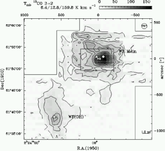
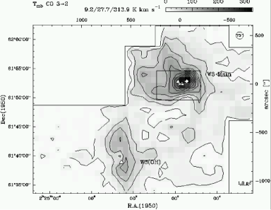
Figure 1: (Left) Integrated ¹³CO and (Right) ¹²CO $3{-}2$ large scale maps of W3, including W3 Main in the north and W3(OH) in the south. The integration interval is [$-55,-25\,\,\mathrm{km}\,\mathrm{s}^{-1}$] and thus also covers the emission of W3(OH). Offsets are given in arcsec. Contour levels are described in the upper left corner of each map: first contour$=3\,\sigma$/step size/peak intensity. The position $(0,0)$ of IRS 5 is marked by a star, IRS 4 is marked by a square. Triangles mark the positions of IRS 1 (to the east), IRS 3, and W3(OH). The inner black box indicates the size of the higher frequency maps shown below. The 0/0 position is at IRS 5: $\alpha{(1950)}=02\aas@@fstack{h}21\aas@@fstack{m}53\aas@@fstack{s}2$ $\delta{(1950)}=61\degr 52\arcmin 21\arcsec$.

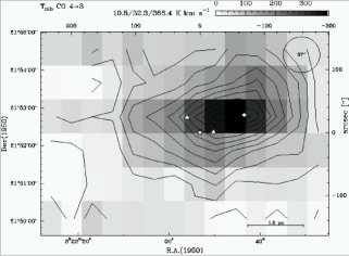
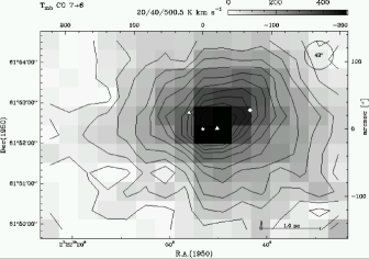
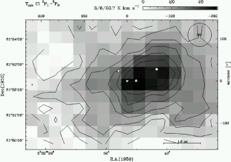
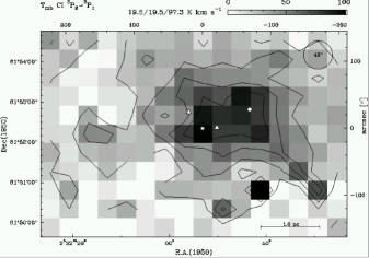
Figure 2: (From upper left to lower right) Integrated intensity maps of CO $4{-}3$, CO $7{-}6$, [C i] $1{-}0$ and [C i] $2{-}1$ of the W3 Main region (indicated by the rectangle in Figure 1).

Figure 3: Map of ¹³CO 8–7 spectra at a resolution of $75^{\prime\prime}$ (0.84 pc) and on the $T_{\rm mb}$ scale after a pointing correction. The temperature range is $-2$ to 10 K. The $v_{\rm lsr}$ range is $-70$ to $-10$ kms^-1.

2 Observations

The KOSMA 3m submillimeter telescope on Gornergrat, Switzerland (Winnewisser et al. 1986; Kramer et al. 1998, 2000) was used to observe the transitions of carbon and the mid-$J$ transitions of CO.

2.1 [C i] and mid-$J$ CO

We have mapped W3 (Fig. 1, 2) in the two atomic carbon fine structure transitions ([C i]) at 492 GHz (609 $\mu$m, ³P${}_{1}{-}^{3}$P₀; hereafter $1{-}0$) and 809 GHz (370 $\mu$m, ³P${}_{2}{-}^{3}$P₁; hereafter $2{-}1$) and the mid-$J$ rotational transitions $J=4{-}3$ and $J=7{-}6$ of CO, and $J=8{-}7$ of ¹³CO using the newly installed SubMillimeter Array Receiver for Two frequencies (SMART) (Graf et al. 2002) on KOSMA.

SMART is a dual-frequency eight-pixel SIS-heterodyne receiver that simultaneously observes in the 650 and 350 $\mu$m atmospheric windows (Graf et al. 2002). It consists of two 4 pixel subarrays, one operating in the frequency band of $455-495$ GHz and the other in the band of $795-882$ GHz. The IF signals are analyzed with two 4-channel array-acousto-optical spectrometers with a spectral resolution of 1.5 MHz (Horn et al. 1999). The IF frequency of 1.5 GHz is ideally suited for simultaneous detections of the [C i] $2{-}1$ line at 810 GHz and the CO $7{-}6$ line at 806 GHz in opposite sidebands. The two subarrays are pointed at the same positions on the sky. Thus, four spatial positions are observed simultaneously. The [C i] $1{-}0$ & $2{-}1$ and the CO $7{-}6$ observations of W3 presented here were done simultaneously. The relative pointing is thus constant. Due to the simultaneous observations at both frequency bands, relative calibration errors are strongly reduced and line ratios are measured precisely (cf. e.g. Stutzki et al. 1997). The typical receiver noise temperatures achieved at the center of the bandpass is around 150 K at 492 GHz and between 500 and 600 K at 810 GHz. The receiver setup consists of a K-mirror type image rotator, two Martin-Puplett diplexers, and two solid state local oscillators, which are multiplexed using collimating Fourier gratings (Graf et al. 2002). The image rotator corrects for the sky rotation during the observation and it allows to set the array to any desired orientation.

The observations were performed in Dual-Beam-Switch mode (DBS), with a chop throw of $6^{\prime}$ in azimuth. This mode of observation produces flat baselines. Only a zeroth order baseline was subtracted from the calibrated spectra. The spacing between two adjacent pixels is $114^{\prime\prime}$. Pointing was frequently checked on Jupiter and the sun. The resulting accuracy is better than $\pm 20^{\prime\prime}$.

An area of $\sim 7^{\prime}\times 5^{\prime}$ was mapped in the two [C i] lines and the two CO lines, on a $27.5\arcsec\times 27.5\arcsec$ grid with a total integration time of 160 s per position. Due to the extent of the W3 cloud complex weak self-chopping artefacts were found at the borders of the mapped region. This was confirmed by separate observations of these positions in total power position switch mode. We did not correct for these artefacts.

Atmospheric calibration was done by measuring the atmospheric emission at the OFF-position to derive the opacity (Hiyama 1998). Spectra of the two frequency bands near 492 and 810 GHz were calibrated separately. Sideband imbalances were corrected using standard atmospheric models (Cernicharo 1985). The CO $7{-}6$ line observed in the image sideband, was also corrected.

A small map of the ¹³CO 8–7 line at 880 GHz covers an area of $5.5^{\prime}\times 2.3^{\prime}$ centered on IRS 5 and IRS 4 (Fig. 3). Integration times are on average 480 sec per position. No self-chopping effects are discernable in the resulting spectra. A pointing offset was corrected off-line by shifting the ¹³CO data by ($0^{\prime\prime}$,$-27.5^{\prime\prime}$). The main beam efficiency $B_{\mathrm{eff}}$ and HPBWs were determined using continuum cross scans on Jupiter (Table 1). Griffin et al. (1986, Table 1) observed Jupiter and Mars at 10 frequencies in the $0.35$ to 3.3 mm wavelength range using Mars as primary standard. We used their Jovian brightness temperatures, linearily interpolated, to derive the temperatures at the frequencies of the KOSMA observations. The KOSMA half power beamwidths (HPBWs) were derived from the observed FWHMs. At 810 GHz $\sim 25$% of the emission is detected by the main beam. Continuum scans of the edge and disc of the sun reveal an extended Gaussian error beam component of $\sim 200^{\prime\prime}$ FWHM, detecting about $40\%$ of the emission. We attribute this error beam to residual misalignment of the $18$ panels of the primary mirror. Due to the large extent of the errorbeam relative to the mapped region, we cannot convolve out the errorbeam. Instead, we simply scaled the antenna temperature data with the ratio of forward over main beam efficiency to go from the $T_{A}^{*}$ scale to the $T_{\mathrm{mb}}$ scale.

From observations of reference sources, we estimate the relative calibration error to be $\sim 15\%$.

2.2 Low-J CO & ¹³CO

We have used a dual-channel SIS receiver (Graf et al. 1998) on KOSMA to observe large scale maps in CO $J=3{-}2$ and ¹³CO $3{-}2$ emission of W3 (Müller 2001). The observations were done using the On-The-Fly (OTF) technique (Beuther et al. 2000; Kramer et al. 2000) on a fully sampled grid of $30^{\prime}\times 30^{\prime}$. For the low-frequency observations we used the high resolution spectrometer (HRS1) till Winter 2001 and the variable resolution spectrometer (VRS1) lateron. Sinusoidal baselines were subtracted. See Table 1 for a summary of observational parameters.

2.3 ISO/LWS spectroscopic data

ISO/LWS (Clegg et al. 1996) spectra are available from the data archive for the position of IRS 5 in W3 Main (TDT 47301305). The grating spectrometer covers the wavelength range $47-197\,\mu$m. The standard OLP-10 data product was used along with ISAP v. 2.1 to deglitch, defringe, and average the data. Linear baselines were subtracted from all spectra. Gaussian fits, with the line width held fixed at the instrumental width, were done to derive integrated intensities.

3 Results

3.1 Why to use different tracers?

The observed transitions trace varying physical conditions of the emitting regions. Transitions are characterized by their critical density for collisions with H₂ or other partners and by their upper level energy (see Table 2 in Kaufman et al. 1999). For the CO $J\rightarrow{}J-1$ transition, the critical density is $4\,10^{3}\,J^{3}$ cm^-3 and the upper level energy corresponds to $2.8\,J(J+1)$ Kelvin. The mid-$J$ CO transitions observed with KOSMA are thus sensitive to gas at about $10^{5}$ to $10^{6}$  cm^-3 at temperatures between 30 and 200 K while the high-$J$ lines traced by ISO/LWS are sensitive to typically $10^{7}$ cm^-3 and 650 K. The regime of high densities $>10^{5}$ cm^-3 and high temperatures $>200\,$K is also traced by the two atomic [O i] lines at $145\,\mu$m and $63\,\mu$m. On the other hand, the two atomic [C i] lines and the [C ii] line trace energies of less than 100 K and densities of less than $3\,10^{3}$ cm^-3.

3.2 Maps of integrated intensities

We present here KOSMA maps of W3 Main at spatial resolutions of about one arcminute. The ¹²CO and ¹³CO $3-2$ maps include W3 Main and W3 (OH), and cover an area of $\sim 20^{\prime}\times 14^{\prime}$. A $7^{\prime}\times 5^{\prime}$ region centered in W3 Main-IRS5 was mapped in [C i] ³P${}_{1}-^{3}$P₀, ³P${}_{2}-^{3}$P₁, ¹²CO $4-3$, and $7-6$. The $5.5^{\prime}\times 2.3^{\prime}$ map of ¹³CO $8-7$ covers the IRS 5 and IRS 4 positions. We have included in our analysis the [C ii] map of Howe et al. (1991) and ISO/LWS data at the position of IRS 5.

In contrast to the velocity integrated CO maps which show only one maximum near IRS 5, the corresponding spectra show many details like self-absorption features and overlapping velocity components. These will be discussed in Sect. 3.3.

3.2.1 Maps of ¹²CO and ¹³CO $3-2$

The ¹²CO and ¹³CO $3{-}2$ maps exhibit ($i$) a single central peak close to the position of IRS 5, ($ii$) an extension to the north-east toward W3 North (cf. Plume et al. 1999), which is the northernmost member of the string of active star-forming regions, and ($iii$) a ridge of emission extending towards the south in the direction of W3 (OH). In addition, ($iv$) both maps show another ridge of emission extending eastward from IRS 5 and then bending north-east. The two north-eastern ridges are more clearly seen in the ¹³CO isotopomer than in ¹²CO.

3.2.2 Maps of CO $4-3$ and $7-6$

The higher-frequency maps cover the central part of W3 Main encompassing an area of $\sim 7^{\prime}\times 5^{\prime}$.

The CO $4-3$ and $7-6$ maps again show a strong peak near IRS 5, slightly shifted towards IRS 4, which drops rather steadily in all directions. A ridge of emission extending from IRS 4 in south-western direction is discernable in the CO $7-6$ data set.

3.2.3 Maps of [C i] $1-0$ and $2-1$

Comparison of the C i maps with the CO maps in Figures 1 and 2 shows that although there is a large-scale similarity between the two emission patterns, the mid-$J$ CO emission is more centrally concentrated than the [C i] emission. This indicates the origin of the CO emission in regions with high density and temperature, while the [C i] emission originates in regions of comparatively lower density and temperature, and hence traces out the widespread diffuse UV illuminated neutral gas.

3.3 Spectra at selected positions

In Figure 4, we present spectra at four positions, IRS 4, IRS 5, and two positions 0.92 pc ($85^{\prime\prime}$) to the north and to the south of IRS 5 where the line integrated intensities drop to about a third of the peak intensities. In general, ¹²CO line shapes show a complicated structure, espcially at IRS 5 and 4, while ¹³CO and [C i] line shapes show little deviations from Gaussian profiles.

At the position of IRS 5, the ¹²CO 3–2 and 4–3 spectra clearly show an absorption dip, while the ¹²CO 7–6 spectrum is flat-topped. The ¹³CO and [C i] spectra all peak at about the velocity of the dip, near $-38\,\,\mathrm{km}\,\mathrm{s}^{-1}$. The foreground absorption in the center region of W3 Main is already well known from the CO observations of Hasegawa et al. (1994). It is also seen in the water line observed with the Odin satellite (Wilson et al. 2003). In order to correct for self-absorption in the ¹²CO line profiles, we have fitted Gaussian profiles to the line wings (Fig. 4) to derive reconstructed integrated intensities and their ratios (Table 2). In the following, we will only use the corrected line integrated ¹²CO intensities.

The ¹²CO FWHM line widths at IRS 5 are $\sim 9\,\,\mathrm{km}\,\mathrm{s}^{-1}$, larger than those of the ¹³CO lines which are in turn larger than those of the [C i] lines which exhibit $\sim 6\,\,\mathrm{km}\,\mathrm{s}^{-1}$.

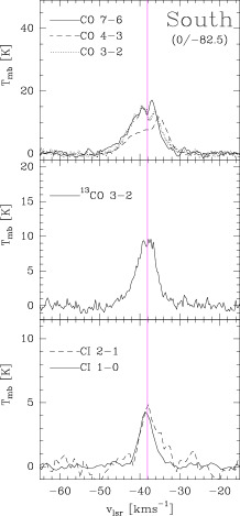
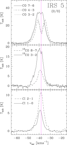
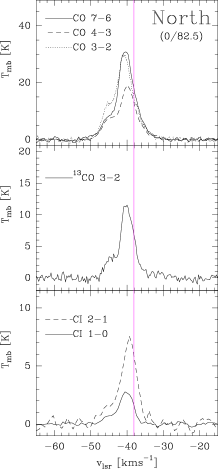
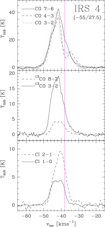
Figure 4: Spectra at four representative positions, including IRS 5 and IRS 4. All spectra are on a common spatial resolution of $75^{\prime\prime}$ (0.84 pc) and are plotted on the $T_{\rm mb}$ scale at 0.1 kms^-1 channel spacing. ¹³CO and [C i] lines peak at the velocity of a dip in the ¹²CO spectra, indicating that the dip is due to a colder foreground component at about $-38$ $\,\mathrm{km}\,\mathrm{s}^{-1}$ (denoted by a vertical line). To estimate the line integrated ¹²CO intensity of the background source, we fitted a Gaussian to the line wings of the ¹²CO spectra. Figure 5 gives an example.

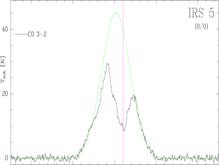
Figure 5: The ¹²CO 3–2 spectrum at IRS 5 is shown together with the Gaussian line profile fitted to the line wings. The ratio of fitted to observed line integrated intensity is 1.5. The lower box shows the residual of the profile fit.

3.4 Temperatures and carbon budget at four representative positions

Observed line integrated intensities at the same angular resolution of $75^{\prime\prime}$ and some derived line ratios are compiled in Tables 2 and 3. Physical parameters at the four selected positions are listed in Table 4.

3.4.1 CO line ratios, excitation temperatures, and beamfilling factors

The ¹²CO 7–6/¹²CO 4–3 line ratio of integrated intensities (Table 3), corrected for self-absorbed line profiles, varies between 1.0 and 1.3. This is consistent with optically thick emission. Assuming equal excitation temperatures (LTE), a ratio of $1\pm$20% indicates temperatures of more than 40 K. This is consistent within the errors with the excitation temperatures derived from ¹²CO 3–2 peak line temperatures in the center region and to the North, again assuming optically thick emission (Table 3). Excitation temperatures from CO 7–6 are $\sim 10\,$K higher due to the Rayleigh-Jeans correction at equal peak line temperatures.

Only the ISO/LWS observations of high-$J$ CO transitions at IRS 5 together with an escape probability analysis (Chapter 4.4.3) show that an additional gas component exists exhibiting temperatures of more than 140 K.

These arguments, assume so far that radiation is emitted from a homogeneous region. However, temperature and density gradients are known to exist in UV illuminated clouds. We will explore their significance when comparing the observations with PDR models in Sect. 4.5.

Table 2: Observed integrated intensities in $\mathrm{K}\,\mathrm{km}\,\mathrm{s}^{-1}$ at the four positions in W3 Main shown in Figure 4. The ¹²CO line intensities were corrected for self-absorption. For this reason, some of the integrated intensities are identical. The error on the integrated intensities observed with KOSMA is estimated to be $\sim 15\%$. [C ii] intensities are from Howe et al. (1991).

$\Delta\alpha/\Delta\delta$	12CO				13CO			[C i]			[C ii]
$[^{\prime\prime},^{\prime\prime}]$	3–2	4–3	7–6		3–2	8–7		3P${}_{1}{-}^{3}$P0	3P${}_{2}{-}^{3}$P1		2P${}_{3/2}{-}^{2}$P1/2
0,0 (IRS 5)	408.4	408.4	432.4		148.7	52.9		38.3	73.5		311.3
$-55.0/27.5$ (IRS 4)	408.4	408.4	432.4		158.6	37.4		42.5	78.2		267.2
0,82.5 (North)	231.2	231.2	231.2		63.7	–		15.5	44.3		148.8
$0,-82.5$ (South)	129.9	99.4	132.7		60.2	–		21.3	27.4		311.3

Table 3: Selected ratios of observed integrated intensities in $\mathrm{K}\,\mathrm{km}\,\mathrm{s}^{-1}$ at the four positions in W3 Main which are shown in Figure 4. The error on the integrated intensity ratios observed with KOSMA is estimated to be $\sim 20\%$. For comparision, we also list ratios observed in other sources by ^a Schneider et al. (2003, KOSMA), ^b Wilson et al. (2001, HHT), ^c Zhang et al. (2001, AST/RO), ^d Petitpas & Wilson (1998, JCMT), ^e Fixsen et al. (1999, COBE), ^f Stutzki et al. (1997, HHT), ^g Israel & Baas (2002, JCMT, Fig.2), ^h Yamamoto et al. (2001, Mt.Fuji), ⁱ Mao et al. (2000, HHT/IRAM 30m), ^k Weiss et al. (2003, IRAM PdBI), ^m Tieftrunk et al. (2001, AST/RO).

$\Delta\alpha/\Delta\delta$	12CO 3-2		CO 7-6		13CO 3-2		[C i] 2-1		[C i] 1-0		[C ii]		[C ii]
$[^{\prime\prime},^{\prime\prime}]$	13CO 3-2		CO 4-3		13CO 8-7		[C i] 1-0		CO 4-3		[C i] 1-0		CO 4-3
W3 Main:
0,0	2.75		1.06		2.81		1.92		0.09		8.14		1.12
$-55,28$	2.57		1.06		4.24		1.84		0.10		6.29		0.82
0,82.5	3.63		1.00		–		(2.86)		0.07		9.60		1.11
$0,-82.5$	2.16		1.33		–		1.29		0.21		14.62		3.27
S106a	3.0		1.03–1.57				1.0–1.8		0.12–0.38		6.4		0.8
Orion A			1.2–3.5b				0.83h
Carina MCc									0.14–0.45
G333.0-0.4, NGC6334A, G351.6-1.3							0.48-0.75m
Inner Galaxye									0.31		3.54		4.29
Galactic Centere			0.11						0.22		1.38		0.71
M83 Nucleusd									0.14–0.47
M82 Center			0.28-0.36i				1.0f
Sample of 15 galaxiesg									0.1–1.2
Cloverleaf							0.54k

Table 4: Physical parameters at four positions in W3 Main. The excitation temperature $T_{\rm ex}{\rm(CO)}$ (col. (1)) is derived from ¹²CO 3–2 peak temperature. Lower limits of the C i excitation temperature (col. (8)) are derived from the [C i] 2–1/1–0 line ratio assuming a calibration error of 20%. For the calculation of CI column densities, it was however assumed that $T_{\rm ex}$([C i]) is 100 K constant. Column densities per $75^{\prime\prime}$ beam (0.84 pc) and the relative abundances of the three major gas phase species CO, C i, and C ii, are derived assuming LTE (cf. chapter 3.5.1). The FUV field $G_{0}$ smoothed to $75^{\prime\prime}$ is estimated from the luminosity of the embedded OB stars (cf. chapter 4.1).

$\Delta\alpha/\Delta\delta$	$T_{\rm ex}$(CO)	$N$(CO)	$N$(C i)	$N$(C ii)	C i:CO	C ii:C i:CO	$T_{\rm ex}$(C i-Ratio)	$N$(H2)	$G_{0}$
$[^{\prime\prime},^{\prime\prime}]$	[K]	$[10^{17}$ cm${}^{-2}]$					[K]	$[10^{21}$ cm${}^{-2}]$	$[10^{4}]$
$0,0$	53.	55.2	5.8	13.8	10:90	18: 8:74	$>122$	39.9	40.4
$-55.0,27.5$	53.	58.7	6.4	11.8	10:90	15: 8:76	$>108$	42.5	19.9
$0,82.5$	39.	20.9	2.4	6.6	10:90	22: 8:70	–	15.1	10.4
$0,-82.5$	21.	26.2	3.2	13.8	11:89	32: 7:61	$>54$	18.9	6.7

3.4.2 [C i] line ratios

Ratios of the two [C i] lines vary systematically between 1.3 in the south and 2.9 in the north (Table 3). These ratios indicate optically thin emission since for optically thick [C i] lines we would expect line ratios of about 1 or less. The low peak line temperatures of less than 11 K do not reflect the kinetic temperatures estimated above, instead they also indicate low optical depths ($\tau<0.15$ for $T_{\rm ex}=100\,$K).

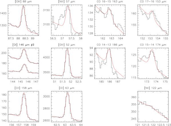
Figure 8: Individual ISO/LWS spectra at IRS 5/W3 Main (cf. Fig. 7). Drawn lines show the fitted instrumental line profiles. Integrated line intensities are listed in Table 6.

In the optically thin limit, the excitation temperature is a sensitive function of the line ratio $R$ in $\mathrm{K}\,\mathrm{km}\,\mathrm{s}^{-1}$: $T_{\mathrm{ex}}=38.8\,{\mathrm{K}}/\ln[2.11/R]$. In Column (8) of Table 4 we give the lower limit on $T_{\rm ex}$ using this formula given the observational error on the line ratio. The error is such that only lower limits on excitation temperatures can be derived. Ratios above 2.11 as found at one position north of IRS 5 lead to unphysical negative excitation temperatures. Detailed PDR modelling by Kaufman et al. (1999, Fig.8) confirms that for densities of upto $n=10^{7}$ cm^-3 and FUV fields of upto $G_{0}=10^{6.5}$ the CI line ratio stays below 2.1.

To exclude systematic observational errors, e.g. due to the KOSMA error beam at short wavelengths or due to the atmospheric calibration, we studied the distribution of all observed CI line ratios. In total 167 positions were observed, out of which 14 positions (8.4%) show a CI line ratio greater than 2. This is consistent with a true ratio of 1.5, a 20% $1\sigma$ error, and a Gaussian error distribution (e.g. Taylor 1982). Using the above simplifying formula for optically thin emission and equal $T_{\rm ex}$, a ratio of 1.5 results in a temperature of 114 K which is characteristic for the average temperature of the CI emitting gas.

In conclusion, carbon excitation temperatures derived from the [C i] line ratios are typically 100 K, and are higher than those derived from ¹²CO. However, the sensitivity of the above ansatz on the observational errors for high observed ratios does not allow more quantitative conclusions.

Only few observations of the upper [C i] line are reported so far (Table 3). The 809 GHz line was first detected by Jaffe et al. (1985) and later observed by Genzel et al. (1988) in M 17 and W 51. The COBE satellite observed the Milky Way at $8^{\circ}$ resolution and found low line ratios (Fixsen et al. 1999) of 0.31 in the inner Galactic disk, corresponding to a kinetic temperatures of $>20$ K. Line ratios observed in Orion A (OMC1) Yamamoto et al. (2001) using the Mt.Fuji telescope indicate excitation temperatures covering the range of 52 to 62 K and more. Zmuidzinas et al. (1988) detected the upper [C i] line in several Galactic star forming regions with the KAO, and derived excitation temperatures between 25 K and 77 K from the [C i] 2–1/1–0 line ratios. They derived a carbon excitation temperature of 25 K from observations of W3. This is in contradition to our result which is however based on simultaneous observations with the same instrument. Moreove data were smoothed to the same spatial resolution thus reducing possible calibration errors.

3.5 The case for hot gas at IRS 5

Helmich et al. (1994) found rotational temperatures of SO₂, CH₃OH, and H₂CO ranging between 64 and 187 K when using the JCMT with high spatial resolutions. van der Tak et al. (2000) find rotational temperatures of CH₃OH and H₂CO of 73 and 78 K.

High-$J$ lines of CO and ¹³CO $v=0-1$ (4.7 $\mu$m) absorption measurements towards IRS 5 with a subarcsecond sized beam given by the size of the IR continuum background source (Mitchell et al. 1990, at the CFHT) reveal a hot gas component at 577 K comprising $\sim 50\%$ of the total gas column density per beam at densities exceeding $10^{7}$ cm^-3. A colder component at $\sim 66$ K comprises the other half.

Solid CO is also detected towards IRS 5 (Sandford et al. 1988; Lacy et al. 1984; Geballe 1986), but contributes only 0.2 % to the total CO column density (Mitchell et al. 1990). ISO-SWS observations of the ¹³CO₂ ice band profile (Boogert et al. 2000) towards IRS 5 show indications of heated ice, consistent with the above results.

Ammonia observations at resolutions of $40^{\prime\prime}$ were used by Tieftrunk et al. (1998b) to derive kinetic temperatures at the positions of IRS 5 and 4. While the kinetic temperature at IRS 4 is estimated to be 48 K in excellent agreement with the excitation temperature we have derived from ¹²CO 3–2, the kinetic temperature at IRS 5 was estimated to be 150 K.

In conclusion, observations indicate a strong temperature gradient peaking at IRS 5 at upto 600 K. The hot gas component has a low beam filling factor while the colder gas component is more widespread. Variations of optical depths and chemistry are also at play.

3.5.1 Relative carbon abundances

Table 4 lists the relative abundances of the major carbon bearing species in the gas phase: C ii, C i, and CO. These are derived from column densities assuming optical thin ¹³CO 3–2, [C i], and [C ii] emission and LTE. For the C i column density we assumed an excitation temperature of 100 K at all positions. Note that the column density is not temperature sensitive: an increase of $T_{\rm ex}$ by a factor of 2 only results in a 10% increase of the column density. C ii column densities are independent of the excitation temperature in the thermalized limit and for temperatures much higher than 91 K (see e.g. Schneider et al. 2003).

The total H₂ column density is derived from the ¹³CO 3-2 integrated intensity via the CO column density assuming a ¹²CO/¹³CO abundance of 65 (Langer & Penzias 1990) and a H₂/CO abundance of $8\,10^{-5}$.

In W3 Main, the relative abundances of C i/CO are rather constant: the ratio is $\sim 0.11$ at all four positions. Similar ratios of $\sim 0.1$ are found by Zmuidzinas et al. (1988) in a study of seven Galactic star forming regions. Plume et al. (2000) derive similar CI/CO ratios in the Orion A cloud, but observed an increase towards the cloud edges to values of $\sim 0.5$. Schneider et al. (2003) find low ratios in S 106 varying between 0.09 and down to 0.03. Howe et al. (2000) find ratios of about 0.4 in M17SW. Gerin & Phillips (1998) find ratios of between 0.1 and 0.7 in the photodissociation region associated with the reflection nebula NGC 7023. The quiescent translucent and thus less well shielded cloud MCLD 123.5$+$24.9 exhibits high C i/CO ratios of between 0.2 and 1.1 (Bensch et al. 2003).

Back to W3 Main: The C i abundance relative to both other two major gas-phase carbon species is constant at $\sim 8\%$. The C ii abundances is high in the south (32%) and lower at the other positions. In other words, the relative CO abundance is greater than 60% throughout. Similar fractional abundances of C ii:C i:CO as at W3 Main-South are seen in IC 63 (Jansen et al. 1996): 37:7:56, still lower abundances of CO are seen in NGC 2024 (Orion B) (Jaffe & Plume 1995): 40:10:50. Brooks et al. (2003) found fractional abundances for C ii:C i:CO of 68:15:16 in $\eta$Carina. On the other hand, CO abundances are much higher in S106 (Schneider et al. 2003) at all positions studied ($>86\%$), dwarfing the contributions from C ii and C i. In S106, C ii contributes 8% to the carbon content at the position of the exciting star S106 IR, even less at all other positions. In contrast, the C ii fractional abundance is higher all over W3 Main, probably due to the much larger number of embedded OB stars.

3.6 Total H₂ column densities and masses

Total H₂ column densities per $75^{\prime\prime}$ beam derived from ¹³CO vary between 1.5 and $4.3\,10^{22}$ cm^-2 at the four positions (Table 4). This agrees within a factor of 2 with total column densities derived from C¹⁸O at $40^{\prime\prime}$ resolution by Tieftrunk et al. (1998b).

The total mass per $75^{\prime\prime}$ beam from ¹³CO at IRS 5 is 481 M_⊙. Here, we assume a molecular mass per hydrogen atom of 1.36.

4 The physical structure of W3 Main

4.1 Modelling the spatial structure of the FUV field

Tieftrunk et al. (1997) presented a multi-frequency VLA study of the radio contiuum sources in W3 Main. This region exhibits the diffuse regions W3 H, J, and K, the compact regions W3 A, B, and D, the ultracompact regions W3 C, E, F, and G, and hypercompact regions with diameters of less than $1^{\prime\prime}$ ($\sim 0.01$ pc) W3 Ma-g and Ca which probably correspond to the youngest evolutionary stage of an H ii region. Figure 6 shows the positions of the 17 OB stars exciting the H ii regions (Table 5 Tieftrunk et al. 1997). The most luminous source is IRS 2, identified as an O5 star. The luminosity of IRS 5 corresponds to a cluster of $\sim 7$ B0-type stars (Claussen et al. 1994). We use the spectral types of the exciting OB stars derived by Tieftrunk et al. (1997) to calculate the spatial large-scale variation of the FUV field heating the molecular cloud.

The FUV field of W3 Main was modelled in two dimensions by summing the contributions from all sources at each pixel of a regular grid. For all sources, we assume that the positions inside the cloud are given by their projected distances. The FUV field was then derived assuming that the stars are ZAMS stars at the effective temperature corresponding to their spectral type (Panagia 1973). We furtheron assume only geometrical dilution of the flux, i.e. we neglect scattering and absorption of UV by dust and clumps, thus deriving upper limits only.

Due to the many bright embedded sources, the resulting FUV field, smoothed to $75^{\prime\prime}$ resolution, varies by a factor of 100, dropping from $G_{0}=10^{5.5}$ in the center to $10^{3.5}$ at the edges of the mapped region. The Habing-field $G_{0}$ used throughout this paper is in units of $1.6\,10^{-3}$ erg s^-1cm^-2 (Habing 1968). See Draine & Bertoldi (1996) for a discussion of other measures of the average interstellar radiation field.

The total FIR luminosity of W3 given in the literature e.g. by Thronson et al. (1980) is $1\,10^{6}$ L_⊙. Solely the luminosity of the O5 star powering IRS 2 accounts already for 68% of this (cf. Table 5). The total luminosity of all OB stars is $1.5\,10^{6}$ L_⊙. This indicates that the primary source of the FIR continuum is the reemitted stellar radiation field of the OB stars and that some of the stellar photons escape without impinging on the clouds. Additional heating sources like e.g. outflow shocks, stellar winds, or the embedded low mass objects are not needed to explain the observed total FIR luminosity.

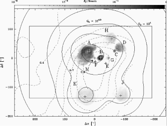
Figure 6: Overlay of UV field, [C ii] emission, and 6 cm radio continuum. Grey-scale: Image of the VLA 6 cm radio continuum (Tieftrunk et al. 1997). The box denotes the region observed with KOSMA. Solid contours: Contours of the calculated spatial structure of the FUV field smoothed to $75^{\prime\prime}$ resolution. The positions of the OB stars are marked with a $+$. Dashed contours: extended [C ii] emission observed by Howe et al. (1991) with the KAO at $80^{\prime\prime}$ resolution. Contour levels range from 40% to 90% in steps of 10% of the peak intensity of $314\,\mathrm{K}\,\mathrm{km}\,\mathrm{s}^{-1}$.

Table 5: H ii regions and exciting OB stars which were used to construct the two-dimensional FUV-field shown as drawn contours in Figure 6. The spectral type (col. (2)) is an average from the compilation of Tieftrunk et al. (1997). Total luminosities (col. (4)) assuming ZAMS stars are from Panagia (1973). Column (5) gives the corresponding names of infrared sources (Wynn-Williams et al. 1972; Richardson et al. 1989).

H ii	Spectral	Position	$L$	Remark
Region	Type	(${}^{\prime\prime},^{\prime\prime}$)	$10^{4}$L⊙
A	O5	$(25,21)$	$68.0$	IRS 2
B	O6.5	$(-20,1)$	$15.0$	IRS 3a
K	O6.5	$(32,-132)$	15.0
J	O8	$(-87,-129)$	6.5
D	O8.5	$(-76,34)$	$5.4$	IRS 10
Aa	O8.5	$(18,25)$	$5.4$	IRS 2a
H	O8.5	$(-58,67)$	$5.4$
F	O9.5	$(-3,-11)$	$3.8$	IRS 7
C	O9.5	$(-72,27)$	$3.8$	IRS 4
G	B0	$(-47,0)$	$2.5$
E	B0	$(-37,-18)$	$2.5$
Ma-g	B0	$(0,0)$	$7\times 2.5$	IRS 5
Ca	B1	$(-69,28)$	$0.5$	IRS 4
Sum			151.0

4.2 A map of [C ii] emission

Figure 6 shows the extended [C ii] ²P${}_{3/2}{-}^{2}$P_1/2 158 $\mu\mathrm{m}$ emission (Howe et al. 1991) in contours at a resolution of $80^{\prime\prime}$. The [C ii] emitting region shows a north-south extension and extends over all the H ii regions which have been identified in radio continuum emission studies (Tieftrunk et al. 1997). Interestingly, the north-south orientation is not seen in the atomic carbon maps nor in the CO maps (Figures 2). Neither is it seen in the FIR continuum at 158 $\mu$m observed by Howe et al. (1991) which shows a circular symmetry peaking at IRS 5. This could mean that [C ii] does not solely trace PDRs, i.e. the molecular cloud surfaces. A fraction of [C ii] emission may stem from the H ii regions and the diffuse outer halo. In the following paragraph, we estimate the contribution by the H ii regions in W3 Main.

In addition, the modelled FUV field does not trace well the observed distribution of [C ii]. The former shows a peak at IRS 5 while the latter shows a north-south orientated ridge of constant [C ii] emission. This mismatch is surprising since [C ii] is thought to be an accurate tracer of the FUV field. Howe et al. (1991) showed that a homogeneous cloud model cannot reconcile this particular discrepancy. Rather a clumpy cloud model has to be invoked with dense clumps immersed in a dilute interclump medium, allowing the FUV radiation to deeply penetrate into the cloud. Here, we try to improve on this analysis by using the new observations of [C i] and CO.

4.3 [C ii] emission from the ionized medium

[C ii] emission does partly stem from the H ii regions. However, the contribution of [C ii] emission from H ii regions to the observed [C ii] emission is in most cases found to be weak. We have calculated the fraction of [C ii] emission from the H ii regions in W3 Main using the emission measures and electron densities compiled by Tieftrunk et al. (1997) and the formalism of Russell et al. (1981) (cf. Crawford et al. 1985; Nikola et al. 2001). We found that the contribution is very low, varying between 0.1 and 0.7%.

This result appears to be valid also on much larger scales. Using the COBE Milky Way survey, Petuchowski & Bennett (1993) find that H ii regions contribute only $\sim 1\,$% of the total luminosity of the Galaxy in the [C ii] line.

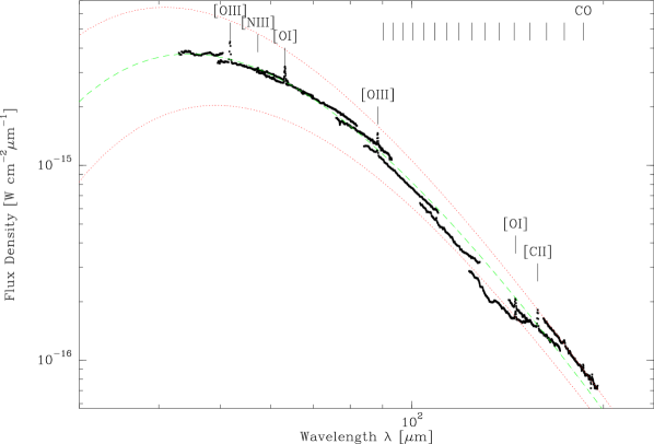
Figure 7: ISO/LWS spectrum of the IRS 5 position in W3 Main The overlapping LWS bands are clearly discernable. The dashed line is the isothermal grey body fit which results in $T_{\rm dust}=53$ K and $\beta=1.2$ for $A_{V}=40$ mag. For comparison, the drawn lines show the grey body for $58\,$K and $47\,$K dust temperature at the same $\beta$ value. The positions of several atomic fine structure and high-$J$ CO lines are marked.

Table 6: ISO/LWS integrated intensities of the FIR lines and the FIR continuum at IRS 5. Integrated intensities are listed in units of [$10^{-3}$erg s^-1 cm^-2 sr^-1] and were derived from the measured flux per beam using the beam sizes (col. (4)) and corrections for extended source emission given in Table 4.10 in the ISO-LWS Handbook v. 1.2. The listed errors only reflect the line fitting uncertainty. The intensity of the [O i]($145\,\mu$m) line is the average of two LWS detectors. The error is in this case the deviation from the individual fluxes.

IRS 5	$\lambda$	Integr.Intensity	HPBW
	[$\mu$m]		[′′]
CO 14–13	186.	0.21 $\pm$ 0.03	66.
CO 15–14	174.	0.30 $\pm$ 0.03	66.
CO 16–15	163.	0.08 $\pm$ 0.03	66.
CO 17–16	153.	0.13 $\pm$ 0.03	68.
[C ii]	158.	1.54 $\pm$ 0.03	68.
[O i]	145.	0.77 $\pm$ 0.13	68.
[N ii]	122.	0.06 $\pm$ 0.06	78.
[O iii]	88.	3.8 $\pm$ 0.2	76.
[O i]	63.	8.3 $\pm$ 0.3	86.
[N iii]	57.	1.7 $\pm$ 0.3	84.
[O iii]	52.	19 $\pm$ 1	84.
FIR-Continuum		13500

4.4 ISO/LWS data of IRS 5/W3 Main

We retrieved the FIR ISO/LWS data at IRS 5 from the data archive and reanalyzed it as described in Sect. 2.3.

4.4.1 Grey body fit

The far-infrared continuum at IRS 5 is modelled using the ISO/LWS data. We assumed an isothermal grey body spectrum $F_{\lambda}=\Omega B_{\lambda}(T_{\rm dust})(1-\exp^{-\tau_{\rm dust}})$, where the solid angle $\Omega$ was fixed to correspond to the average LWS HPBW of $\sim 75^{\prime\prime}$, $B_{\lambda}(T_{\rm dust})$ is the Planck function at temperature $T_{\rm dust}$, and the dust opacity is parametrized by $\tau_{\rm dust}=\tau_{V}(\lambda/\lambda_{V})^{-\beta}$. The total H₂ column density derived in Sect.3.6 corresponds to an optical extinction of $A_{V}=40$ mag$=1.086\,\tau_{V}$ (Bohlin et al. 1978) and was held fixed as well. A least squares fit of the dust temperature and the spectral index results in $T_{\rm dust}=53\pm 1$ K and $\beta=1.21\pm 0.02$ (Fig. 7). The total brightness, obtained by integrating over all wavelengths, is $2.1\,10^{-13}$ Wcm^-2beam^-1 or 13.5 erg s^-1 cm^-2 sr^-1. The total luminosity within the beam is $3.4\,10^{5}$ L_⊙. Comparison with Table 5 indicates that all of the FIR luminosity is powered by the O5 star associated with IRS 2 (Table 5).

Assuming $I_{\rm FIR}=2\times 1.6\,10^{-3}(4\pi)^{-1}G_{0}$  erg s^-1cm^-2sr^-1 (Kaufman et al. 1999), i.e. assuming that the stellar FUV flux is solely responsible for the FIR continuum, we estimate the FUV field at IRS 5 to be $G_{0}=5.3\,10^{4}$. This is only 13% of the FUV field estimated solely from the spectral types of the OB stars: $G_{0}=4\,10^{5}$ (Table 4) which may again indicate that a part of the stellar photons escape the cloud without heating the clouds. This issue will be discussed again in Chapter 4.5.4 when comparing with the results of the PDR modelling.

To improve on the analysis of the ISO/LWS continuum, a better calibration of the LWS bands would be needed and the variation of LWS beam sizes ($55^{\prime\prime}-90^{\prime\prime}$) would need to be taken into account.

Oldham et al. (1994) derive slightly higher values of $T_{\rm dust}=68$ K and $\beta=1.4$ from fitting a single-temperature grey body spectrum to FIR data at higher angular resolutions of $<27^{\prime\prime}$, indicating again an increase in temperature with smaller beam. They also fit an optical extinction of $A_{V}=281$ mag for a source diameter of $13^{\prime\prime}$. Comparing this $A_{V}$ with the $A_{V}$ we derive within a $75^{\prime\prime}$ beam, indicates a source size of $28^{\prime\prime}$.

4.4.2 Atomic fine structure lines

Integrated intensities of the transitions detected with ISO/LWS at IRS 5 are listed in Table 6.

Tracers of PDRs.

The lines of C ii, O i, and CO are prominent tracers of the PDRs at the surfaces of the molecular clouds. Of all FIR lines tracing the neutral medium, the $63\mu$m line of O i is the major coolant at IRS 5 being a factor of 4.1 stronger than the [C ii] line. Moreover, this [O i] transition may be optically thick and thus its intensity strongly reduced by foreground absorption. This is indirectly confirmed by detailed PDR modelling described in the Sect. 4.5.

The [C ii] integrated intensity detected with ISO/LWS is 70% of the intensity measured by Howe et al. (1991) with the KAO and thus in agreement within the expected calibration error.

Tracers of the ionized gas.

The ions N ii, O iii, N iii, have ionization potentials larger than 13.6 eV and their fine structure lines therefore trace the ionized medium. Although, the [N ii] line at $122\,\mu$m is not detected, the lower limit of the $[{C\textsc{ii}}]/[{N\textsc{ii}}]$ line flux ratio can be estimated to at least 27. A ratio of 9 (cf. Nikola et al. 2001) would be expected for [C ii] being emitted entirely from the ionized gas. This indicates that at most 33% of the [C ii] emission stems from the diffuse ionized medium. A more stringent estimate is derived using the properties of the H ii regions in W3 Main as discussed in Sect. 4.3.

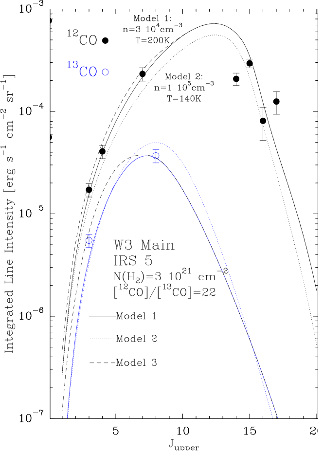
Figure 9: Integrated CO intensities as a function of upper rotational quantum number $J$ for IRS 5 in W3 Main and CO cooling curves produced by a non-LTE radiative transfer model. Rotational transitions upto $J=8$ were observed with KOSMA for which we plot the 15% uncertainty. The high-$J$ CO transitions upto $J=17$ were observed with ISO/LWS. We plot the uncertainties listed in Table 6. Model 3 is a two-component model adding the contributions of the warm gas (model 1) to a cold component at $T_{\rm kin}=40\,$K, $n=10^{3}$ cm^-3 containing 90% of the mass.

4.4.3 Carbon monoxide emission lines

Four high-lying rotational lines of gas phase CO were detected with ISO/LWS at IRS 5. These lines trace the hot and dense gas, upper level energies lie above 500 K and critical densities are about $10^{7}$ cm^-3 and higher. To better constrain the physical parameters, we used a non-LTE escape probability radiative transfer model (Stutzki & Winnewisser 1985) assuming a CO abundance of $8\,10^{-5}$ and using cross sections from Schinke et al. (1985). Figure 9 shows the CO and ¹³CO line integrated intensities observed with KOSMA and ISO/LWS.

Although the model simplifies the source structure by neglecting temperature and density gradients, and varying beam filling factors are not considered, common solutions can be found to fit all 9 observed line intensities. The minimum column density to reproduce the observed CO fluxes is $N$(H₂)$=3\,10^{21}$ cm^-2, only about 10% of the total H₂ column density at IRS 5 (Table 4). (We assumed line widths of 9 kms^-1 for the ¹²CO lines and 6 kms^-1 for the ¹³CO lines.) The column density is largely determined by the mid-$J$ CO transitions, rather independent of the kinetic temperatures and densities. The kinetic temperatures need to be high to reproduce the high-$J$ CO transitions detected with ISO/LWS while the ISO transitions are subthermally excited. However, two solutions exist which bracket the parameter space of acceptable models: 1. a high gas temperature of 200 K and rather low density of $3\,10^{4}$cm^-3 and 2. a lower gas temperature of 140 K and a higher gas density of $10^{5}$ cm^-3. Both solutions indicate a pressure ($n\,T$) of $(1-5)\,10^{7}$ Kcm^-3. The CO 15–14 transition is only slightly stronger than the CO 7–6 transition, the ratio of both intensities is 1.29. On the other hand, the intensity ratio of CO 15–14 over CO 1–0, derived from the model results, is about 500. Tieftrunk et al. (1998b) derived a kinetic temperature of 150 K at IRS 5 from ammonia observations, consistent with our results.

However, only about 10% of the gas is at these high temperatures and densities. A second phase must exist containing the bulk of the gas mass and at significantly lower temperatures. We model this phase assuming $N$(H₂)$=3\,10^{22}$ cm^-2, $T_{\rm kin}=40\,$K, $n=10^{3}$ cm^-3. The dashed curve in Figure 9 shows the combined flux (model 3) of the warm phase (model 1) and the cold phase. The cold phase hardly contributes to the observed cooling fluxes of the mid-$J$ and high-$J$ CO transitions, although it contains 90% of the gas mass.

A [CO]/[¹³CO] abundance ratio of 22 is needed to fit simultaneously the observed ¹³CO lines. The ¹³CO 8–7 line in particular is crucial in determining the column density and abundance ratio. The [CO]/[¹³CO] abundance is significantly lower than the ratio of 89 found by Mitchell et al. (1990) at sub-arcsecond resolutions, tracing the immediate hot and dense environment in front of IRS 5. The latter ratio is consistent with the canonical interstellar abundance of 65 (Langer & Penzias 1990). It is unlikely that ¹³CO fractionation plays a major role at W3/IRS 5 since the kinetic temperatures are much higher than 36 K, the energy gained in substituting ¹²C by ¹³C in CO. The low [CO]/[¹³CO] abundance ratio derived from the escape probability model may therefore indicate that a more detailed source model is needed, including density and kinetic temperature gradients along the line of sight. Indeed, in a more realistic model as the PDR model, the 15–14 and 4–3 CO lines are not produced by gas at the same temperature and the same density.

A similar analysis as we did for IRS 5 combining submillimeter and far-infrared CO lines was conducted by Harris et al. (1987); Stutzki et al. (1988), and Stacey et al. (1994) at FIR peaks of the Galactic star forming regions M 17, S 106, and in the Orion molecular cloud. The derived minimum column densities of the warm gas and the kinetic temperatures are very similar ($N$(CO)$=(0.5-6)\,10^{18}\,$cm^-2, $T_{\rm kin}=100-450$ K, $(1-4)\,10^{4}\,$cm^-3) to the solution we find in W3 IRS 5. These conditions appear to be typical for Galactic molecular clouds in the vicinity of massive star formation. Similar conditions of the warm molecular gas, but on a much larger scale of 180 pc are found in the starburst nucleus of NGC 253 by analyzing CO cooling curves (Bradford et al. 2004).

4.4.4 Line cooling from [C ii], [C i], CO, and [O i]

The ratio of [C ii] intensity over the FIR continuum within the ISO/LWS beam of $\sim 75^{\prime\prime}$ at IRS 5 is $1.1\,10^{-4}$ (cf. Table 6). The same ratio averaged over the entire mapped region is a factor 14 higher, i.e. $1.5\,10^{-3}$ (Howe et al. 1991). Similar values of about $10^{-4}$ as found locally at W3 IRS 5 have also been found in other Galactic star forming regions like Orion A, M 17, W 51, or DR 21 (see Table 5 in Stacey et al. 1991). On the other hand, the COBE large scale low resolution map of the Milky Way shows a higher and rather constant ratio with little scatter between $50\,10^{-4}$ and $170\,10^{-4}$ (Fixsen et al. 1999). [C ii]/FIR ratio ratios of upto 0.01 have been found in other Galactic clouds (Stacey et al. 1991) using KAO and in external galaxies (Stacey et al. 1991; Malhotra et al. 2001). Based on ISO observations, Malhotra et al. (2001) found typical [C ii]/FIR ratios for normal galaxies (excluding AGNs) in the range 0.01 to 0.001. However, there are again significant exceptions: two warm and active galaxies show ratios of less than $2\,10^{-4}$, reminicent of the ratio we find at IRS 5. A significant [C ii] deficiency has also been found in ULIRGs (Luhman et al. 1998). A number of explanations are discussed in the literature. One possibility is that increased $G_{0}/n$ ratios lead to increased positive grain charge which in turn leads to less efficient heating of the gas by photoelectrons from dust grains. See e.g. Kaufman et al. (1999) for a discussion.

The sum of all observed CO intensities is $1.0\,10^{-3}$erg s^-1cm^-2 sr^-1, only a fifth of the total modelled CO line cooling for $J$ upto 20 (Model 1). The total CO flux is only weakly influenced by self-absorption, since we have corrected for this effect to first order, and secondly, the CO cooling is mainly produced by the highly-excited lines which are less affected by self absorption. The importance of the unobserved transitions between $J=8$ and $J=13$ to the total cooling is evident from Figure 9 and from the escape probability analysis which shows that the peaks of the best fitting modelled cooling curves both lie near $J=12$.

The total CO cooling by far exceeds the gas cooling by the two carbon lines: $\Lambda_{\rm CO}/\Lambda_{\rm C}=123$. The two [O i] lines are more important: $\Lambda_{\rm O}/\Lambda_{\rm CO}=1.9$, $\Lambda_{\rm O}/\Lambda_{\rm CII}=6$. The relative contributions to the total gas cooling are $\Lambda_{\rm CO}=31.6\%$, $\Lambda_{\rm O}=58.7\%$, $\Lambda_{\rm CII}=9.7\%$, $\Lambda_{\rm C}=0.3\%$. The relative contribution of [O i] may be even stronger due to high optical depth and foreground absorption of the [O i]($63\,\mu$m) line. The total gas cooling flux is $15.5\,10^{-3}$erg s^-1cm^-2 sr^-1 and thus 0.1% of the dust cooling FIR flux.

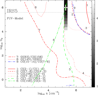
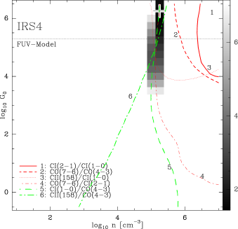
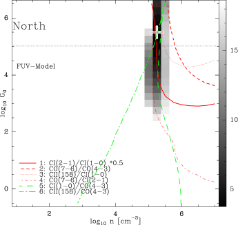
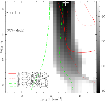
Figure 10: Results from the PDR model of Kaufman et al. (1999) at the four selected positions in W3 Main. Contours show the observed ratios of line integrated intensities as a function of FUV flux in units of the Habing field $G_{0}$ and the H₂ volume density $n$. We use the [C ii] data from KAO (Howe et al. 1991). The straight horizontal lines show the FUV field modelled from the embedded OB stars and smoothed to the resolution of the line data, i.e. $75^{\prime\prime}$ (Table 4). Greyscales denote the reduced $\chi^{2}$ derived from the observed line ratios, weighted with the uncertainty of 20%, and not taking into account the ratios of [O i](63$\,\mu$m) and CO 15–14 at IRS 5. The cross marks the best solution $\chi_{\rm min}^{2}$. Greyscales vary between 1 and 5 times $\chi_{\rm min}^{2}$.

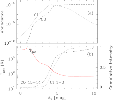
Figure 11: Variation of physical parameters with $A_{V}$ for a PDR model (Kaufman et al. 1999, Wolfire priv. comm.)with $n=1.8\,10^{5}$ cm^-3 and $G_{0}=10^{6}$ which is characteristic for IRS 5 (cf. Table 7). (a) Local abundances $n(X)/(n(H)+2n(H_{2}))$ of atomic carbon and CO. The CI abundance peaks at $A_{V}\sim 4.2\,$mag reaching $1.2\,10^{-4}$ while the CO abundance rises steadily with $A_{V}$ reaching an abundance of $1.4\,10^{-4}$ at $A_{V}=10\,$mag. (b) The gas temperature (drawn line) varies between 4000 K at the surface and $\sim 70$ K at $A_{V}=10$ mag. The contours labeled CO 15-14 and CI 1-0 show the line intensity integrated along $A_{V}$ from the outside in to greater depths and normalized to the integrated intensity at $A_{V}=10\,$mag. The CO 15-14 line stems from regions slightly further out and slightly warmer than the region where CI 1-0 is emitted. The extinction upto which half of the intensity is emitted, is 4.2 mag for CO 15-14 and 4.6 mag for CI 1-0. At these extinctions, the gas temperatures are 213 K and 140 K, respectively.

Table 7: Results of detailed PDR modelling at the four selected positions in W3 Main. The minimum $\chi^{2}$ was used to derive an estimate of the best fitting clump density $n_{\rm cl}$ and UV Flux. $T_{\rm surf}$ is the surface temperature of the corresponding clump predicted by the PDR model. The average density $n_{\rm av}$, the volume filling factor $\phi_{V}$, the average clump diameter $D_{\rm cl}$, and the number of clumps are derived using the PDR model results and the total beam averaged H₂ column density resulting from the above LTE analysis (Table 4). The area filling factor $\Phi_{A}$ is the ratio of observed [C ii] intensities over the modelled intensities.

$\Delta\alpha/\Delta\delta$	$\chi_{\rm min}^{2}$	$n_{\rm cl}$	UV Flux	$T_{\rm surf}$	$n_{\rm av}$	$\phi_{V}$	$D_{\rm cl}$	$N_{cl}$	$\phi_{A}$
$[^{\prime\prime},^{\prime\prime}]$		[$\log$(cm-3)]	[$\log(G_{0})$]	[K]	[cm-3]		[pc]
$0,0$ (IRS 5)	1.0	5.25	6	3970	$1.5\,10^{4}$	0.09	0.05	404	1.5
$-55.0,27.5$ (IRS 4)	1.4	5.25	6.25	4070	$1.6\,10^{4}$	0.09	0.07	188	1.2
$0,82.5$ (North)	3.7	5.25	5.5	3640	$5.8\,10^{3}$	0.03	0.03	467	0.8
$0,-82.5$ (South)	9.2	5.00	6.5	3480	$7.3\,10^{3}$	0.07	0.05	340	1.2

4.5 Detailed PDR modelling of the submillimeter and far-infrared emission

We have used the results of PDR models of Kaufman et al. (1999) to compare with the observed line ratios. These models assume a constant density of a semi-infinite plane-parallel slab illuminated by the interstellar radiation field and improve on the older models of Tielens & Hollenbach (1985). PAHs are found to dominate the grain-photoelectric heating and are therefore included. ¹³C is not included in the chemical network. The model computes a simultaneous solution for the chemistry, radiative transfer, and the thermal balance in PDRs.

4.5.1 Estimating density and FUV field from the line ratios

We have compared the models with selected line flux ratios of the PDR tracers: CO (4–3, 7–6), [C i] (1–0, 2–1), [C ii] 158$\mu$m, and, at IRS 5, [O i](63$\mu$m, 145$\mu$m) and CO (15–14). Figure 10 shows the detailed comparison at the four selected positions in W3 Main (cf. Fig. 4, Tables 2, 3, 4, 6). The plots span a density range from $n=10$ to $10^{7}$ cm^-3 and a FUV flux range from $G_{0}=0.3$ to $3\,10^{6}$, i.e. the full range of the Kaufman models. Horizontal dashed lines mark the beam averaged FUV flux estimated above in Sect. 4.1 from the spectral types of the OB stars.

We do not expect to find one solution of $G_{0},n$ for each observed position, i.e. an intersection of contours at one point. This is because, first, the observational calibration error of 20% of the ratios and, second, the line emission surely cannot be entirely described by slabs of only one density. The analysis given here will however allow to derive average clump densities, average impinging FUV fields, and several other average clump parameters. Indeed, the line ratio contours shown in Figure 10 for the four representative positions do not all intersect. However, the observed four ratios of [C ii]/[C i] 1–0, CO 7–6/[C i] 2–1, [C i] 1–0/CO 4–3, and [C ii]/CO 4–3 do almost intersect at $n_{\rm cl}=2\,10^{5}$ cm^-3 and $G_{0}>10^{5}$ at the three positions IRS 5, IRS 4, and North. The ratios of CO over [C i] lines largely determine the densities and are rather independent of $G_{0}$. The high FUV fields are largely determined by the [C ii] over [C i] ratios and also by the [C ii] over CO 4–3 ratios. We find still higher densities of upto $10^{7}$ cm^-3 from the two ratios of [C i] 2–1/1–0 and CO 7–6/4–3 at all positions.

At IRS 5, we also obtained the CO 15–14/7–6 ratio. Very similar to the CO 7–6/4–3 ratio, it indicates high densities of $\sim 6\,10^{5}$ cm^-3 for $G_{0}>10^{5}$. However, these ratios are still consistent with the best fitting solutions within a deviation of better than 50%. Figure 11 shows the variation of abundances, temperatures, and intensities with optical extinction for the best fitting PDR model at IRS 5: $n=1.8\,10^{5}$ cm^-3, $G_{0}=10^{6}$, i.e. $G_{0}/n=5.5$ cm³ (cf. Table 7). It shows that the bulk of CO 15–14 emission stems from a region of $\sim 210\,$K temperature while the bulk of CI 1–0 emission stems from a region of $\sim 140$ K. While the detailed PDR modelling shows a strong temperature gradient, the characteristic CO temperature of 210 K is only slightly higher than the results of the single component escape-probability modelling of the mid and high-$J$ CO lines described in sec. 4.4.3 (Fig. 9). There, we had fitted temperatures and densities of between 140 K at $10^{5}$ cm^-3 and 200 K at $3\,10^{4}$ cm^-3. However, a homogeneous model with 200 K at $n=10^{5}$ cm^-3 would be predicting stronger CO lines than considered in Section 4.4.3. Thus, with regard to CO emission, the esc. prob. model and the PDR model do not agree with each other completely.

The LTE analysis of the CI line ratio in section 3.4.2 indicated CI excitation temperatures of $>120\,$K at IRS 5, in rough agreement with the detailled PDR modelling.

4.5.2 The [O i]($63\,\mu$m) line is optically thick

From ISO/LWS at IRS 5, we also obtained ratios of [O i](63 $\mu$m)/[C ii] and [O i](145 $\mu$m)/(63 $\mu$m). Assuming a FUV field of at least $G_{0}=10^{5}$, these ratios indicate low densities of less than $10^{4}$ cm^-3, clearly deviating from the above scenario. However, the [O i]($63\,\mu$m) line is optically thick all over the parameter space (Kaufman et al. 1999) and thus probably strongly affected by self-absorption of the cold foreground gas component also visible in the low-$J$ and mid-$J$ CO lines. The line strengths of the CO 4–3 and 3–2 lines are reduced by a factor of 1.5 because of self-absorption (Fig. 5). Decreasing the [O i](145 $\mu$m)/(63 $\mu$m) ratio by a factor of 2 would lead to a contour intersecting with the best fitting $G_{0},n$ solution of the other ratios. However, the [O i](63 $\mu$m)/[C ii] would need to be increased by a factor of 15. Thus, the [O i](63 $\mu$m) line is not consistently described in the current model. Velocity resolved observations to study the structure of FIR line shapes and thus confirm self-absorbed profiles will become possible with GREAT/SOFIA (Güsten et al. 2003) in the near future.

4.5.3 The quality of the fits

To quantify the correspondance of the ratios, we have plotted in Figure 10 the $\chi^{2}$ per degree of freedom, i.e. the reduced $\chi^{2}$, of the observed ratios in greyscales. To allow for a comparison between the four positions, we did not take into account here the ratios of [O i] and CO 15–14 which were only obtained at IRS 5. For the six remaining ratios, the degree of freedom is $5-2$. The best fitting solution $\chi_{\rm min}^{2}$ is marked by a cross and listed in Table 7. A value of $\chi_{\rm min}^{2}$ near 1 is found at IRS 5 and IRS 4 which signifies that the ratios agree well within their observational errors. The agreement is worse at the two other positions.

The best fitting FUV fluxes of the PDR models are surprisingly high, i.e. upto $G_{0}=2\,10^{6}$, though with a higher uncertainty compared to the best fitting densities. At all positions, the fitted FUV flux is higher than the beam averaged, purely geometrically attenuated FUV fluxes estimated above from the luminosity of the embedded OB stars.

4.5.4 Line and FIR cooling at IRS 5 revisited

The line fluxes observed with KOSMA and ISO/LWS at IRS 5 had already been discussed in Chapter 4.4.4. Here, these fluxes are compared with the absolute fluxes predicted by the best fitting PDR model at IRS 5 (cf. Table 7). Table 8 shows that model and observations are in agreement to within 50% for the total fluxes of CO, [C ii], and [C i]. The [C ii] flux observed with the KAO listed here is a factor of 1.5 larger than the flux observed with ISO which equals the PDR model result.

As discussed in Sec. 4.5.2, the [O i] $63\,\mu$m line is predicted to be much stronger than observed. The total observed [O i] cooling is only 10% of the modelled flux.

As already noted above, the FUV flux derived by fitting the line ratios to the PDR model is $G_{0}=10^{6}$, surprisingly high relative to the beam averaged FUV flux derived from the OB stars, $G_{0}=4\,10^{5}$, and higher than the FUV flux derived from the beam averaged FIR field, $G_{0}=5\,10^{4}$ (Sec. 4.4.1). Correspondingly, the FIR flux derived from the modelled $G_{0}$ via $I_{\rm FIR}=2\times 1.6\,10^{-3}(4\pi)^{-1}G_{0}$ erg s^-1cm^-2sr^-1 (Kaufman et al. 1999), is high, $I_{\rm FIR}=260$  erg s^-1 cm^-2 sr^-1, i.e. a factor $20$ higher than the observed flux.

This indicates that the line emission is mainly excited in the dense inner regions near the embedded OB stars where the FUV flux is higher. The FIR continuum on the other hand also stems from the colder outer surroundings thus leading to a lower average FIR intensity.

Table 8: Observed fluxes at IRS 5 in units of $10^{-3}$ erg s^-1 cm^-2 sr^-1 compared to the best fitting PDR model with $n=1.8\,10^{5}$ cm^-3, $G_{0}=10^{6}$. The total gas cooling is $\Lambda_{\rm gas}=\Lambda_{\rm CII}+\Lambda_{\rm CI}+\Lambda_{\rm CO}+\Lambda_{\rm OI}$. ^a The total “observed” CO cooling $\Lambda_{\rm CO}$ was derived from the esc. prob. model fitted to the observed fluxes (cf. Chapter 4.4.4).

	$\Lambda_{\rm CII}$	$\Lambda_{\rm CI}$	$\Lambda_{\rm CO}$	$\Lambda_{\rm OI}$	$\Lambda_{\rm gas}$	$\Lambda_{\rm FIR}$
Observed	2.2	0.04	4.9a	9.1	15.5	13500
PDR-Model	1.5	0.03	7.3	93.7	103.0	260000
Ratio	1.5	1.3	0.7	0.1	0.15	0.05

4.5.5 A clumpy PDR model

Using these results in combination with the total beam averaged H₂ column density resulting from the LTE analysis at the four positions (Table 4), allows to derive more physical parameters characterizing the line emitting gas. We assume here, that line emission arises in individual clumps immersed in an interclump medium which is not emitting in the observed transitions. Motivated by the morphology of the KOSMA maps shown in Figure 2, we assume conservatively that the line of sight extent of the cloud is $D_{\rm cloud}=0.84$ pc ($75^{\prime\prime}$). This allows to use the total column density to derive a rough estimate of the average volume density $n_{av}$ per beam. The ratio of $n_{av}$ with the average clump density $n_{cl}$ derived above, gives the volume filling factor of the clumps $\Phi_{V}$. The area filling factor $\Phi_{A}$ of the clumps can be estimated from the ratio of observed intensities $I_{\rm obs}$ over the modelled intensities $I_{\rm mod}$ - it can be larger than unity for optically thin emission. The clump diameter $D_{\rm cl}$ can be estimated from $D_{\rm cloud}\,\Phi_{V}/\Phi_{A}$. The number of clumps is then given by $\Phi_{V}(D_{\rm cloud}/D_{\rm cl})^{3}$.

Table 7 summarizes the resulting quantities at the four positions. Results are much less certain for the southern position than for IRS 5. Only less than 10% of the volume is filled with a few hundred clumps per beam area. Clumps have a typical diameter of 0.05 pc, i.e. $4.4^{\prime\prime}$, and are thus unresolved. The resulting typical clump mass is $M=n_{\rm cl}\,4/3\,\pi\,(D_{\rm cl}/2)^{3}=0.44\,$M_⊙.

The area filling factor derived from [C ii] is $\sim 1\pm 0.5$. Area filling factors and clump diameters are not significantly changed when e.g. using the modelled [C i] 1–0 intensities instead. Another reason for discrepancies between the modelled and the observed intensities are geometrical effects. Kaufman et al. (1999) assume a face-on geometry, a viewing angle of $<90^{\circ}$ would lead to an increase in the intensity of optically thin lines.

We cannot exclude the possibility that a fraction of the CI and CII emission stems from the interclump medium since the CI and CII transitions have critical densities of only $5\,10^{2}$ to $3\,10^{3}$ cm^-3 (cf. Kaufman et al. 1999).

These results confirm the results of Howe et al. (1991) which had been based solely on the [C ii] map and on the estimated FUV field. They had found that a cloud clumpy model can be adjusted to be roughly consistent with the observed [C ii] morphology. Their best fitting model is very similar to ours: their clumps have a density of $n_{\rm cl}\sim 10^{5}\,$cm^-3, the volume filling factor is $\Phi_{V}\sim 0.05-0.07$.

Further indirect support for our clumpy source model comes from the analysis of CS 2–1, 5–4, and 7–6 FCRAO and KOSMA small maps of W3 Main by Ossenkopf et al. (2001). The observed line profiles are best fitted by an average density of $0.7\,10^{4}$ cm^-3 within a radius of 1 pc while the minimum central density reaches $5\,10^{6}$ cm^-3, higher than the clump density we have derived from the PDR analysis, but similar to the high densities inferred from the [C i] 2–1/1–0 and CO 7–6/4–3 ratios.

Direct evidence for the existence of very dense and small molecular clumps is delivered by VLA maps of Ammonia in W3 Main at $3^{\prime\prime}$ resolution by Tieftrunk et al. (1998a). These show several clumps of $\sim 0.02$ pc radius and densities of a few $10^{7}$ cm^-3 in the vicinity of IRS 5 and IRS 4.

Still higher densities at temperatures of almost 600 K are known to exist on scales of less than $0.01$ pc ($<2000$ AU, $<1^{\prime\prime}$) in the immediate vicinity of IRS 5 from the absorption study of Mitchell et al. (1990).

Our scenario of many small, high density clumps with a small volume, but a high area filling factor should nevertheless not be taken too literal. It simply implies that the cloud structure is very far off a homogeneous cloud, but shows a very much broken up structure with high density contrasts and steep density gradients within the cloud.

5 Summary

1. We have mapped the W3 Main region in the two fine structure lines of atomic carbon and in several mid-$J$ CO transitions using KOSMA. All maps show a peak of integrated intensities near IRS 5 and IRS 4 with a steady drop of intensities in all directions. Spectral line maps show structure down to the spatial resolution limit of $>42^{\prime\prime}$, i.e. $>0.5\,$pc. To obtain a common spatial resolution, all data discussed below are at a common resolution of $75^{\prime\prime}$ (0.84 pc). In addition, we have obtained ISO/LWS data at IRS 5.

2. We find a constant CO 7–6/4–3 line integrated intensity ratio of $\sim 1$ at all positions in W3 Main after correcting for self-absorption seen in the ¹²CO lines in the vicinity IRS 5. Assuming thermalized emission, this ratio indicates excitation temperatures in excess of 85 K and densities in excess of $\sim 10^{6}\,$cm^-3 for the gas emitting these mid-$J$ CO lines. A more detailed non-LTE analysis however reveals that densities of $\sim 10^{5}$ cm^-3 are sufficient to explain the observed CO cooling fluxes.

3. The observed high [C i] 2–1/1–0 line ratios of between 1.3 and 2.9 indicate optically thin carbon emission and excitation temperatures of about 100 K.

4. LTE analysis of carbon column densities show that the C i/CO abundance ratios stays constant at $\sim 0.11$. The fractional abundances of C ii/C i/CO are $\sim 20:10:70$ at IRS 5, rising to $\sim 32:7:61$ in the south of W3 Main.

5. A model of the FUV field distribution, derived from the embedded OB stars, assuming pure geometrical attenuation, ignoring the cloud density structure, and smoothed to $75^{\prime\prime}$ resolution, shows a peak field at IRS 5 of $G_{0}=10^{5.5}$ dropping to values below $10^{3.5}$ in the outskirts of W3 Main.

6. The north-south orienation of the [C ii] emission (Howe et al. 1991) is not seen in the maps of [C i] and CO emission. Nor is it seen in the modelled FUV field distribution.

7. At IRS 5, the (average) dust temperature of the FIR emission detected by ISO/LWS is 53 K with a spectral index of $\beta=1.2$. The [O i] 63 $\mu$m line is a factor 4 stronger than the [C ii] 158$\,\mu$m line. The [C ii]/FIR flux ratio is 0.01%. We estimate that less than 1% of the [C ii] emission stems from the H ii regions in W3 Main. The relative contributions to the total gas cooling are $\Lambda_{\rm CO}=31.6\%$, $\Lambda_{\rm O}=58.7\%$, $\Lambda_{\rm CII}=9.7\%$, $\Lambda_{\rm C}=0.3\%$. $\Lambda_{\rm CO}$ refers to the total CO cooling modelled with the escape probability radiative transfer model in Sec. 4.4.4. All other numbers refer to the observed values. The ratio of $\Lambda_{\rm gas}/\Lambda_{\rm dust}$ is 0.1%.

8. We have used the PDR model of Kaufman et al. (1999) to estimate the average densities of the emitting region and the impinging FUV fields from the observed line ratios at four selected positions. The [O i](63$\mu$m) line is probably optically thick and strongly affected by self-absorption in the colder foreground material at IRS 5, and thus discarded from the further analysis. The remaining six line ratios indicate a common solution of $G_{0}\sim 10^{6}$ and $n_{\rm cl}\sim 2\,10^{5}$ cm^-3 at all four positions. The reduced $\chi^{2}$ is low at IRS 5, IRS 4, and the northern position, but much higher at the Southern position where no well defined common solution is found. We have assumed that all line emission arises in individual clumps immersed in an interclump medium which is not emitting in the observed transitions. We find that the emitting gas consists of a few hundred clumps per 0.84 pc beam, filling between 3 and 9% of the volume, with a typical clump radius of 0.025 pc ($2.2^{\prime\prime}$), and typical mass of 0.44 M_⊙.

9. The line ratios of [C i] 2–1/1–0 and CO 7–6/4–3 are consistent with very high clump densities of upto $10^{7}$ cm^-3 in the framework of the PDR model. This finding may be explained by a more detailed model of clumps having a variation of densities (and masses). A more detailed model of W3 Main would also need to take into account absorption by foreground gas.

Although the discussed model scenario is not able to reproduce each detail of the line intensities and their variation within the cloud, it is remarkable that the scenario of a UV penetrated clumpy cloud is able to reproduce the relative (and to a large degree also the absolute) intensities of some dozen lines simultaneously with only a relatively small set of model parameters such as the clump average density and size, most other parameters being constrained by the UV intensity distribution and the temperature and chemical gradients calculated through the PDR models.