Characterizing Inflationary Perturbations: The Uniform Approximation

Abstract

The spectrum of primordial fluctuations from inflation can be obtained using a mathematically controlled, and systematically extendable, uniform approximation. Closed-form expressions for power spectra and spectral indices may be found without making explicit slow-roll assumptions. Here we provide details of our previous calculations, extend the results beyond leading order in the approximation, and derive general error bounds for power spectra and spectral indices. Already at next-to-leading order, the errors in calculating the power spectrum are less than a per cent. This meets the accuracy requirement for interpreting next-generation CMB observations.

I Introduction

Recent observations of the cosmic microwave background (CMB) cmbobs ; rev and of the galaxy distribution in real and redshift space lssobs have dramatically improved our knowledge of the large-scale Universe. Results from these observations have been largely consistent with the inflationary paradigm of cosmology, since it appears that the Universe is at critical density and that the observed structure in the Universe arose from the gravitational collapse of adiabatic, Gaussian, and nearly-scale-invariant primordial density fluctuations, a key prediction of simple inflation models.

The idea that an inflationary expansion, aside from solving cosmological puzzles such as the horizon and flatness problems, also provides a natural mechanism for the generation of primordial fluctuations was realized around the time the model was first proposed infpertorig . Early estimates already established the essential adiabatic, Gaussian, and nearly-scale invariant nature of the perturbation spectrum. However, these estimates were rather crude and their true value lay in providing very significant qualitative guidance rather than accurate quantitative information. As the prospect of testing inflation and even distinguishing between individual models from precision CMB observations became more realistic, attention was increasingly focused on improving the understanding and predictive control of the theory underlying the generation of fluctuations. The development of the gauge invariant treatment of cosmological perturbations givb ; givs ; ivrevs1 ; ivrevs2 and its application to inflation ivrevs2 ; givinf ; givvfm ; givdhl was of great help in clarifying and systematizing the calculations involved.

The simple nature of the perturbation spectrum characteristic of inflation arose from models where inflation was caused by the dynamics of a single scalar field in a relatively featureless potential, evolving in an effectively friction-dominated ‘slow-roll’ regime LLKCBA ; slowrev . It was realized that in more complex inflation models (multiple fields, nontrivial potentials) it is possible to engineer the spectra in a variety of ways including violation of scale-invariance and introduction of isocurvature fluctuations. However, data from present-day observations do not demand the consideration of dynamically exotic inflation models.

Inflation predicts a spectrum of metric perturbations in the scalar (density) and tensor (gravitational wave) sectors, the vector component being naturally suppressed. Both scalar and tensor perturbations cause anisotropy in the CMB temperature anisotropy . Scalar fluctuations seed formation of large-scale structure in the Universe, while the tensor perturbations lead to a stochastic gravitational wave background gravbg . In addition, tensor modes cause a potentially observable polarization of the CMB, a target for next-generation CMB observations polar . Given the variety, precision, and volume of data now and soon to be available from the various probes of primordial fluctuations, it is important to provide controlled theoretical analyses for various classes of inflation models.

One obvious application of such an analysis lies in comparing theoretical predictions to observations in order to test specific inflation models. In addition, there is the prospect of obtaining information about the slow-roll potential via a controlled inverse analysis of observational data, the so-called ‘reconstruction’ program recon (for a review see LLKCBA ). Finally, there is also the more general question of whether the inflationary paradigm itself can be tested from observations. Regarding this question, recent activity has focused on identifying classes of inflation models distinguished by their differing observational signatures HT rather than trying to reconstruct a specific inflationary potential. A recent discussion of parameter estimation using input from inflation calculations can be found in Ref. paraminf .

To expand further on the above, we note that while inflation is the most compelling cosmological paradigm, it is not without its competitors other . None of the alternative scenarios, including structure formation via topological defects (definitively ruled out by observations), or string-inspired models such as the ekpyrotic and cyclic Universe scenarios, as yet may be viewed as offering convincing competition. Nevertheless, an important question arises in the comparison of predictions particular to generic models of inflation to predictions one might expect on purely general grounds or from other models. A good example of this is provided by the spectral index $n_{S}$ characterizing the scalar perturbation spectrum. The Harrison-Zeldovich choice $n_{S}=1$ hz is aesthetically natural, independent of inflation. A high-precision observational detection of $n_{S}$ provides a good target for inflation models if $n_{S}$ is indeed slightly different from unity. (Clearly, an intuitive argument such as that of Harrison and Zeldovich cannot be refined further without a corresponding theoretical framework.) Related to this, another important point is that inflation predictions for the scalar and tensor spectra are not mutually independent. Future measurements of the CMB can provide tests of this dependency, thus it is important to state precisely the appropriate ‘consistency relations’ cons and the accuracy to which they can be calculated for a range of inflation models.

The equations governing the evolution of the scalar and tensor perturbations can be solved numerically. For specific models, it can scarcely be argued that an approximate analytical result is competitive with a mode-by-mode numerical solution of the equations. Nevertheless analytic results can be extremely powerful in providing generic results valid for many classes of models. Accurate analytic results also greatly reduce the computational requirements for the reconstruction program. Therefore some effort has concentrated on improving theoretical predictions by sharpening the slow-roll analysis. In this regard, approximations based on certain slow-roll assumptions have been criticized on multiple fronts. It has been argued that error control is not adequate and that they are not systematically improvable wms ; ms . There have been some efforts to alleviate this situation srimprov ; schwarzetal , however, they are based on restrictive assumptions (e.g., $n_{S}\simeq 1$) and often lead to complicated mathematical formulations.

Recently, we presented an analysis of the inflationary perturbation spectrum for single-field models based on applying a uniform approximation to the relevant mode equations hhjm . This analysis goes beyond the slow-roll approximation, does not make restrictive assumptions, has definite error bounds, and is systematically improvable. In this paper we implement the method beyond leading order and provide general error bounds on power spectra and spectral indices. While our general expressions for the spectral indices are nonlocal, we can derive local expressions for $n_{S}$ and $n_{T}$ by employing a further approximation. We also demonstrate that by Taylor-expansion of our local results, expressions of the slow-roll type can easily be obtained. Finally, in order to demonstrate the accuracy of the uniform approximation explicitly, we discuss its application to an exactly solvable inflation model.

The organization of the paper is as follows: Section II provides the essential background to understanding the problem of computing the power spectrum, Section III explains the uniform approximation, Section IV gives the leading order results, Section V provides the results at next order, and Section VI contains the results of Section IV simplified to a local form. Here we also encapsulate the conventional slow-roll results and derive the analogous results from the uniform approximation. Section VII considers a special example which possesses an exact solution and uses this to demonstrate the characteristic features of the uniform approximation. In Section VIII we comment briefly on Bessel function approximants. Section IX concludes with a discussion of the results obtained and an outline of future work. Appendix A provides a short list of the relevant definitions and equations for linearized perturbations in an FRW universe. Appendix B contains the technical details behind the error formulae of the uniform approximation.

II Background

The cosmic microwave background and the large-scale distribution of matter both provide information on the primordial perturbation spectrum, albeit ‘processed’ by physics during the radiation and matter-dominated phases. Extraction of information from large scale structure observations is complicated by the nonlinear effects of the gravitational instability and various sources of observational bias. Fortunately, the physics of the photon distribution is very different from that of the mass distribution: As a consequence of radiation pressure, the CMB is very uniform and fluctuations in it can be treated adequately by a linearized analysis.

The generation of perturbations during inflation is due to the amplification of quantum vacuum fluctuations by the dynamics of the background spacetime. Of course, the post-inflationary epoch must also be understood in order to make a connection with observations. A serious treatment of the dynamics of the post-inflationary phase is necessarily quite complicated as various effects such as reheating, particle decay, etc. have to be taken into account. Fortunately, it turns out that an accurate accounting of much of this physics is not required in order to make inflation predictions for CMB anisotropies and the large-scale distribution of matter.

The modern treatment of fluctuations generated by inflation is in turn based on the gauge-invariant treatment of linearized fluctuations in the metric and field quantities (Appendix A) givb ; givs ; ivrevs1 ; ivrevs2 ). A particularly convenient quantity for characterizing the perturbations is the intrinsic curvature perturbation of the comoving hypersurfaces givdhl , $\zeta\equiv u/z$, where $u\equiv a(\delta\phi+\phi^{\prime}A/h)$ and $z\equiv a\phi^{\prime}/h$, with $a$, the scale factor, the prime denoting a derivative with respect to conformal time, $h\equiv a^{\prime}/a$, $\delta\phi$ the perturbation in the homogeneous background scalar field, $\phi$, and $A$, a quantity characterizing a perturbation of the background metric (details are given in Appendix A). As shown in Appendix A, the gauge-invariant quantity, $u$, satisfies the dynamical equation

$$u^{\prime\prime}-\Delta u-{z^{\prime\prime}\over z}u=0.$$ (1)

It follows immediately that $\zeta$ is approximately constant in the long wavelength limit $k\rightarrow 0$. This is true during the inflationary phase as well as in the post-reheating era. Moreover, the Einstein equations can be used to connect the gravitational potential $\Phi_{A}$ and $\zeta$ so that a computation of the power spectrum of $\zeta$ provides all the information needed (aside from the transfer functions) to extract the temperature anisotropy of the CMB. Details of this procedure can be found in Refs. ivrevs2 ; ms ; ms2 . We will return to some aspects of this analysis below.

The calculation of the relevant power spectra involves a computation of the two-point functions for the appropriate quantum operators, e.g.,

$$\langle 0|\hat{u}(\eta,{\bf x})\hat{u}(\eta,{\bf x}+{\bf r})|0\rangle=\int_{0}^{\infty}{dk\over k}{\sin kr\over kr}P_{u}(\eta,k),$$ (2)

the operator $\hat{u}$ being written as

$$\hat{u}(x)=\int{d^{3}k\over(2\pi)^{3/2}}\left[\hat{a}_{k}u_{k}(\eta)\hbox{e}^{i{\bf k}\cdot{\bf x}}+\hat{a}_{k}^{\dagger}u_{k}^{*}(\eta)\hbox{e}^{-i{\bf k}\cdot{\bf x}}\right],$$ (3)

where $\hat{a}_{k},~{}\hat{a}_{k}^{\dagger}$ are annihilation and creation operators, respectively, such that $[\hat{a}_{k},\hat{a}_{k^{\prime}}^{\dagger}]=\delta_{kk^{\prime}}$, and defining the vacuum state $\hat{a}_{k}|0\rangle=0$ $\forall k$. The complex amplitude $u_{k}(\eta)$ satisfies

$$u_{k}^{\prime\prime}+\left(k^{2}-{z^{\prime\prime}\over z}\right)u_{k}=0.$$ (4)

Solving Eqn. (4) is the fundamental problem in determining the primordial power spectrum $P_{u}$ (or $P_{\zeta}$). The corresponding mode equation for tensor perturbations is given by

$$v_{k}^{\prime\prime}+\left(k^{2}-{a^{\prime\prime}\over a}\right)v_{k}=0.$$ (5)

Equations (4) and (5) have the mathematical form of Schrödinger equations. A simple approach to analytical approximation of Eqns. (4) and (5) relies on the fact that exact solutions exist in the limits $k^{2}\gg\left|z^{\prime\prime}/z\right|$, $\left|a^{\prime\prime}/a\right|$ (short wavelength) and $k^{2}\ll\left|z^{\prime\prime}/z\right|$, $\left|a^{\prime\prime}/a\right|$ (long wavelength) or, as will be made more explicit below, as $-k\eta\rightarrow\infty$ and $k\eta\rightarrow 0^{-}$. For scalar perturbations,

$$u_{k} \rightarrow {1\over\sqrt{2k}}e^{-ik\eta}~{}~{}\left(k^{2}\gg\left|z^{\prime\prime}/z\right|,~{}-k\eta\rightarrow\infty\right),$$ (6)

$$u_{k} \rightarrow A_{k}z~{}~{}\left(k^{2}\ll\left|z^{\prime\prime}/z\right|\right).$$ (7)

Here, the short wavelength solution corresponds to the choice of an adiabatic vacuum for modes on length scales much smaller than the scale set by the curvature. The long wavelength solutions correspond to the growing mode on scales much larger than the Hubble length. (Analogous solutions exist for gravitational wave perturbations.)

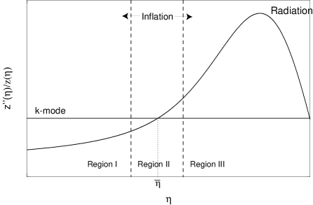
Figure 1: Sketch of the potential barrier for density perturbations. The vertical dashed lines delineate the three different regions where the solution for $u_{k}$ is investigated as explained in the text. $\bar{\eta}$ marks the point where the $k$-mode enters into the potential barrier, the turning point. Inflation lasts over a wide $\eta$-range, extending Region II as indicated by the arrows. In the far right of Region III radiation dominates.

The long wavelength solution for $\zeta_{k}=u_{k}/z$ is just the ($k$-dependent) constant $A_{k}$ of Eqn. (7). In order to determine the corresponding power spectrum $P_{\zeta}(k)\equiv P_{S}(k)$, the main task is to fix the unknown constant $A_{k}$ by connecting the two asymptotic solutions. We sketch the situation in Fig. 1. The large-$k$ regime lies in region I and the small-$k$ regime lies in region III. The two asymptotic solutions may be connected either by a matching procedure performed in region II, typical of the slow-roll class of approximations discussed further below, or, as performed here, by constructing a global interpolating solution. Once $A_{k}$ is determined, the power spectrum for $\zeta$ can be computed in the regime ($k\rightarrow 0$) of actual interest,

$$P_{S}(k)={k^{3}\over 2\pi^{2}}\left|A_{k}\right|^{2},$$ (8)

where the index $S$ indicates scalar perturbations.

III The Uniform Approximation

We begin our discussion of the uniform approximation by making the substitution

$${z^{\prime\prime}\over z}\equiv{1\over\eta^{2}}{\cal{C}}^{2}(\eta)$$ (9)

in Eqn. (4), yielding

$$u_{k}^{\prime\prime}(\eta)+\left[k^{2}-\frac{{\cal{C}}^{2}(\eta)}{\eta^{2}}\right]u_{k}(\eta)=0.$$ (10)

A similar substitution can be made for the case of tensor perturbations.

If, in Eqn. (10), we make the assumption that ${\cal{C}}$ is constant, (which is the case for power law inflation, see Section VII) then an exact solution in terms of Bessel functions is immediate. The problem is to solve the equation when ${\cal{C}}$ is not constant but is a slowly varying function of time. Our aim is to do this without being forced to state ${\cal{C}}(\eta)$ in any real detail. The method we will use is the technique of uniform approximation as presented by Olver Olver . We now provide a brief summary of this treatment for the differential equation of interest (10).

The differential equation we wish to solve is of the general form

$${d^{2}u\over d\eta^{2}}=\left[b^{2}g(\eta)+q(\eta)\right]u.$$ (11)

Depending on the behavior of $b^{2}g(\eta)+q(\eta)$ this equation has different approximating solutions. In the case that $g(\bar{\eta})=0$ at the point $\bar{\eta}$, so $\bar{\eta}$ is a turning point, the solution is expressed in terms of Airy functions; if $g(\eta)$ has a pole of order $n\geq 2$ the Liouville-Green (LG) approximation must be employed Olver . The Liouville-Green approximation is essentially equivalent to the familiar Wentzel-Kramers-Brillouin (WKB) approximation; for an application of WKB to computing perturbations from inflation, see Ref. ms03 . In our case the relevant function is $-k^{2}+{\cal{C}}^{2}(\eta)/\eta^{2}$; we have a turning point which will depend on the explicit form of $g(\eta)$ and a pole of order $2$ in the limit $\eta\rightarrow 0^{-}$. Therefore, we have an Airy solution around the turning point which goes over to an LG solution for conformal time approaching zero. As will be shown later, this approximation fits the exact behavior of the solution accurately. For the two approximating solutions (Airy and LG), the convergence criteria are established in the following way. Assume that we have a pole of order $n\geq 2$ at a finite endpoint $a_{2}$ and that $g(\eta)$ and $q(\eta)$ are meromorphic functions of the form

$$g(\eta) = {1\over(a_{2}-\eta)^{2}}\sum_{s=0}^{\infty}f_{s}(a_{2}-\eta)^{s},$$

$$q(\eta) = {1\over(a_{2}-\eta)^{2}}\sum_{s=0}^{\infty}g_{s}(a_{2}-\eta)^{s}.$$ (12)

Then the error control function (see Appendix B) converges if $g_{0}=-1/4$. For a detailed proof of this fact, see Ref. Olver . For the error control criteria to be satisfied in our case, we must make the choices

$$g(\eta) = {1\over\eta^{2}}\left[{\cal{C}}^{2}(\eta)+{1\over 4}\right]-k^{2},$$ (13)

$$\equiv {\nu_{S}^{2}(\eta)\over\eta^{2}}-k^{2},$$

$$q(\eta) = -{1\over 4\eta^{2}}.$$ (14)

The final form of Eqn. (4) then becomes

$$u_{k}^{\prime\prime}=\left\{-k^{2}+{1\over\eta^{2}}\left[\nu_{S}^{2}(\eta)-{1\over 4}\right]\right\}u_{k},$$ (15)

where $\nu_{S}^{2}=(z^{\prime\prime}/z)\eta^{2}+1/4$ and the turning point is at $k^{2}=\nu_{S}^{2}({\bar{\eta}}_{S})/{\bar{\eta}}_{S}^{2}$. Note that the turning point, ${\bar{\eta}}_{S}$, is a given function of $k$.

In an exactly analogous fashion, the equation for the tensor modes (5) is written in the form

$$v_{k}^{\prime\prime}=\left\{-k^{2}+{1\over\eta^{2}}\left[\nu_{T}^{2}(\eta)-{1\over 4}\right]\right\}v_{k},$$ (16)

where $\nu_{T}^{2}=(a^{\prime\prime}/a)\eta^{2}+1/4$ and the turning point is at $k^{2}=\nu_{T}^{2}({\bar{\eta}}_{T})/{{\bar{\eta}}_{T}}^{2}$.

Unlike the approach of matching solutions through regions I, II, and III, the idea of a uniform approximation is to provide a single approximating solution which converges uniformly in all three regions with a global, finite error bound. The normalization is determined once and for all by simply matching to the exact solution as $k\rightarrow\infty$.

To continue, we follow Olver in defining a new independent variable $\xi$ and a new dependent variable $U$, given by Olver

$$\xi\left({d\xi\over d\eta}\right)^{2}=g(\eta),~{}~{}u=\left({d\xi\over d\eta}\right)^{-1/2}U.$$ (17)

In terms of the new variables, Eqn. (11) becomes

$${d^{2}U\over d^{2}\xi}=\left[b^{2}\xi+\psi(\xi)\right]U,$$ (18)

where

$$\psi(\xi) = \left[4g(\eta)g^{\prime\prime}(\eta)-5g^{\prime 2}(\eta)\right]\frac{\xi}{16g^{3}(\eta)}$$ (19)

$$+\frac{\xi q(\eta)}{g(\eta)}+\frac{5}{16\xi^{2}},$$

$$\frac{2}{3}\xi^{3/2} = -\int_{\eta}^{\bar{\eta}}\sqrt{g(\eta)}d\eta,~{}~{}~{}\eta\geq\bar{\eta}$$ (20)

$$\frac{2}{3}\left(-\xi\right)^{3/2} = \int_{\eta}^{\bar{\eta}}\sqrt{-g(\eta)}d\eta,~{}~{}~{}\eta\leq\bar{\eta}.$$ (21)

Now imagine neglecting $\psi(\xi)$ as a first approximation; then the solution to the differential equation is given immediately in terms of Airy functions. In the next order where $\psi(\xi)$ is no longer neglected, the derivation of the solution $u$ becomes more involved. Fortunately, in Ref. Olver the general solution for Eqn. (11) in the uniform approximation to all orders is derived with error bounds to be

$$u_{2n+1}^{(1)}(b,\xi) = \left[\frac{g(\eta)}{\xi}\right]^{-1/4}\left[{\rm Ai}(b^{2/3}\xi)\sum_{s=0}^{n}\frac{A_{s}(\xi)}{b^{2s}}\right.$$

$$\left.+\frac{{\rm Ai}^{\prime}(b^{2/3}\xi)}{b^{4/3}}\sum_{s=0}^{n-1}\frac{B_{s}(\xi)}{b^{2s}}+\epsilon_{2n+1}^{(1)}\right],$$

$$u_{2n+1}^{(2)}(b,\xi) = \left[\frac{g(\eta)}{\xi}\right]^{-1/4}\left[{\rm Bi}(b^{2/3}\xi)\sum_{s=0}^{n}\frac{A_{s}(\xi)}{b^{2s}}\right.$$

$$\left.+\frac{{\rm Bi}^{\prime}(b^{2/3}\xi)}{b^{4/3}}\sum_{s=0}^{n-1}\frac{B_{s}(\xi)}{b^{2s}}+\epsilon_{2n+1}^{(2)}\right],$$

with coefficients defined by an iterative procedure,

$$A_{0}(\xi) = 1~{}~{}~{}~{}{\rm w.l.o.g.},$$ (24)

$$B_{s}(\xi) = \frac{\pm 1}{2\sqrt{\pm\xi}}\int_{0}^{\xi}\left[\psi(v)A_{s}(v)-A_{s}^{\prime\prime}(v)\right]\frac{dv}{\sqrt{\pm v}},$$ (25)

$$A_{s+1}(\xi) = -\frac{1}{2}B^{\prime}_{s}(\xi)+\frac{1}{2}\int\psi(\xi)B_{s}(\xi)d\xi,$$ (26)

where the upper signs are to be taken on the right of the turning point $\bar{\eta}$ and the lower signs on the left of the turning point. The error terms $\epsilon_{2n+1}^{(1)}$ and $\epsilon_{2n+1}^{(2)}$ are discussed in Appendix B. In the next and following Sections, we will calculate the leading and next-to-leading order solution for Eqn. (15) with explicit error bounds and derive the corresponding power spectra and spectral indices.

IV Results at Leading Order

We now turn to the specific form of the approximating solutions at leading order. Taking $n=0$ in Eqns. (III) and (III) we find a solution for $u_{k}(\eta)$ containing a part valid to the left of the turning point ($\eta\leq\bar{\eta}$) and a part valid to the right of the turning point ($\eta\geq\bar{\eta}$). The unnormalized solutions are

$$u^{(1)}_{k,\scriptscriptstyle\lessgtr}(\eta) = u^{(1)}_{k,1,\scriptscriptstyle\lessgtr}(\eta)\left[1+\epsilon_{k,1,\scriptscriptstyle\lessgtr}^{(1)}(\eta)\right],$$ (27)

$$u^{(2)}_{k,\scriptscriptstyle\lessgtr}(\eta) = u^{(2)}_{k,1,\scriptscriptstyle\lessgtr}(\eta)\left[1+\epsilon_{k,1,\scriptscriptstyle\lessgtr}^{(2)}(\eta)\right],$$ (28)

with

$$u^{(1)}_{k,1,{\scriptscriptstyle\lessgtr}}(\eta) = \left[f_{\scriptscriptstyle{\lessgtr}}(k,\eta)/g_{S}(k,\eta)\right]^{1/4}{\rm Ai}[f_{\scriptscriptstyle\lessgtr}(k,\eta)],$$

$$u^{(2)}_{k,1,\scriptscriptstyle\lessgtr}(\eta) = \left[f_{\scriptscriptstyle\lessgtr}(k,\eta)/g_{S}(k,\eta)\right]^{1/4}{\rm Bi}[f_{\scriptscriptstyle\lessgtr}(k,\eta)],$$ (29)

$$f_{\scriptscriptstyle\lessgtr}(k,\eta) = \mp\left\{\pm\frac{3}{2}\int_{\eta}^{\bar{\eta}_{S}}d\eta^{\prime}\left[\mp g_{S}(k,\eta^{\prime})\right]^{1/2}\right\}^{2/3},$$ (30)

$$g_{S}(k,\eta) = \frac{\nu_{S}^{2}(\eta)}{\eta^{2}}-k^{2},$$ (31)

$$|\epsilon_{k,1,\scriptscriptstyle\lessgtr}^{(1)}(\eta)| \leq \frac{1}{\lambda}\frac{M(f_{\scriptscriptstyle\lessgtr})}{E(f_{\scriptscriptstyle\lessgtr}){\rm Ai}(f_{\scriptscriptstyle\lessgtr})}\left\{e^{\lambda{\cal V}_{\eta,\alpha}({\cal E})}-1\right\},$$ (32)

$$|\epsilon_{k,1,\scriptscriptstyle\lessgtr}^{(2)}(\eta)| \leq \frac{1}{\lambda}\frac{E(f_{\scriptscriptstyle\lessgtr})M(f_{\scriptscriptstyle\lessgtr})}{{\rm Bi}(f_{\scriptscriptstyle\lessgtr})}\left\{e^{\lambda{\cal V}_{\beta,\eta}({\cal E})}-1\right\},$$ (33)

where the lower index $1$ reflects the order of the approximation, the functions with index $<$ are taken on the left of the turning point, and those with the index $>$ are to be taken on the right of the turning point. $M(\eta)$, $N(\eta)$, ${\cal V}_{\alpha,\beta}$, and $\lambda$ are defined in Appendix B, and the error control function ${\cal E}(\eta)$ is given by

$${\cal E}(\eta) = -{1\over 4}\int d\eta\left\{g_{S}^{-3/2}\left[g_{S}^{\prime\prime}-{5\over 4}\frac{(g_{S}^{\prime})^{2}}{g_{S}}-{g_{S}\over\eta^{2}}\right]\right\}$$ (34)

$$\pm{5\over 24|f_{\scriptscriptstyle\lessgtr}|^{3/2}}.$$

Inserting the explicit expression for $g_{S}(k,\eta)$, Eqn. (31), and integrating by parts leads to

$${\cal E}(\eta) = \frac{\nu_{S}(\nu_{S}^{\prime}\eta-\nu_{S})}{(\nu_{S}^{2}-k^{2}\eta^{2})^{3/2}}\pm{5\over 24|f_{\scriptscriptstyle\lessgtr}|^{3/2}}$$

$$+\int\frac{d\eta}{4\eta\sqrt{\nu_{S}^{2}-k^{2}\eta^{2}}}\left\{1-\left[\frac{\nu_{S}(\nu_{S}^{\prime}\eta-\nu_{S})}{\nu_{S}^{2}-k^{2}\eta^{2}}\right]^{2}\right\}.$$

The errors terms $\epsilon_{k,1,\scriptscriptstyle\lessgtr}^{(1,2)}(\eta)$ in Eqns. (27) and (28) encapsulate the contributions to $u_{k,1,\scriptscriptstyle\lessgtr}^{(1,2)}(\eta)$ beyond leading order. The general solution for $u_{k}(\eta)$ is a linear combination of the two fundamental solutions $u_{k}^{(1)}(\eta)$ and $u_{k}^{(2)}(\eta)$, viz.,

$$u_{k}(\eta)=Au_{k}^{(1)}(\eta)+Bu_{k}^{(2)}(\eta),$$ (36)

independent of the order of the approximation. In order to fix the constants $A$ and $B$ we have to construct a linear combination of $u^{(1)}_{k}(\eta)$ and $u^{(2)}_{k}(\eta)$ such that the result has the form $u_{k}(\eta)=e^{-ik\eta}/\sqrt{2k}$ in the limit $k\rightarrow\infty$. In this limit, the domain of interest is region I, far to the left of the turning point. In this case, for well-behaved $\nu_{S}$, $f_{<}(k,\eta)$ is large and negative and we can employ the asymptotic forms

$${\rm Ai}(-x) = \frac{1}{\pi^{1/2}x^{1/4}}\cos\left(\frac{2}{3}x^{3/2}\right)-\frac{\pi}{4},$$

$${\rm Bi}(-x) = -\frac{1}{\pi^{1/2}x^{1/4}}\sin\left(\frac{2}{3}x^{3/2}\right)-\frac{\pi}{4}.$$ (37)

Making the choices,

$$A=\sqrt{\frac{\pi}{2}}e^{i\frac{\pi}{4}},~{}~{}B=-i\sqrt{\frac{\pi}{2}}e^{i\frac{\pi}{4}},$$ (38)

we find

$$u_{k,1,<}(\eta)=\lim_{-k\eta\rightarrow\infty}{C\over\sqrt{2k}}~{}\exp\left\{i\frac{3}{2}\left[f_{<}(k,\eta)\right]^{3/2}\right\},$$ (39)

which is the required adiabatic form of the solution at short wavelengths and as $\eta\rightarrow-\infty$ fulling . $C$ is a constant phase factor which is irrelevant when computing the power spectrum.

The $\eta\rightarrow 0^{-}$ limit defines the region of interest for calculating power spectra and the associated spectral indices. In this region, the $1/\eta^{2}$ pole dominates the behavior of the solutions and the Airy solution goes over to the LG solution. The LG form of the solution is more tractable than the Airy form, leading to simple expressions for the spectral indices. We now demonstrate how the Airy solution for small $\eta$ approaches the LG solution. The linear combination of Eqns. (27) and (28) in first order with the appropriate normalization is given by

$$u_{k,1,\scriptscriptstyle\lessgtr}(\eta)=\sqrt{\frac{\pi}{2}}Cf_{\scriptscriptstyle\lessgtr}^{1/4}(k,\eta)g_{S}^{-1/4}(k,\eta)\left[{\rm Ai}(f_{\scriptscriptstyle\lessgtr})-i{\rm Bi}(f_{\scriptscriptstyle\lessgtr})\right],$$ (40)

with the error bound

$$|\epsilon_{k,1,\scriptscriptstyle\lessgtr}(\eta)| \leq \frac{\sqrt{2}}{\lambda}\left\{\right.\left[\exp(\lambda{\cal V}_{\eta,\alpha}({\cal E}))-1\right]$$

$$+\left.\left[\exp(\lambda{\cal V}_{\beta,\eta}({\cal E}))-1\right]\right\}$$

derived from Eqns. (32), (33), (139), and (141). (The explicit form of the variation of ${\cal E}$ will be discussed below.) For small $\eta$ we are on the right of the turning point; the argument of the Airy functions, i.e., $f_{>}(k,\eta)$, becomes large and the Airy functions can be approximated by

$${\rm Ai}(x) = \frac{1}{2\sqrt{\pi}}~{}x^{-1/4}\exp\left(-\frac{2}{3}x^{2/3}\right),$$ (41)

$${\rm Bi}(x) = \frac{1}{\sqrt{\pi}}~{}x^{-1/4}\exp\left(\frac{2}{3}x^{2/3}\right),$$ (42)

which leads to

$$u_{k,1,>}(\eta) = {C\over\sqrt{2}}g_{S}^{-1/4}(k,\eta)\left[{\frac{1}{2}}\exp\left\{-\frac{2}{3}\left[f_{>}(k,\eta)\right]^{3/2}\right\}\right.$$ (43)

$$\left.-i\exp\left\{\frac{2}{3}\left[f_{>}(k,\eta)\right]^{3/2}\right\}\right].$$

For computing the power spectra in the $k\eta\rightarrow 0^{-}$ limit, only the growing part of the solution is relevant:

$$u_{k,1,>}(\eta)=\lim_{k\eta\rightarrow 0^{-}}-iC\sqrt{{-\eta\over 2\nu_{S}(\eta)}}\exp\left\{\frac{2}{3}\left[f_{>}(k,\eta)\right]^{3/2}\right\}.$$ (44)

Once the approximate solutions to Eqns. (4) and (5) have been found in the manner described above, the relevant power spectra can easily be computed. The definition of the scalar power spectrum for $\zeta$, where it is understood that all time-dependent quantities are to be evaluated in the limit $\eta\rightarrow 0^{-}$, is

$$P_{S}(k) = \lim_{k\eta\rightarrow 0^{-}}\frac{k^{3}}{2\pi^{2}}\left|\frac{u_{k}(\eta)}{z(\eta)}\right|^{2}$$ (45)

$$= \lim_{k\eta\rightarrow 0^{-}}\frac{k^{3}}{2\pi^{2}}\left|\frac{u_{k,1,>}(\eta)}{z(\eta)}\right|\left|1+\epsilon_{k,1,>}(\eta)\right|^{2}$$

$$= \lim_{k\eta\rightarrow 0^{-}}P_{1,S}(k)\left[1+\epsilon_{k,1,S}^{P}(\eta)\right],$$

with

$$\epsilon_{k,1,S}^{P}=2\epsilon_{k,1,>},$$ (46)

$P_{1,S}(k)$ denoting the power spectrum for the scalar perturbations in the leading order approximation and dropping a second-order term in $\epsilon_{k,1,>}$. Substituting the LG expression for $u_{k}$ from Eqn. (44), we have

$$P_{1,S}(k)=\lim_{k\eta\rightarrow 0^{-}}\frac{k^{3}}{4\pi^{2}}\frac{1}{|z(\eta)|^{2}}\frac{-\eta}{\nu_{S}(\eta)}\exp\left\{\frac{4}{3}\left[f_{>}(k,\eta)\right]^{3/2}\right\},$$ (47)

with the error bound for the power spectrum given in Eqn. (46).

We now discuss the variation of $\mathcal{E}$. (See Appendix B for a short discussion on the variation of a function in general.) We are interested in the error bound of $u_{k,1}$ over the full domain of interest $-\infty<\eta<0^{-}$, which implies $\beta=-\infty$ and $\eta\rightarrow 0^{-}$. In the general case,

$${\cal V}_{-\infty,\eta}({\cal E})=\sum|{\cal E}(\alpha)-{\cal E}(\beta)|,$$ (48)

where the sum is over all individual monotonic subintervals $(\alpha,\beta)\subseteq(-\infty,\eta)$ of ${\cal E}$. In the special case of monotonic ${\cal E}$ over the full range of $\eta$ the answer can be given in a simplified form: By inserting the definition of $g_{S}(k,\eta)$ from Eqn. (31) into Eqn. (34) and integrating by parts we find for the variation of the error control function:

$${\cal V}_{-\infty,\eta}({\cal E}) = \left|-\frac{1}{2\nu_{S}}-\frac{1}{4}\int\frac{d\eta}{\eta\sqrt{\nu_{S}^{2}-k^{2}\eta^{2}}}\right.$$ (49)

$$\hskip 5.69046pt\left.\times\left\{1-\left[\frac{\nu_{S}(\nu_{S}^{\prime}\eta-\nu_{S})}{\nu_{S}^{2}-k^{2}\eta^{2}}\right]^{2}\right\}\right|,$$

where it is understood that $\eta$ has to be taken in the limit $\eta\rightarrow 0^{-}$. With this expression the error bound for the power spectrum given in Eqn. (46) is completely determined.

The calculation for the tensor power spectrum follows along the same lines, yielding

$$P_{1,T}(k)=\lim_{k\eta\rightarrow 0^{-}}\frac{k^{3}}{4\pi^{2}}\frac{1}{|a(\eta)|^{2}}\frac{-\eta}{\nu_{T}(\eta)}\exp\left\{\frac{4}{3}\left[\tilde{f}_{>}(k,\eta)\right]^{3/2}\right\},$$ (50)

with the error being controlled exactly in the same manner as in Eqns. (46) and (49) with the subscripts $S\rightarrow T$ and $\tilde{f}(k,\eta)$ indicating that $g_{S}(k,\eta)$ in Eqn. (29) has to be replaced by $g_{T}(k,\eta)$.

Before proceeding to the computation of the spectral indices, we make a few observations on the nature of the error term above. In previous work hhjm we have shown that the error term in the case of constant $\nu$ introduces a $k$-independent amplitude correction for the power spectrum which does not affect the spectral index; therefore the uniform approximation for the spectral index is exact in that case. In a later section we explicitly discuss this calculation. It turns out to be possible to utilize this result in a general way, and we turn to this now.

Suppose that we split the effective potential into two terms, writing

$$\nu^{2}(\eta)-\frac{1}{4}=\nu^{2}(0)-\frac{1}{4}+\nu^{2}(\eta)-\nu^{2}(0).$$ (51)

Further we define a corresponding splitting of the error term, $\epsilon_{k,1,>}=\epsilon_{0}+\tilde{\epsilon}$, where $\epsilon_{0}$ is the error term for the case of constant $\nu(\eta)$, the constant being given by $\nu(0)$. Following Olver, the total error term and the error term $\epsilon_{0}$ each satisfies an integral equation Olver ; using these we easily derive an integral equation for $\tilde{\epsilon}$ with a somewhat different inhomogeneity. By construction, this inhomogeneity is reduced in size compared to the inhomogeneity which appears in the integral equation for the full error term $\epsilon$. Using the fact that the error term for constant $\nu(\eta)$ is $k$-independent, in this way we demonstrate that the full error term can be written as a sum of two terms: $\epsilon_{0}$ which is $k$-independent and $\tilde{\epsilon}$ which has the property that it vanishes identically for constant $\nu(\eta)$ and satisfies an integral equation with a reduced inhomogeneity. Explicit calculation, applying the theorem of Olver in the slightly generalized context, gives a relative error bound of the form

$$\left|{\tilde{\epsilon}(\eta)}\right|\leq\frac{1}{\mathrm{Bi}(f_{\scriptscriptstyle\lessgtr})}E(f_{\scriptscriptstyle\lessgtr})M(f_{\scriptscriptstyle\lessgtr})\Phi(f_{\scriptscriptstyle\lessgtr})\exp[\lambda\mathcal{V}_{\alpha,\eta}(\mathcal{E})],$$ (52)

where $E(f_{\scriptscriptstyle\lessgtr})$ and $M(f_{\scriptscriptstyle\lessgtr})$ are the comparison functions introduced in the appendix and used in the discussion above, and where $\Phi(f_{\scriptscriptstyle\lessgtr})=\mathcal{V}_{\alpha,\eta}(\mathcal{E}-\mathcal{E}_{0})$; here $\mathcal{E}$ is the full error control function and $\mathcal{E}_{0}$ is the error control function for the constant $\nu(\eta)$ approximant.

This splitting therefore resums the error contributions which arise purely from the constant part of $\nu(\eta)$ and separates them into an explicit $k$-independent additive contribution to the full error, leaving a term which is quantitatively smaller and vanishes in the case of constant $\nu(\eta)$. This shows why we expect the uniform approximation to the spectral index to be a much better approximation than a direct application of the Olver theory would indicate.

Next we discuss the evaluation of the spectral indices. The generalized spectral index for scalar perturbations can be obtained from the power spectrum via

$$n_{S}(k)=1+\frac{d\ln P_{S}}{d\ln k}.$$ (53)

Differentiation of the power spectrum with respect to $k$ is straightforward. It is important to note that the turning point $\bar{\eta}_{S}$ is a function of $k$, since $k=-\nu_{S}(\bar{\eta}_{S})/|\bar{\eta}_{S}|$ where $\nu_{S}(\bar{\eta}_{S})$ is the value of $\nu_{S}(\eta)$ at the turning point $\eta=\bar{\eta}_{S}$. Using this relation, one finds

$$n_{1,S}(k)=4-2k^{2}\lim_{k\eta\rightarrow 0^{-}}\int_{\bar{\eta}_{S}}^{\eta}\frac{d\eta^{\prime}}{\sqrt{g_{S}(k,\eta^{\prime})}}.$$ (54)

Following from the discussion above, the error in the spectral index arises only from the $k$-dependent part of the error in the power spectrum, which vanishes in the case of constant $\nu_{S}$. Thus the error in the spectral index is sensitive only to the time variation of $\nu_{S}$. To estimate this error, the spectral index as written in Eqn. (53) can be expressed via the leading order power spectrum in the following form:

$$n_{S}(k) = 1+\frac{d\ln(P_{1,S}+\epsilon_{k,1,S}^{P})}{d\ln k}$$ (55)

$$= 1+\frac{d\ln P_{1,S}}{d\ln k}+k\frac{d\epsilon_{k,1,S}^{P}}{dk}$$

$$\equiv n_{1,S}(k)+\epsilon_{k,1,S}^{n},$$

with

$$\epsilon_{k,1,S}^{n}={k}\frac{d\epsilon_{k,1,S}^{P}}{dk}$$ (56)

Here we have neglected error terms of order $\epsilon^{2}$. We can estimate $|\epsilon_{k,1,S}^{n}|$ by using the next-order contribution to the power spectrum (Section V), leading to the final result

$$\epsilon_{k,1,S}^{n}(\eta) \approx -\frac{k^{2}}{\sqrt{2}}\int\frac{\eta d\eta}{(\nu_{S}^{2}-k^{2}\eta^{2})^{3/2}}$$

$$\times\left[1-5\nu_{S}^{2}\left(\frac{\nu_{S}-\nu_{S}^{\prime}\eta}{\nu_{S}^{2}-k^{2}\eta^{2}}\right)^{2}\right].$$

Again, it is understood that $\eta$ has to be taken in the limit $\eta\rightarrow 0^{-}$, thus the spectral index defined in Eqn. (54) has no time-dependence.

The above analysis can be carried out for tensor perturbations in an identical fashion, including the error estimation, with the replacement $\nu_{S}\rightarrow\nu_{T}$. The spectral index for gravitational waves is given by

$$n_{1,T}(k)=3-2k^{2}\lim_{k\eta\rightarrow 0^{-}}\int_{\bar{\eta}_{T}}^{\eta}\frac{d\eta^{\prime}}{\sqrt{g_{T}(k,\eta^{\prime})}}.$$ (58)

Approximate evaluation of the integrals in Eqns. (54) and (58) can be performed to yield more familiar forms for the spectral indices as shown in Section VI.

V Next-to-Leading Order

To proceed to the next order, we first write the unnormalized solution for $u_{k}$, following directly from Eqns. (III) and (III):

$$u^{(1)}_{k,3\scriptscriptstyle\lessgtr}(\eta) = \left[f_{\scriptscriptstyle\lessgtr}(k,\eta)/g_{S}(k,\eta)\right]^{1/4}\left\{{\rm Ai}[f_{\scriptscriptstyle\lessgtr}(k,\eta)]\left(A_{0}[f_{\scriptscriptstyle\lessgtr}(k,\eta)]\right.\right.$$ (59)

$$+\left.\left.A_{1}[f_{\scriptscriptstyle\lessgtr}(k,\eta)]\right)+{\rm Ai}^{\prime}[f_{\scriptscriptstyle\lessgtr}(k,\eta)]B_{0}[f_{\scriptscriptstyle\lessgtr}(k,\eta)]\right\},$$

$$u^{(2)}_{k,3\scriptscriptstyle\lessgtr}(\eta) = \left[f_{\scriptscriptstyle\lessgtr}^{1/4}(k,\eta)/g_{S}(k,\eta)\right]^{1/4}\left\{{\rm Bi}[f_{\scriptscriptstyle\lessgtr}(k,\eta)]\left(A_{0}[f_{\scriptscriptstyle\lessgtr}(k,\eta)]\right.\right.$$ (60)

$$+\left.\left.A_{1}[f_{\scriptscriptstyle\lessgtr}(k,\eta)]\right)+{\rm Bi}^{\prime}[f_{\scriptscriptstyle\lessgtr}(k,\eta)]B_{0}[f_{\scriptscriptstyle\lessgtr}(k,\eta)]\right\},$$

with

$$A_{0}[f_{\scriptscriptstyle\lessgtr}(k,\eta)] = 1,$$ (61)

$$B_{0}[f_{\scriptscriptstyle\lessgtr}(k,\eta)] = \frac{\pm 1}{2\sqrt{\pm f_{\scriptscriptstyle\lessgtr}(k,\eta)}}\int_{0}^{f_{\scriptscriptstyle\lessgtr}}\frac{\psi(v)}{\sqrt{\pm v}}dv,$$ (62)

$$A_{1}[f_{\scriptscriptstyle\lessgtr}(k,\eta)] = -\frac{1}{2}B_{0}^{\prime}[f_{\scriptscriptstyle\lessgtr}(k,\eta)]$$ (64)

$$+\frac{1}{2}\int\psi[f_{\scriptscriptstyle\lessgtr}]B_{0}[f_{\scriptscriptstyle\lessgtr}(k,\eta)]d[f_{\scriptscriptstyle\lessgtr}(k,\eta)].$$

The error bounds in next-to-leading order are given by [derived from Eqns. (137) and (B)]:

$$|\epsilon_{k,3,\scriptscriptstyle\lessgtr}^{(1)}| \leq 2E^{-1}(f_{\scriptscriptstyle\lessgtr})M(f_{\scriptscriptstyle\lessgtr}){\cal W}_{f_{\scriptscriptstyle\lessgtr},\beta},$$ (65)

$$|\epsilon_{k,3,\scriptscriptstyle\lessgtr}^{(2)}| \leq 2E(f_{\scriptscriptstyle\lessgtr})M(f_{\scriptscriptstyle\lessgtr}){\cal W}_{\alpha,f_{\scriptscriptstyle\lessgtr}},$$ (66)

with

$${\cal W}_{f_{\scriptscriptstyle\lessgtr},\beta} = \exp\left\{2\lambda\mathcal{V}_{f_{\scriptscriptstyle\lessgtr},\beta}(|f_{\scriptscriptstyle\lessgtr}|^{1/2}B_{0})\right\}\mathcal{V}_{f_{\scriptscriptstyle\lessgtr},\beta}(|f_{\scriptscriptstyle\lessgtr}|^{1/2}B_{1}),$$

$${\cal W}_{\alpha,f_{\scriptscriptstyle\lessgtr}} = \exp\left\{2\lambda\mathcal{V}_{\alpha,f_{\scriptscriptstyle\lessgtr}}(|f_{\scriptscriptstyle\lessgtr}|^{1/2}B_{0})\right\}\mathcal{V}_{\alpha,f_{\scriptscriptstyle\lessgtr}}(|f_{\scriptscriptstyle\lessgtr}|^{1/2}B_{1}),$$

and

$$B_{1}(f_{\scriptscriptstyle\lessgtr}) = \frac{\pm 1}{2\sqrt{\pm f_{\scriptscriptstyle\lessgtr}}}\int_{0}^{f_{\scriptscriptstyle\lessgtr}}\frac{dv}{\sqrt{\pm v}}[\psi(v)A_{1}(v)-A^{\prime\prime}_{1}(v)],$$

$$A^{\prime\prime}_{1}(v) = -\frac{1}{2}B_{0}^{\prime\prime\prime}(v)+\frac{1}{2}[\psi^{\prime}(v)B_{0}(v)+\psi(v)B^{\prime}_{0}(v)],$$

recursively derived from Eqns. (25) and (26).

As in leading order, the general solution $u_{k}(\eta)$ is a linear combination of $u_{k}^{(1)}(\eta)$ and $u_{k}^{(2)}(\eta)$. Fortunately, we will not have to calculate the normalization again; in the limit $\eta\rightarrow-\infty$ the Bunch-Davies vacuum is the exact solution of the differential equation for $u_{k}(\eta)$, and, in this limit, all corrections from the next-to-leading order terms are subdominant and of no interest.

A further simplification follows from the fact that only the growing solution, $u_{k}^{(2)}$, is relevant to determining the power spectrum and spectral index and that we can restrict ourselves to the solution for $u_{k}$ in the limit $k\eta\rightarrow 0^{-}$. Employing once again the approximation for the Bi-function for large, positive argument, Eqn. (42), and in addition, the approximation for its derivative,

$${\rm Bi}^{\prime}(x)=\frac{1}{\sqrt{\pi}}~{}x^{1/4}\exp\left(\frac{2}{3}x^{2/3}\right),$$ (71)

the normalized $u_{k}(\eta)$ in the relevant regime is

$$u_{k,3,>}(\eta) \stackrel{{\scriptstyle k\eta\rightarrow 0^{-}}}{{=}} -iC\sqrt{-{\eta\over\pi\nu_{S}(\eta)}}\exp\left\{\frac{2}{3}\left[f_{>}(k,\eta)\right]^{3/2}\right\}$$ (72)

$$\times\left\{1-\frac{1}{2}B^{\prime}_{0}(f_{>})+\sqrt{f_{{>}}(k,\eta)}B_{0}(f_{>})\right.$$

$$\left.+\frac{1}{2}\int\psi(f_{>})B_{0}(f_{>})d(f_{>})\right\},$$

where the error bound is given by

$$|\epsilon_{k,3,>}|\leq 2f_{>}^{-1/4}\exp{\left\{\frac{2}{3}\left[f_{>}(k,\eta)\right]^{3/2}\right\}}{\cal W}_{\alpha,f_{\scriptscriptstyle\lessgtr}}.$$ (73)

Analyzing $B_{0}$ in detail shows that the derivative $B_{0}^{\prime}$ and the integral over $\psi B_{0}$ are subdominant in the limit $k\eta\rightarrow 0^{-}$. Hence the only term leading to a correction of the power spectrum is $B_{0}$ itself. From the general expression (45), the power spectrum at next-to-leading order is

$$P_{2,S}(k)\stackrel{{\scriptstyle k\eta\rightarrow 0^{-}}}{{=}}P_{1,S}(k)|1+2\sqrt{f_{>}(k,\eta)}B_{0}[f_{{>}}(k,\eta)]|,$$ (74)

with $P_{1,S}(k)$ as defined in Eqn. (47) and

$$B_{0}(f_{>}) = \frac{1}{2\sqrt{f_{>}}}\int_{0}^{f_{>}}\frac{\psi(v)}{\sqrt{v}}dv,$$ (75)

$$\psi(v) = \frac{5}{16v^{2}}+\frac{v\left(4g_{S}g^{\prime\prime}_{S}-5g_{S}^{\prime 2}\right)}{16g^{3}_{S}}-\frac{v}{4\eta^{2}g_{S}}.$$ (76)

The first term in $B_{0}$ [after writing out $\psi(v)$ according to Eqn. (76)] can be integrated immediately. The contribution from the lower integration limit, which appears divergent at a first glance, cancels with contributions from the other terms in the integral. This can be shown by expanding $\psi(v)$ around zero and integrating explicitly. The error bound can be calculated in the same way as in leading order. We find

$$P_{S}(k)=\lim_{k\eta\rightarrow 0^{-}}\frac{k^{3}}{2\pi^{2}}\left|\frac{u_{k,3,>}(\eta)}{z(\eta)}\right|^{2}\left[1+\epsilon_{k,3,S}^{P}(\eta)\right],$$ (77)

with

$$\epsilon_{k,3,S}^{P}=\frac{2\epsilon_{k,3,>}}{u_{k,3,>}(\eta)}.$$ (78)

The spectral index at this order, $n_{2,S}$, as calculated from its definition (53), is given by

$$n_{2,S}(k)=n_{1,S}(k)+\lim_{k\eta\rightarrow 0^{-}}\frac{2k}{|1+2\sqrt{f_{>}}B_{0}|}\frac{\partial(\sqrt{f_{>}}B_{0})}{\partial k},$$ (79)

where $n_{1,S}(k)$ is given by Eqn. (54). Evaluating the derivative of $B_{0}$ with respect to $k$ leads to the following expression for the spectral index:

$$n_{2,S}(k) = n_{1,S}(k)+\frac{2k^{2}}{2|1+2\sqrt{f_{>}}B_{0}|}$$

$$\times\left[\int_{\bar{\eta}_{S}}^{\eta}\frac{d\eta^{\prime}}{\sqrt{g_{S}}}\left(\frac{g_{S}^{\prime\prime}}{2g_{S}^{2}}-\frac{15g_{S}^{\prime 2}}{g_{S}^{3}}-\frac{1}{4\eta^{2}g_{S}}\right)\right.$$

$$\left.-\int_{0}^{f_{>}}\frac{dv}{4v^{2}}\left(\psi(v)-\frac{15}{8v^{2}}\right)\int_{\bar{\eta}_{S}}^{\eta}\frac{d\eta^{\prime}}{\sqrt{g_{S}}}\right].$$

The error estimate for the spectral index can be obtained in a similar way as in leading order, just as for the power spectrum. We find

$$n_{S}(k)=n_{2,S}(k)+\epsilon_{k,3,S}^{n}(\eta),$$ (81)

with

$$\epsilon_{k,3,S}^{n}(\eta)=2k\frac{d}{dk}\frac{\epsilon_{k,3,>}(\eta)}{u_{k,3,>}(\eta)}.$$ (82)

In the case of the errors in next-to-leading order we have to evaluate ${\cal W}_{\alpha,f_{\scriptscriptstyle\lessgtr}}$ which is defined in Eqn. (LABEL:calw). This can be done in principle but the result is rather long and complicated and we do not write it out here explicitly. In a forthcoming paper shetal we will examine different inflation models numerically and show the corresponding results for the next-to-leading order error estimates.

Proceeding in the same way as for the scalar perturbations the power spectrum and the spectral index for the tensor perturbations, including error bounds, can be calculated. $P_{2,T}(k)$ can be obtained from Eqns. (74)-(76) by replacing $P_{1,S}(k)$ with $P_{1,T}(k)$ on the r.h.s. of Eqn. (74) and replacing $g_{S}(k,\eta)$ and its derivatives in Eqn. (76) by $g_{T}(k,\eta)$ and its derivatives. The spectral index for the tensor perturbations can easily be derived by replacing $n_{1,S}(k)$ and $g_{S}(k,\eta)$ and its derivatives in Eqn. (V) on the right hand side by $n_{1,T}(k)$ and $g_{T}(k,\eta)$ and its derivatives.

VI Local Approximations

VI.1 Uniform Approximation

The solutions obtained so far from the uniform approximation are nonlocal; for the sake of simplicity and in order to compare with conventional slow-roll results, local expressions are desirable even if some accuracy is sacrificed thereby. This requires making additional approximations regarding the integrals in Eqns. (54) and (58). The analysis is again identical for the scalar and tensor cases so we address the scalar case first. The integrand has a square-root singularity at the turning point, i.e., at the lower integral limit. At the upper limit $\eta$ goes to zero and the integrand vanishes linearly, therefore, assuming $\nu_{S}(\eta)$ is well-behaved, we expect the main contribution to the integral to arise from the lower limit. Combined with the knowledge that $\nu_{S}$ is slowly varying it is reasonable to expand $\nu_{S}$ around the turning point in a Taylor series. To second order in derivatives $\nu_{S}(\eta)$ reads

$$\nu_{S}^{2}(\eta)\simeq\bar{\nu}_{S}^{2}+2\bar{\nu}_{S}\bar{\nu}^{\prime}_{S}\left(\eta-\bar{\eta}_{S}\right)+({\bar{\nu}_{S}}^{\prime 2}+\bar{\nu}_{S}^{\prime\prime}\bar{\nu}_{S})(\eta-\bar{\eta}_{S})^{2},$$ (83)

where the bar indicates that this quantity has to be evaluated at the turning point. We can now solve the integral in Eqn. (54) exactly and find for the scalar spectral index

$$n_{S}(k) \simeq 4-2\bar{\nu}_{S}\left\{1-\frac{\bar{\nu}^{\prime}_{S}}{\bar{\nu}_{S}}\bar{\eta}_{S}\left(1-\frac{\pi}{2}\right)\right.$$

$$\left.+\frac{\bar{\eta}^{2}_{S}}{2}\left[\frac{\bar{\nu}^{\prime 2}_{S}}{\bar{\nu}^{2}_{S}}(2-\pi)+\frac{\bar{\nu}^{\prime\prime}_{S}}{\bar{\nu}_{S}}(1-\pi)\right]\right\}.$$

This is a simplification of the leading order result in the uniform approximation; at the per cent level of accuracy for the spectral index expected at this order, we have verified that it is adequate to keep terms up to second derivatives of $\nu_{S}(\eta)$, as in Eqn. (83).

For the tensor spectral index we find analogously

$$n_{T}(k) \simeq 3-2\bar{\nu}_{T}\left\{1-\frac{\bar{\nu}^{\prime}_{T}}{\bar{\nu}_{T}}\bar{\eta}_{T}\left(1-\frac{\pi}{2}\right)\right.$$

$$\left.+\frac{\bar{\eta}^{2}_{T}}{2}\left[\frac{\bar{\nu}^{\prime 2}_{T}}{\bar{\nu}^{2}_{T}}(2-\pi)+\frac{\bar{\nu}^{\prime\prime}_{T}}{\bar{\nu}_{T}}(1-\pi)\right]\right\}.$$

VI.2 Slow-Roll and its Variants

As a prelude to the comparison of slow-roll results with those obtained from the local approximation discussed above, we give a brief overview of the slow-roll paradigm for calculating the power spectrum. Returning to the matching problem discussed in Section II (represented by Fig. 1), a rough estimate of the power spectrum may be obtained by extrapolating the high and low-frequency solutions to an intermediate regime $-k\eta=1$ or $k=aH$ (‘horizon-crossing’ for the $k$-mode of interest) and equating them at that point. It is understood that $\left|A_{k}\right|$ is determined from the matching condition at $k=aH$, i.e., $\left|A_{k}\right|=1/(z\sqrt{2k})$. With this substitution, the familiar leading-order result  guthpi

$$P_{S}(k)\sim\left.\left(H\over 2\pi\right)^{2}\left(H^{2}\over\dot{\phi}^{2}\right)\right|_{k=aH}$$ (86)

is obtained. This expression is useful in providing quick estimates for the power spectrum but is clearly not very precise: the solutions are being matched in a region where they were not meant to be applied. The conventional ‘slow-roll’ approach to proceeding further is to improve the matching by providing a better intermediate solution in the region $-k\eta\sim 1$ or $k\sim aH$ (region II of Fig. 1) and then to match the short and long wavelength solutions against the intermediate solution.

To understand the situation more concretely, it is useful to express $z^{\prime\prime}/z$ and $a^{\prime\prime}/a$ in the exact forms

$${z^{\prime\prime}\over z} = 2a^{2}H^{2}\left(1+\epsilon+{3\over 2}\delta_{1}+2\epsilon\delta_{1}+\epsilon^{2}+\frac{1}{2}\delta_{2}\right),$$ (87)

$${a^{\prime\prime}\over a} = 2a^{2}H^{2}\left(1-{1\over 2}\epsilon\right),$$ (88)

where

$$\epsilon\equiv-{\dot{H}\over H^{2}}=\frac{1}{2}\left(\frac{\dot{\phi}}{H}\right)^{2},~{}\delta_{n}\equiv\frac{1}{H^{n}\dot{\phi}}\frac{d^{n+1}\phi}{dt^{n+1}}.$$ (89)

Here we have followed the notation of Stewart and Gong sg , which is especially convenient for comparing results expanded order by order in slow-roll parameters as given in the next section. (This convention is slightly different from that used in our previous study hhjm which followed the conventions of Ref. LLKCBA .)

The derivatives of the leading order slow-roll parameters $\epsilon$ and $\delta_{1}$ are of second order in the slow-roll parameters:

$$\frac{\dot{\epsilon}}{H} = 2\delta_{1}\epsilon+2\epsilon^{2},$$ (90)

$$\frac{\dot{\delta}_{1}}{H} = \delta_{2}+\delta_{1}\epsilon-\delta_{1}^{2}.$$ (91)

In principle, the parameters $\epsilon$ and $\delta_{n}$ are functions of time that can be determined by solving the Friedmann equations. In the slow-roll approximation, the values of $\epsilon$ and $\delta_{n}$ are assumed to be small, and one aims to solve Eqns. (4) and (5) in terms of expansions in these parameters. At leading order, with $\epsilon$ and $\delta_{1}$ both $\ll 1$, $\delta_{2}$ being already next order can be neglected: $\delta_{2}\sim{\cal{O}}(\epsilon^{2},\delta^{2}_{1},\epsilon\delta_{1})$, then it follows immediately from Eqns. (90) and (91) that, to leading order, the derivatives of $\epsilon$ and $\delta_{1}$ are approximately zero, and therefore they can be treated as constants. It is crucial to note that at higher order in the slow-roll expansion, the assumption that the parameters are approximately constant does not hold, and the analysis becomes complicated wms .

With these results in hand, the leading order slow-roll versions of Eqns. (4) and (5) become

$$u_{k}^{\prime\prime}+\left[k^{2}-{1\over\eta^{2}}\left(\nu_{S}^{2}-{1\over 4}\right)\right]u_{k} = 0,$$ (92)

$$v_{k}^{\prime\prime}+\left[k^{2}-{1\over\eta^{2}}\left(\nu_{T}^{2}-{1\over 4}\right)\right]v_{k} = 0,$$ (93)

where the leading order $\nu_{S}$ and $\nu_{T}$ are given by

$$\nu_{S}={3\over 2}+2\epsilon+\delta_{1},~{}~{}\nu_{T}={3\over 2}+\epsilon.$$ (94)

These equations can be solved in terms of Hankel functions as

$$u_{k}(\eta)=\frac{\sqrt{\pi}}{2}e^{i(\nu_{S}+\frac{1}{2})\frac{\pi}{2}}(-\eta)^{\frac{1}{2}}{H_{\nu_{S}}}^{(1)}(-k\eta),$$ (95)

$$v_{k}(\eta)=\frac{\sqrt{\pi}}{2}e^{i(\nu_{T}+\frac{1}{2})\frac{\pi}{2}}(-\eta)^{\frac{1}{2}}{H_{\nu_{T}}}^{(1)}(-k\eta).$$ (96)

The Hankel function solutions can now be matched to the short and long wavelength solutions as described in Ref. wms (see also Ref. ms ). To calculate the power spectrum we need in addition an expression that connects the conformal time $\eta$ with the slow-roll parameters. This can be obtained to any order by repeated integration by parts LLKCBA :

$$\eta \simeq -{1\over aH}\left[1+\epsilon+3\epsilon^{2}+2\epsilon\delta_{1}+15\epsilon^{3}\right.$$ (97)

$$\left.+20\epsilon^{2}\delta_{1}+2\epsilon\delta_{1}^{2}+2\epsilon\delta_{2}+\cdots\right].$$

It follows from Eqn. (97) that at leading order, $\eta\simeq-(1+\epsilon)/aH$. Using this result and the small argument approximation for the Hankel functions, the first-order slow-roll corrections to the scalar power spectrum (86), as originally computed by Stewart and Lyth sl , read:

$$P_{S}(k)\simeq[1-(2C+1)\epsilon+C\delta_{1}]\left.\left(H\over 2\pi\right)^{2}\left(H^{2}\over\dot{\phi}^{2}\right)\right|_{k=aH},$$ (98)

where $C=-2+\ln 2+\gamma\simeq-0.73$ and $\gamma$ is Euler’s constant. Errors inherent to the matching procedure and use of the Hankel approximation are discussed in Refs. wms and ms .

As already explained above, straightforward extension of the slow-roll approach to higher orders runs into serious difficulties wms ; ms . The primary obstacle is the fact that at next-to-leading order, as is clear from Eqn. (90), the slow-roll parameters can no longer be treated as constants and the Hankel solution no longer holds. Thus, to obtain more accurate results, one has to abandon the original slow-roll expansion technique of fixing a Hankel solution in the intermediate region and aiming to obtain higher-order expressions for the Hankel index in terms of an expansion in slow-roll parameters.

An alternative approach within the slow-roll methodology is the work of Stewart and Gong sg . In this calculational scheme, explicit matching of solutions is avoided by using a perturbative approximation, allowing the inclusion of higher-order corrections (The leading order solution is still the Bessel approximation of Ref. sl .) To be more concrete, Stewart and Gong employ the following approach: instead of replacing $z^{\prime\prime}/z$ in Eqn. (4) by a constant divided by $\eta^{2}$ as in the original slow-approximation, they choose the ansatz $z=\eta^{-1}f(\ln\eta)$. This ansatz possesses, in addition to the term proportional to $1/\eta^{2}$, a contribution which depends logarithmically on time. In the differential equation for $u_{k}$ this additional term is then treated as an inhomogeneity and the solution for $u_{k}$ can be found using Green’s function methods. The final expression for $u_{k}$ is an integral equation. The integral in the expression for $u_{k}$ is then expanded in slow-roll parameters. By including a weak time dependence in $z^{\prime\prime}/z$ this approach allows the extension of the slow-roll approximation to higher orders without violating Eqn. (90). Nevertheless, this approach also lacks an error estimate. In a second paper srimprov , Stewart elaborates on these results, though only at leading order, by choosing a general expansion point for the slow-roll parameters (instead of $k=aH$) and showing that expressing the slow-roll parameters in terms of potential derivatives (see, e.g., Ref. LPB for a discussion of this approach) can lead to incorrect results. An extension of this work to one more order has been recently performed CGS .

VI.3 Slow-Roll Redux

We are now in a position to discuss our results in the context of the slow-roll analysis of the previous subsection. In our case, obtaining spectral indices from Eqns. (VI.1) and (VI.1) as a function of $\epsilon$ and $\delta_{n}$ is straightforward: we simply expand $\nu_{S}$, $\nu_{T}$, and their derivatives in terms of slow-roll parameters. A crucial point to keep in mind is the value of $k$ in terms of which the results are stated. In the slow-roll expansion the evaluation of the slow-roll parameters is traditionally given at horizon crossing, $-k\eta\sim 1$, a somewhat arbitrary choice due to the uncontrolled nature of the approximation. As shown in detail in Ref. srimprov calculating the slow-roll parameters at a convenient time close to horizon crossing leads to small finite corrections in power spectra and spectral indices. In our case, the natural expansion point is the turning point, therefore a truly direct comparison with slow-roll results, such as those of Ref. sg , is rather complicated.

We begin by considering the spectral index for the scalar perturbations as given in Eqn. (VI.1). In order to write $n_{S}$ in slow-roll parameters up to second order we expand $\bar{\nu}_{S}$, $\bar{\nu}^{\prime}_{S}\bar{\eta}_{S}$, and $\bar{\nu}^{\prime\prime}_{S}\bar{\eta}_{S}^{2}$ up to third order in slow-roll parameters. The contribution $\bar{\nu_{S}^{\prime}}^{2}\bar{\eta}_{S}^{2}/\bar{\nu}_{S}$ is already of fourth order and is neglected. Using the expression for conformal time in slow-roll parameters given in Eqn. (97), the relation between $\nu_{S}$ and $z^{\prime\prime}/z$,

$$\nu_{S}^{2}=\frac{z^{\prime\prime}}{z}\eta^{2}+\frac{1}{4},$$ (99)

and the expression for $z^{\prime\prime}/z$ given in Eqn. (87), we find for the different contributions:

$$\bar{\nu}_{S} = {3\over 2}+2\bar{\epsilon}+\bar{\delta}_{1}+{16\over 3}\bar{\epsilon}^{2}+{14\over 3}\bar{\epsilon}\bar{\delta}_{1}-{1\over 3}\bar{\delta}_{1}^{2}$$ (100)

$$+{1\over 3}\bar{\delta}_{2}+{206\over 9}\bar{\epsilon}^{3}+{2\over 9}\bar{\delta}^{3}_{1}+4\bar{\epsilon}\bar{\delta}_{1}^{2}+{287\over 9}\bar{\epsilon}^{2}\bar{\delta}_{1}$$

$$+{26\over 9}\bar{\epsilon}\bar{\delta}_{2}-{2\over 9}\bar{\delta}_{1}\bar{\delta}_{2}+{\cal O}(\bar{\epsilon}^{4}),$$

$${\bar{\eta}_{S}}{\bar{\nu}}^{\prime}_{S} = -4\bar{\epsilon}-5\bar{\epsilon}\bar{\delta}_{1}+\bar{\delta}_{1}^{2}-\bar{\delta}_{2}-{121\over 3}\bar{\epsilon}^{2}\bar{\delta}_{1}-\frac{76}{3}\bar{\epsilon}^{3}-3\bar{\epsilon}\bar{\delta}_{1}^{2}$$ (101)

$$-{19\over 3}\epsilon\bar{\delta}_{2}-\frac{2}{3}\bar{\delta}_{1}^{3}+\bar{\delta}_{1}\bar{\delta}_{2}-{1\over 3}\bar{\delta}_{3}+{\cal O}(\bar{\epsilon}^{4}),$$

$$\bar{\eta}^{2}_{S}\bar{\nu}^{\prime\prime}_{S} = 4\bar{\epsilon}^{2}+5\bar{\epsilon}\bar{\delta}_{1}-\bar{\delta}_{1}^{2}+\bar{\delta}_{2}+\frac{124}{3}\bar{\epsilon}^{3}+\frac{214}{3}\bar{\epsilon}^{2}\bar{\delta}_{1}-4\bar{\delta}_{1}\bar{\delta}_{2}$$ (102)

$$+\frac{40}{3}\bar{\epsilon}\bar{\delta}_{2}+\frac{8}{3}\bar{\delta}_{1}^{3}+6\bar{\epsilon}\bar{\delta}_{1}^{2}+\frac{4}{3}\bar{\delta}_{3}+{\cal O}(\bar{\epsilon}^{4}).$$

As in earlier sections, the bar indicates that the slow-roll parameters are to be calculated at the turning point, and ${\cal O}(\bar{\epsilon}^{4})$ represents all slow-roll terms of fourth order and higher. Finally, inserting Eqns. (100)-(102) into the local expression for the scalar spectral index (VI.1) allows us to write the spectral index in terms of slow-roll parameters:

$$n_{S}(k) \simeq 1-4\bar{\epsilon}-2\bar{\delta}_{1}-8\bar{\epsilon}^{2}\left(\frac{17}{6}-\pi\right)$$ (103)

$$-10\bar{\epsilon}\bar{\delta}_{1}\left(\frac{73}{30}-\pi\right)+2(\bar{\delta}_{1}^{2}-\bar{\delta}_{2})\left(\frac{11}{6}-\pi\right)$$

$$-\frac{200}{3}\bar{\epsilon}^{3}\left(\frac{31}{15}-\pi\right)-\frac{10}{3}\bar{\delta}_{1}^{3}\left(\frac{4}{3}-\pi\right)$$

$$-\frac{335}{3}\bar{\epsilon}^{2}\bar{\delta}_{1}\left(\frac{1942}{1005}-\pi\right)-9\bar{\epsilon}\bar{\delta}_{1}^{2}\left(\frac{20}{9}-\pi\right)$$

$$-\frac{59}{3}\bar{\epsilon}\bar{\delta}_{2}\left(\frac{286}{177}-\pi\right)+5\bar{\delta}_{1}\bar{\delta}_{2}\left(\frac{58}{45}-\pi\right)$$

$$-\frac{5}{3}\bar{\delta}_{3}\left(\frac{6}{5}-\pi\right).$$

Thus, in the end, starting from the nonlocal expression for the scalar spectral index given by the uniform approximation [Eqn. (54)], we have finally arrived at a local expression for $n_{S}$ in terms of slow-roll parameters by employing two expansions: First we expanded the integrand in the expression for the spectral index in a derivative expansion in $\bar{\nu}_{S}$, to solve the integral in Eqn. (54). Then we further expanded the result in slow-roll parameters. However, the two expansions are not independent; had we decided to stop the expansion in derivatives in $\nu_{S}$ after the first term we would not have obtained the second order slow-roll contributions from the expansion of the second derivative of $\nu_{S}$. If one wants results quoted to some order in slow-roll parameters, this requires going up to a finite order in derivatives of $\bar{\nu}_{S}$; however, written in this way, it is also clear that a priori it is not obvious which expansion is the dominant one – the expansion in derivatives of $\bar{\nu}_{S}$ or the expansion in slow-roll parameters. In the absence of further information regarding $\nu_{S}$ itself, the question cannot be answered satisfactorily. This demonstrates one of the inherent difficulties of deriving higher order expressions for the spectral index via Taylor expansions without having a well-defined error bound.

The analogous result in Ref. sg agrees at leading order. The forms of the higher order contributions are apparently different due to the difference in evaluation points and the different approximations employed. However, both results should be treated with some caution: (i) Without an error control theory, it is not clear that inclusion of higher order terms actually improves the accuracy of the result (convergence is not guaranteed since the Taylor expansion leads only to an asymptotic expansion) (ii) the evaluation point of the slow-roll parameters leads to an uncertainty in the calculation – if one really wants results accurate to the per cent level, this uncertainty is important. In order to obtain results with high accuracy, error controlled approximations appear to be necessary.

For completeness we also give the result for the tensor spectral index expressed in slow-roll parameters. Since Stewart and Gong do not derive an equivalent expression, we compare it instead to the quadratic-order slow-roll result obtained originally by Stewart and Lyth sl . For the tensor spectral index derived from a slow-roll expansion of the local result Eqn. (VI.1), we find

$$n_{T}(k)=-2\bar{\epsilon}-2\left(\frac{23}{4}-\pi\right)\bar{\epsilon}^{2}+2\left(\frac{14}{3}-\pi\right)\bar{\epsilon}\bar{\delta}_{1},$$ (104)

whereas Ref. sl obtains

$$n_{T}(k)=-2\epsilon-(3+c)\epsilon^{2}+(1+c)\epsilon\delta_{1},$$ (105)

with $c=0.08145$. As for the scalar spectral index, the leading order contributions agree.

VII The Special Case of Constant $\nu$

In order to demonstrate the accuracy of our approximation explicitly we now investigate a special class of exactly solvable inflation models, where $\nu_{S}$ and $\nu_{T}$ are constant. This class includes models such as power-law inflation or inflation near a potential maximum. We restrict ourselves in this section to scalar perturbations; tensor perturbations can be treated in the same way. The exact power spectrum for time-independent $\nu_{S}$ evaluated from the general expression (45) is

$$P_{S}^{\rm ex}(k) = \frac{2^{2\nu_{S}-2}}{2\pi^{3}}\Gamma^{2}(\nu_{S})\left(\frac{H}{a\dot{\phi}}\right)^{2}(-k\eta)^{1-2\nu_{S}}k^{2}$$ (107)

$$= \frac{2^{2\nu_{S}-2}}{\pi^{2}}e^{-2\nu_{S}}\nu_{S}^{2\nu_{S}-1}\left(\frac{H}{a\dot{\phi}}\right)^{2}(-k\eta)^{1-2\nu_{S}}k^{2}$$

$$\times\left(1+\frac{1}{6\nu_{S}}+\frac{1}{72\nu_{S}^{2}}+\cdots\right),$$

where we have used Stirling’s formula to replace the $\Gamma$ function. [For a detailed derivation of Eqn. (107) see, e.g., Ref. LLKCBA .] The spectral index is easily found from Eqn. (53):

$$n_{S}=4-2\nu_{S}.$$ (108)

The general expression for the power spectrum in leading and next-to-leading order in the uniform approximation is given by Eqn. (47) and Eqn. (74), respectively. For constant $\nu_{S}$, the integrals which appear in these expressions can be solved exactly, leading to the results:

$$P_{S}^{(1)}(k) = \frac{2^{2\nu_{S}-2}}{\pi^{2}}e^{-2\nu_{S}}\nu_{S}^{2\nu_{S}-1}\left(\frac{H}{a\dot{\phi}}\right)^{2}(-k\eta)^{1-2\nu_{S}}k^{2},$$

$$P_{S}^{(2)}(k) = \frac{2^{2\nu_{S}-2}}{\pi^{2}}e^{-2\nu_{S}}\nu_{S}^{2\nu_{S}-1}\left(\frac{H}{a\dot{\phi}}\right)^{2}(-k\eta)^{1-2\nu_{S}}k^{2}$$ (110)

$$\times\left(1+\frac{1}{6\nu_{S}}\right).$$

Comparison of these results with the exact power spectrum reveals a nice feature of our approximation for this special case: Improving our approximation order by order leads to matching corrections to the $\Gamma$-function in powers of inverse $\nu$.

A more rigorous analysis of the errors in the uniform approximation along the lines explained in Sections IV and V shows that the leading order solution is bounded by the absolute value of the relative error

$$|\epsilon_{1,2}|\leq\sqrt{2}\left({1\over 6\nu_{S}}+{\lambda\over 72\nu^{2}_{S}}+\cdots\right),$$ (111)

where $\lambda\simeq 1.04$. The error in the power spectrum given in Eqn. (LABEL:PS1nuc) falls comfortably within the bound.

Similarly, we can solve the integrals in the expressions for the spectral indices in leading and next-to-leading order, Eqns. (54) and (V), exactly. We find that the spectral index in leading order is already exact:

$$n_{S}^{(1)}=n_{S}^{(2)}=4-2\nu_{S}.$$ (112)

This is an important result demonstrating the high accuracy of the uniform approximation already at leading order. There are no higher order corrections, to be expected since the corrections to the power spectrum in second order, Eqn. (110), are $k$-independent. We can also evaluate the error bound for the spectral index from Eqn. (56) for constant $\nu$: Consistent with obtaining the exact value of $n_{S}$, we find that in the small $k\eta$ limit, the error vanishes.

In order to demonstrate quantitatively the high accuracy of the uniform approximation, we now consider the case of power-law inflation, where $\nu$ is constant. In this case the scale factor evolves as a power-law in time, $a\propto t^{p}$, hence the Hubble parameter

$$H(t)=pt^{-1}.$$ (113)

The power $p$ and $\nu_{S}$ are connected via

$$\nu_{S}=\frac{3}{2}+\frac{1}{p-1}.$$ (114)

The conformal time is given by the exact expression

$$\eta=-\frac{1}{aH}{1\over(1/p-1)}.$$ (115)

Slow-roll is known to be inaccurate for small values of $p$, we therefore pick $p=2$ as a test case – equivalent to $\nu_{S}=5/2$. Expressions for the exact power spectrum and the ones obtained with the uniform approximation are already given above; we now compare these with the conventional slow-roll results. Traditionally results for slow-roll inflation are calculated at $k=aH$. Following this choice, the result of Stewart and Gong sg for power-law inflation is

$$P_{S}^{SR}(k) = \frac{H^{4}}{4\pi^{2}\dot{\phi}^{2}}\left[1-{2\over p}(c+1)\right.$$ (116)

$$+\left.{2\over p^{2}}\left(c^{2}+c-{5\over 2}+\frac{\pi^{2}}{4}\right)\right].$$

Figs. 2 and 3 show a comparison of the exact power spectrum versus wave number, with leading and next-to-leading approximations from the slow-roll and the uniform approximation. The solid black line in both Figures represents the exact solution. In Fig. 2 we compare the first order approximations to the exact solution. The dotted line shows the slow-roll result, which has an error of almost 30%, while the dashed line shows the power spectrum obtained from the uniform approximation with an error of roughly 7%. Fig. 3 displays the next-to-leading order result. The slow-roll result (dotted line) has improved but is still inaccurate to 9%, which is worse than the result from the uniform approximation at leading order. The grey dashed line (almost indistinguishable from the black line) shows the next-to-leading order result from the uniform approximation, which has the remarkably small error of only 0.4%. This result is very encouraging; in a forthcoming paper shetal we will demonstrate the excellent performance of the uniform approximation for models which can only be solved numerically.

Figure 2: Comparison of the exact power spectrum for power-law inflation with the uniform approximation and the slow-roll approximation in leading order.

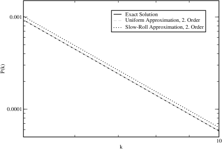
Figure 3: Comparison of the exact power spectrum for power-law inflation with the uniform approximation and the slow-roll approximation in next-to-leading order. The uniform approximation and the exact solution are indistinguishable in this plot.

In addition we can compare the spectral index for power law inflation. As explained earlier, the uniform approximation leads to the exact answer for the spectral index in the case of constant $\nu$. The slow-roll answer for power law inflation up to second order in slow-roll parameters is given by

$$n_{S}^{SR}=1-\frac{2}{p}-\frac{2}{p^{2}}.$$ (117)

For the case $p=2$, the slow-roll approximation clearly does not lead to a good answer, as the exact result is $n_{S}=-1$ while the slow-roll answer is $n_{S}=-0.5$. Of course $p=2$ does not represent a realistic model for inflation. At higher values of $p$ the slow-roll answer improves dramatically, nevertheless, unlike the uniform approximation, it is never exact. (The amplitude of the power spectrum in slow-roll approximation also improves rapidly for larger values of $p$.)

The remarkable feature of the uniform approximation is that the error in the leading order result for the solution itself (and therefore for the power spectrum) is always $\sim 8\%$, while the next-to-leading order error is less than 1%, independent of the choice of $p$. This robustness of the error control is a key feature of the uniform approximation.

VIII Comments on Bessel Function Approximants

Before concluding we would like to make another comparison to the commonly used procedure involving Bessel functions as approximating solutions for the fundamental wave equation. Recall that this approximation arises by assuming that $\nu(\eta)$ is ”locally” constant, and it forms the basis for methods discussed previously in the literature wms .

From the standpoint of the Olver uniform theory, it turns out that Bessel function approximants arise naturally when treating the case of an ODE having a coefficient function with a pole of order two Olver . Since such a pole arises in the model equation at hand, one might ask if this theory is not better suited to the computation of the power spectrum, perhaps thereby making a connection to the methods already known in the literature.

In fact, direct computation of the first order term in the Olver theory with Bessel approximants shows that it is not possible to obtain a reliable power spectrum in this way. The failure of the method is essentially due to the failure of the matching procedure at early times, $\eta\rightarrow-\infty$. This failure arises because the Bessel approximants, although uniformly controlled in $\eta$, lose too much of the more delicate $k$-dependence of the solution at large $\eta$, notably for small $k$. Following Olver’s discussion of the relation between the Bessel approximants and the Born approximation in quantum mechanics Olver , another way to state the problem is to note that the Born approximation will always fail for sufficiently low energy. In essence, Bessel approximants provide a systematic way to calculate the power spectrum at high $k$, whereas we need information at low $k$.

The success of the Airy approximants is a result of a tradeoff. By concentrating on the turning point at the expense of some early and late time information, the Airy approximants provide a successful bridge for the matching operation which is required. One of the costs of this tradeoff is a non-vanishing error in the limit $\eta\rightarrow 0$, whereas the Bessel approximants have a vanishing error in this limit. However, the error of the Bessel approximants is not sufficiently controlled in the other limit, $\eta\rightarrow-\infty$, for small $k$. Furthermore, we have shown above how the bulk of the non-vanishing contribution to the error for the Airy approximants gives rise to a $k$-independent amplitude correction, which cannot effect the spectral index; this significantly improves a priori expectations for the uniform Airy-approximation.

IX Conclusion

In this paper we have presented the uniform approximation as an excellent technique for obtaining power spectra and spectral indices from inflation models, making only a minimum number of dynamical assumptions: the answers are stated in terms of elementary functions and simple integrals which are easy to evaluate numerically. The existence of calculable and robust error bounds is a crucial advantage of the method.

In order to completely utilize this approach, the next step is a fast numerical implementation, now in progress shetal . Combined with a numerical code like CMBFAST cmbfast which translates primordial fluctuations into the linear radiation and matter power spectra, and with our now fully developed error analysis, such a capability promises to be very useful for obtaining both forward predictions from specific models as well as backward constraints from observational data.

X Acknowledgements

We thank Fabio Finelli and Ewan Stewart for helpful discussions. SH and KH acknowledge the Aspen Center for Physics where part of this work was completed. AH gratefully acknowledges Los Alamos National Laboratory for warm hospitality and thanks the Graduiertenkolleg “Physics of Elementary Particles at Accelerators and in the Universe” for partial financial support. CM-P thanks the Nuffield Foundation for partial financial support.

Appendix A Gauge-invariant Perturbations

In order to fix notation and to introduce the main equation of interest, we summarize results from cosmological perturbation theory which are of direct interest for inflationary models. The basic formalism is that of Bardeen givb ; see Ref. ivrevs2 for a detailed discussion based on this formalism.

A homogeneous and isotropic Friedmann-Robertson-Walker (FRW) universe is described by the metric

$$ds^{2} = g_{ab}dx^{a}dx^{b}$$ (118)

$$= [-dt^{2}+a^{2}(t)\gamma_{ij}(\vec{x})dx^{i}dx^{j}]$$

$$= a^{2}(\eta)[-d\eta^{2}+\gamma_{ij}(\vec{x})dx^{i}dx^{j}],$$

where $\gamma_{ij}$ is the metric on homogeneous and isotropic spatial sections, and the conformal time is $\eta=\int^{t}dt^{\prime}/a(t^{\prime})$. Let $D_{i}$ be the covariant derivative on the spatial sections. Latin letters denote spatial indices. Considering only so-called scalar and tensor perturbations, we write the perturbed metric in the form

$$ds^{2}=a(\eta)^{2}\left[ds^{2}_{S}+ds^{2}_{T}\right],$$ (119)

with the scalar and tensor perturbations

$$ds^{2}_{S} = -(1+2A)d\eta^{2}+2D_{i}Bd\eta dx^{i}$$

$$+\left[(1+2C)\gamma_{ij}+2\left(D_{i}D_{j}-\frac{1}{3}\gamma_{ij}\Delta^{\scriptscriptstyle{(3)}}\right)E\right]dx^{i}dx^{j}$$

$$ds^{2}_{T} = E_{ij}dx^{i}dx^{j}.$$ (121)

The tensor $E_{ij}$ is transverse, symmetric, and traceless. Gauge transformations of this perturbed metric are generated by vector fields of the form $\xi^{a}=(T,D^{i}L)$.

The two standard gauge invariant combinations which describe the scalar perturbations of the metric are

$$\Phi_{A} = A+(B^{\prime}+hB)-(E^{\prime\prime}+hE^{\prime}),$$ (122)

$$\Phi_{C} = C-\frac{1}{3}\Delta^{\scriptscriptstyle{(3)}}E+h(B-E^{\prime}).$$ (123)

Primes denote differentiation with respect to conformal time and $h\equiv a^{\prime}/a$. Note that in the longitudinal gauge ($L=-E$, $T=B-E^{\prime}$), the perturbed metric becomes

$$ds^{2}=a^{2}(\eta)\left[-(1+2\Phi_{A})d\eta^{2}+(1+2\Phi_{C})\gamma_{ij}dx^{i}dx^{j}\right].$$ (124)

This gauge yields a direct physical interpretation for $\Phi_{A}$ and $\Phi_{C}$. The tensor perturbations described by $E_{ij}$ are themselves gauge-invariant.

In order to complete the setup for application of the Einstein equations, we must introduce matter perturbations. The energy momentum tensor for an FRW cosmology is that of a homogeneous and isotropic perfect fluid

$$T_{ab}=\varrho(\eta)u_{a}u_{b}+p(\eta)(u_{a}u_{b}+g_{ab}),$$ (125)

where the energy density $\varrho$ and the pressure $p$ are functions only of time and $u_{a}(\eta)$ is the fluid four-velocity, which is comoving with the gravitational background, $u_{a}=-a(\eta)(d\eta)_{a}$. The most general form for the perturbation of the energy momentum tensor is

$$\delta T_{ab}=\delta\varrho u_{a}u_{b}+2aq_{(a}u_{b)}+\delta p(u_{a}u_{b}+g_{ab})+pa^{2}\Pi_{ab},$$ (126)

where $q_{a}$ is the perturbed velocity field of the fluid, and the tensor $\Pi_{ab}$ represents the anisotropies of the perturbations. The perturbations must satisfy the constraints

$$g^{ab}q_{a}u_{b}=0,\quad g^{ab}\Pi_{ab}=0,\quad\Pi^{ab}u_{b}=0.$$ (127)

Consider now the case of perturbations with vanishing anisotropic stress, $\Pi_{ab}=0$. One consequence of the Einstein equations in this case is that $\Phi\equiv\Phi_{A}=\Phi_{C}$. Further assume that the perturbations are adiabatic; then the Einstein equations can be combined to give ivrevs2

$$\Phi^{\prime\prime}+3h(1+c_{s}^{2})\Phi^{\prime}-c_{s}^{2}\Delta^{\scriptscriptstyle{(3)}}\Phi+(2h^{\prime}+(1+3c_{s}^{2})(h^{2}-\mathcal{K}))\Phi=0,$$ (128)

where $c_{s}(\eta)^{2}\equiv p^{\prime}/\varrho^{\prime}$ has the interpretation of the adiabatic sound speed squared, and $\mathcal{K}$ is the curvature of spatial sections. It turns out that if one defines $w$ by $\Phi\equiv 4\pi G(\varrho+p)^{1/2}w$, then

$$w^{\prime\prime}-c_{s}^{2}\Delta^{\scriptscriptstyle{(3)}}w-\frac{\theta^{\prime\prime}}{\theta}w=0,$$ (129)

where

$$\theta=\left(\frac{3}{2}\right)^{1/2}\frac{h}{a}\left[h^{2}-h^{\prime}+\mathcal{K}\right]^{-1/2}.$$ (130)

This is a very convenient evolution equation for the metric perturbations; it is a complete description of the dynamics of scalar perturbations, under the assumptions made on the stress tensor.

A second form of the evolution equation can be obtained by introducing a scalar $u$, which is defined by the relation

$$\Delta^{\scriptscriptstyle{(3)}}w=-c_{s}(\eta)^{-2}\left(\frac{d}{d\eta}+\frac{\theta^{\prime}}{\theta}\right)c_{s}(\eta)u.$$ (131)

Because of the relation between this definition and the differential operator which appears in the $w$ equation, it is not difficult to show that $u$ satisfies the evolution equation

$$u^{\prime\prime}-c_{s}(\eta)^{2}\Delta^{\scriptscriptstyle{(3)}}u-\frac{z^{\prime\prime}}{z}u=0,$$ (132)

where

$$z=\frac{a}{c_{s}h}\left(h^{2}-h^{\prime}+\mathcal{K}\right)^{1/2}.$$ (133)

Note also that these definitions relate the quantity $u/z$ to the metric perturbation in a simple way,

$$\Delta^{\scriptscriptstyle{(3)}}\Phi=-(4\pi G)^{1/2}\frac{h^{2}-h^{\prime}+\mathcal{K}}{hc_{s}^{2}}\left(\frac{u}{z}\right)^{\prime}.$$ (134)

Recalling that $\Phi$ has the interpretation of the Newtonian gravitational potential, this Poisson equation indicates how $u/z$ acts as a source for the potential.

Finally we specialize to the situation where the background is dominated by the dynamics of a scalar field; the only ingredient that we need from this choice is the stiff nature of a relativistic field, $c_{s}=1$. We also choose flat spatial sections as appropriate for generic inflationary models, $\mathcal{K}=0$. Since $u$ has a canonical Hamiltonian evolution, it is a natural choice for canonical quantization; the operator is expanded in terms of mode functions as in Eqn. (3), and the mode functions $u_{k}$ are found to satisfy Eqn. (4).

The tensor perturbations are expanded in terms of tensorial modes on the spatial sections,

$$E_{ij}(\eta,\mathbf{x})=\frac{1}{a}\int\mathrm{d}\mu(\mathbf{k})\;v_{k}(\eta)\mathcal{Y}_{ij}(\mathbf{x}),$$ (135)

where the mode functions $\mathcal{Y}_{ij}(\mathbf{x})$ have the properties

$$(\Delta^{\scriptscriptstyle{(3)}}+k^{2}){\cal Y}_{ij}=0,\quad\gamma^{ij}\mathcal{Y}_{ij}=0,\quad D^{i}{\cal Y}_{ij}=0.$$ (136)

Again it is found that the mode functions $v_{k}$ satisfy a simple evolution equation, which is given by Eqn. (5).

Appendix B Definition of the Errors

A key advantage of the uniform approximations presented in Ref. Olver is the uniform control over the remainder terms for the approximations. This uniform control is obtained by carefully separating the dominant influences in the coefficient functions of the ODE. Because of this uniform control, this approach is superior to the earlier results of Langer (for a good description see Ref. BO ). Additionally, Olver constructs higher order approximations not present in the original work. In this appendix we review in detail the general error formulae given by Olver. The errors in Eqns. (III) and (III) are bounded by

$$\frac{|\epsilon_{2n+1,\scriptscriptstyle\lessgtr}^{(1)}(b,\xi)|}{M(b^{2/3}\xi)},\frac{|\partial\epsilon_{2n+1,\scriptscriptstyle\lessgtr}^{(1)}(b,\xi)/\partial\xi|}{b^{2/3}N(b^{2/3}\xi)}$$ (137)

$$\leq 2E^{-1}(b^{2/3}\xi)\exp\left\{\frac{2\lambda{\cal V}_{\xi,\beta}(|\xi|^{1/2}B_{0})}{b}\right\}\frac{{\cal V}_{\xi,\beta}(|\xi|^{1/2}B_{n})}{b^{2n+1}},$$

$$\frac{|\epsilon_{2n+1,\scriptscriptstyle\lessgtr}^{(2)}(b,\xi)|}{M(b^{2/3}\xi)},\frac{|\partial\epsilon_{2n+1,\scriptscriptstyle\lessgtr}^{(2)}(b,\xi)/\partial\xi|}{u^{2/3}N(b^{2/3}\xi)}$$ (138)

$$\leq 2E(b^{2/3}\xi)\exp\left\{\frac{2\lambda{\cal V}_{\alpha,\xi}(|\xi|^{1/2}B_{0})}{b}\right\}\frac{{\cal V}_{\alpha,\xi}(|\xi|^{1/2}B_{n})}{b^{2n+1}},$$

where $M(x)$ and $N(x)$ are modulus functions, and $E(x)$ is a weight function defined as

$$M(x) = \sqrt{2{\rm Ai}(x){\rm Bi}(x)}\mbox{ for }x\leq c,$$

$$M(x) = \sqrt{{\rm Ai}^{2}(x)+{\rm Bi}^{2}(x)}\mbox{ for }x\geq c,$$ (139)

$$N(x) = \left\{\frac{{\rm Ai^{\prime}}^{2}(x){\rm Bi}^{2}(x)+{\rm Bi^{\prime}}^{2}(x){\rm Ai}^{2}(x)}{{\rm Ai}(x){\rm Bi}(x)}\right\}^{1/2}\mbox{ for }x\geq c,$$

$$N(x) = \left\{{\rm Ai^{\prime}}^{2}(x)+{\rm Bi^{\prime}}^{2}(x)\right\}^{1/2}\mbox{ for }x\leq c,$$ (140)

$$E(x) = \sqrt{\frac{{\rm Bi}(x)}{{\rm Ai}(x)}}\mbox{ for }c\leq x\leq\infty,$$

$$E(x) = 1\mbox{ for }-\infty\leq x\leq c,$$ (141)

and $c\simeq-0.36605$. Some explicit numerical values of these functions are given in Ref. Olver . The auxiliary quantity $\lambda$ is defined by

$$\lambda=\sup_{(-\infty,\infty)}\left\{\pi|x|^{1/2}M^{2}(x)\right\}.$$ (142)

A numerical estimate for $\lambda$ is $\lambda\simeq 1.04$ Olver . Finally, in Eqns. (137) and (B), we introduced the total variation of a function over the interval $(\alpha,\beta)$, ${\cal V}_{\alpha,\beta}(f)$. The total variation of a function $f(x)$ over an interval $(\alpha,\beta)$ is the supremum

$$\mathcal{V}_{\alpha,\beta}(f)=\sup_{\{\alpha\leq x_{0}<\dots<x_{n}<\dots\leq\beta\}}\sum_{s=0}^{n-1}|f(x_{s+1})-f(x_{s})|,$$ (143)

for unbounded $n$ and all possible subdivisions of the interval, $\alpha\leq x_{0}<\dots<x_{n}\leq\beta$. In case of a compact interval $[\alpha,\beta]$ one possible subdivision is given by $n=1$, $x_{0}=a$, and $x_{1}=b$. Hence

$${\cal V}_{\alpha,\beta}(f)\geq|f(\beta)-f(\alpha)|.$$ (144)

Equality holds when $f(x)$ is monotonic over $[\alpha,\beta]$. When $f(x)$ is continuously differentiable in $[\alpha,\beta]$ we have

$${\cal V}_{\alpha,\beta}(f)=\int_{\alpha}^{\beta}|f^{\prime}(x)|dx.$$ (145)

References

- (1) C.B. Netterfield et al., ApJ 571, 604 (2002); N.W. Halverson et al., ApJ 568, 38 (2002); A. Benoit et al., AA 399, L19 (2003); T.J. Pearson et al., ApJ 591, 556 (2003); C.L. Bennett et al. ApJS 148, (2003); Chao-lin Kuo et al., ApJ 600, 32 (2004).
- (2) For a review of CMB anisotropies, see W. Hu and S. Dodelson, Ann. Rev. Astron. and Astrophys. 40, 171 (2002).
- (3) e.g., W.J. Percival et al., MNRAS 327, 1297 (2001); K. Abazajian et al., AJ (to appear), astro-ph/0403325.
- (4) V. Lukash, Pis’ma Zh. Eksp. Teor. Fiz. 31, 631 (1980) [JETP Lett. 31, 596 (1980)]; V.F. Mukhanov and G.V. Chibisov, Pis’ma Zh. Eksp. Teor. Fiz. 33, 549 (1981) [JETP Lett. 33, 532 (1981)]; Zh. Eksp. Teor. Phys. 83, 475 (1982) [Sov. Phys. JETP 56, 258 (1982)]; A.H. Guth and S.-Y. Pi, Phys. Rev. Lett. 49, 1110 (1982); S.W. Hawking, Phys. Lett. B 115, 295 (1982); A.A. Starobinsky, Phys. Lett. B 117, 175 (1982).
- (5) J.M. Bardeen, Phys. Rev. D 22, 1882 (1980).
- (6) For a readable account of gauge invariant perturbations, see J.M. Stewart, Class. Quant. Grav. 7, 1169 (1990).
- (7) H. Kodama and M. Sasaki, Prog. Th. Phys. Supp. 78, 1 (1984).
- (8) V.F. Mukhanov, H.A. Feldman, and R.H. Brandenberger, Phys. Rep. 215, 203 (1992).
- (9) J.M. Bardeen, P.J. Steinhardt, and M.S. Turner, Phys. Rev. D 28, 679 (1983).
- (10) V.F. Mukhanov, JETP Letters 41, 493 (1985); Sov. Phys. JETP 68, 1297 (1988).
- (11) D.H. Lyth, Phys. Rev. D 31, 1792 (1985).
- (12) E. Lidsey, A.R. Liddle, E.W. Kolb, E.J. Copeland, T. Barreiro, and M. Abney, Rev. Mod. Phys. 69, 373 (1997).
- (13) A.R. Liddle and D.H. Lyth Cosmological Inflation and Large-Scale Structure (Cambridge, 2000) and references therein.
- (14) P.J.E. Peebles and J.T. Yu, Ap. J. 162, 815 (1970); R.A. Sunyaev and Ya.B. Zeldovich, Ap&SS 7, 3 (1970) treated the case of scalar perturbations, while the tensor case was considered in Ref. gravbg below.
- (15) A.A. Starobinskii, Pis’ma Astron. Zh. 11, 323 (1985) [Sov. Astron. Lett. 11, 133 (1985)].
- (16) W. Hu and M. White, New Astron. 2, 323 (1997).
- (17) H.M. Hodges and G.R. Blumenthal, Phys. Rev. D 42, 3329 (1990); E.J. Copeland, E.W. Kolb, A.R. Liddle, and J.E. Lidsey, Phys. Rev. D 48, 2529 (1993); 49, 1840 (1994); S. Dodelson, W.H. Kinney, and E.W. Kolb, Phys. Rev. D 56, 3207 (1997); E.J. Copeland, I.J. Grivell, E.W. Kolb, and A.R. Liddle, Phys. Rev. D 58, 043002 (1998).
- (18) M.B. Hoffman and M.S. Turner, Phys. Rev. D 64, 023506 (2001); W.H. Kinney, Phys. Rev. D 66, 083508 (2002); W.H. Kinney and R. Easther, Phys. Rev. D 67, 043511 (2003); S.M. Leach and A.R. Liddle, Phys. Rev. D 68, 123580 (2003).
- (19) S.M. Leach, A.R. Liddle, J. Martin, and D.J. Schwarz, Phys. Rev. D 66, 023515, (2002).
- (20) J. Khoury, B.A. Ovrut, P.J. Steinhardt, and N. Turok, Phys. Rev. D 64, 123522 (2001); P.J. Steinhardt and N. Turok, Phys. Rev. D 65, 126003 (2002).
- (21) E. Harrison, Phys. Rev. D 1, 2726 (1970); Ya.B. Zeldovich, MNRAS 160, 1 (1972).
- (22) R. Davis et al, Phys. Rev. Lett. 69, 1856 (1992); D. Lyth and A. Liddle, Phys. Lett. B 291, 391 (1992).
- (23) L. Wang, V.F. Mukhanov, and P.J. Steinhardt, Phys. Lett. B 414, 18 (1997).
- (24) J. Martin and D.J. Schwarz, Phys. Rev. D 62, 103520 (2000).
- (25) E.D. Stewart, Phys. Rev. D 65, 103508 (2002).
- (26) D.J. Schwarz, C.A. Terrero-Escalante, and A.A. Garcia, Phys. Lett. B 517, 243 (2001).
- (27) S. Habib, K. Heitmann, G. Jungman, and C. Molina-París, Phys. Rev. Lett. 89, 281301 (2002).
- (28) J. Martin and D.J. Schwarz, Phys. Rev. D 57, 3302 (1998).
- (29) F.W.J. Olver, Asymptotics and Special Functions, (AKP Classics, Wellesley, MA 1997).
- (30) J. Martin and D.J. Schwarz, Phys. Rev. D 67, 083512, (2003).
- (31) S.A. Fulling, Ch. VII, Aspects of Quantum Field Theory in Curved Space-Time (Cambridge University Press, New York, 1989).
- (32) S. Habib et al., in preparation.
- (33) A.H. Guth and S.Y. Pi, Phys. Rev. Lett. 49, 1110, (1982).
- (34) E.D. Stewart and J.-O. Gong, Phys. Lett. B 510, 1 (2001).
- (35) E.D. Stewart and D.H. Lyth, Phys. Lett. B 302, 171 (1993).
- (36) A.R. Liddle, P. Parsons, and J.D. Barrow, Phys. Rev. D 50, 7222 (1994).
- (37) J. Choe, J.O. Gong, and E.W. Stewart, hep-ph/0405155.
- (38) http://www.cmbfast.org; U. Seljak and M. Zaldarriaga, Ap. J. 469, 437 (1996).
- (39) C.M. Bender and S.A. Orszag Advanced Mathematical Methods for Scientists and Engineers (McGraw-Hill, 1978).