THE 24µm SOURCE COUNTS IN DEEP SPITZER SURVEYS

Abstract

Galaxy source counts in the infrared provide strong constraints on the evolution of the bolometric energy output from distant galaxy populations. We present the results from deep 24µm imaging from Spitzer surveys, which include $\approx 5\times 10^{4}$ sources to an 80% completeness of $\simeq 60$ $\mu$Jy. The 24µm counts rapidly rise at near–Euclidean rates down to 5 mJy, increase with a super–Euclidean rate between $0.4-4$ mJy, and converge below $\sim 0.3$ mJy. The 24 µm counts exceed expectations from non–evolving models by a factor $\gtrsim 10$ at $S_{\nu}\sim 0.1$ mJy. The peak in the differential number counts corresponds to a population of faint sources that is not expected from predictions based on 15$\mu$m counts from ISO. We argue that this implies the existence of a previously undetected population of infrared–luminous galaxies at $z\sim 1-3$. Integrating the counts to $60$ $\mu$Jy, we derive a lower limit on the 24µm background intensity of $1.9\pm 0.6$ nW m^-2 sr^-1 of which the majority ($\sim 60$%) stems from sources fainter than 0.4 mJy. Extrapolating to fainter flux densities, sources below $60$ $\mu$Jy contribute $0.8^{+0.9}_{-0.4}$ nW m^-2 sr^-1 to the background, which provides an estimate of the total 24 µm background of $2.7^{+1.1}_{-0.7}$ nW m^-2 sr^-1.

1. Introduction

From the first detections of infrared (IR) luminous galaxies, it was clear that they represent phenomena not prominent in optically selected galaxy surveys (e.g., Rieke & Low 1972; Soifer, Neugebauer, & Houck 1987). Locally, galaxies radiate most of their emission at UV and optical wavelengths, and only about one–third at IR wavelengths ($5-1000$ µm; Soifer & Neugebauer 1991). IR number counts from ISO indicate that the IR–luminous sources have evolved rapidly, significantly faster than has been deduced from optical surveys, which implies that IR–luminous galaxies make a substantial contribution to the cosmic star–formation rate density (e.g., Elbaz et al. 1999; Franceschini et al. 2001). The detection of the cosmic background by COBE at IR wavelengths shows that the total far–IR emission of galaxies in the early Universe is greater than that at optical and UV wavelengths (Fixsen et al., 1998; Hauser et al., 1998; Madau & Pozzetti, 2000; Franceschini et al., 2001), which suggests that a large fraction of stars have formed in IR–luminous phases of galaxy activity (Elbaz et al., 2002). Studies from ISO at 15 µm and 170 µm have inferred that the bulk of this background originates in discrete sources with $z\lesssim 1.2$ (Dole et al., 2001; Elbaz et al., 2002). However, the peak in the cosmic IR background extends to $\sim 200$µm (Fixsen et al., 1998; Hauser & Dwek, 2001). The spectral–energy distributions (SEDs) of luminous IR galaxies ($L_{\mathrm{IR}}\sim 10^{11-12}$ $L_{\odot}$) peak between $50-80$ µm (Dale et al., 2001). If these objects constitute a major component of the cosmic IR background, then it follows there is a significant population of IR–luminous galaxies at $z\sim 1.5-3$ — distances largely unexplored by ISO.

Table 1Properties of Deep, Spitzer Fields

	R.A.	Decl.	$\langle I_{\nu}\rangle$	Area	$\langle t_{\mathrm{exp}}\rangle$	$C_{80\%}$	$N(>C_{80\%})$	$N(>300\ \mu\mathrm{Jy})$
Field	(J2000.0)	(J2000.0)	(MJy sr-1)	(arcmin2)	(sec)	($\mu$Jy)	(arcmin-2)	(arcmin-2)
(1)	(2)	(3)	(4)	(5)	(6)	(7)	(8)	(9)
Marano	$03\ 13\ 52$	$-55\ 15\ 23$	19.7	01296	0236	170	2.0	0.9
CDF–S	$03\ 32\ 28$	$-27\ 48\ 30$	22.5	02092	1378	083	4.5	0.7
EGS	$14\ 16\ 00$	$+52\ 48\ 50$	19.5	01466	0450	110	3.4	0.7
Boötes	$14\ 32\ 06$	$+34\ 16\ 48$	22.7	32457	0087	270	1.0	0.8
ELAIS	$16\ 09\ 52$	$+54\ 55\ 00$	18.2	00130	3232	061	5.7	0.6

Note. — Col. (1) Field name; (2) right ascension in units of hours, minutes, and seconds; (3) declination in units of degrees, arcminutes, and arcseconds; (4) mean 24 µm background; (5) areal coverage; (6) mean exposure time; (7) 80% completeness limit; (8) source density with $S_{\nu}>C_{80\%}$. (9) source density with $S_{\nu}>300$ $\mu$Jy.

The mid–IR 24 µm band on the Multiband Imaging Photometer for Spitzer (MIPS, Rieke et al., 2004) is particularly well suited for studying distant IR–luminous galaxies. Locally, the mid–IR emission from galaxies relates almost linearly with the total IR luminosity over a range of galaxy types (e.g., Spinoglio et al., 1995; Chary & Elbaz, 2001; Roussel et al., 2001; Papovich & Bell, 2002), and there are indications this holds at higher redshifts (e.g., Elbaz et al., 2002). Because the angular resolution of Spitzer is significantly higher for the 24 µm band relative to 70 and 160 µm, the 24 µm confusion limit lies at fainter flux densities. This allows us to probe the IR emission from many more sources and at higher redshifts than with the MIPS longer wavelength bands (e.g., Papovich & Bell, 2002; Dole et al., 2003). Here, we present the number counts of $\approx 5\times 10^{4}$ sources detected at 24 µm in deep Spitzer surveys, and we suggest that the faint Spitzer detections probe a previously undetected population of very luminous galaxies at high redshifts. Where applicable, we assume $\Omega_{m}=0.3$, $\Omega_{\Lambda}=0.7$, and $H_{0}=70$ km s^-1 Mpc^-1.

2. The Data and Source Samples

The data used in this work were obtained in five fields from early Spitzer characterization observations and from time allocated to the MIPS Guaranteed Time Observers (GTOs). Table 1 lists their properties and 24 µm source densities. The MIPS fields used here subtend the largest areas ($\simeq 10.5$ deg²) and widest range in flux density ($50-0.06$ mJy) available to date from the Spitzer mission, and therefore are the premier dataset for studying the mid–IR source counts.

The MIPS 24 µm images were processed with the MIPS GTO data analysis tool (Gordon et al., 2004). The measured count rates are corrected for dark current, cosmic–rays, and flux nonlinearities, and then divided by flat–fields for each MIPS scan–mirror position. Images are then corrected for geometric distortion and mosaicked. The final mosaics have a pixel scale of $\simeq 1\farcs 25$ pix^-1, with a point–spread function (PSF) full–width at half maximum (FWHM) of $\simeq 6\arcsec$.

Figure 1.— Reliability of source detection and photometry for the CDF–S, one of the deep Spitzer fields. The thick line shows the fraction of artificial sources detected in the image as a function of input flux density. For the CDF–S this fraction is 80% complete at $C_{80\%}=83$ $\mu$Jy (indicated by the dotted line). The red line shows the ratio of the number of sources detected in a ‘negative’ of the 24µm image to the number of ‘positive’ sources as a function of flux density, which provides an estimate of the number of spurious sources due to noise features.

We performed source detection and photometry using a set of tools and simulations. Briefly, we first subtract the image background using a median filter roughly four times the size of source apertures (see below), and use a version of the DAOPHOT software (Stetson, 1987) to detect point sources. We filter each image with a Gaussian with a FWHM that is equal to that of the MIPS 24 µm PSF, and identify positive features in 10″–diameter apertures above some noise threshold. We then construct empirical PSFs using $20-30$ bright sources in each image, and optimally measure photometry by simultaneously fitting the empirical PSFs to all sources within $\simeq 20$″ of nearby object centroids. The source photometry corresponds to the flux of these PSF–apertures within a diameter of $37\farcs 4$, and we apply a multiplicative correction of 1.14 to account for light lost outside these apertures.

Figure 2.— Cumulative (Left panel) and differential (Right panel) 24µm number counts. The differential counts have been normalized to a Euclidean slope, $dN/dS_{\nu}\sim S_{\nu}^{-2.5}$. The solid stars show the average counts from all the Spitzer fields (see Table 1), and corrected for completeness to their respective 80% limits. The open star corresponds to counts brighter than the 50% completeness limit from the ELAIS field. The error bars correspond to counting uncertainties and a cosmic–variance estimate based on the standard deviation of the field–to–field counts from the different fields. Each flux bin is $\Delta(\log S_{\nu})=0.15$ dex. The shaded diamonds correspond to IRAS 25 µm number counts from Hacking & Soifer (1991, and adjusted assuming $\nu_{24}S_{\nu}(24\micron)=\nu_{25}S_{\nu}(25\micron)$). The curves show the predictions from various contemporary models from the literature (see figure inset; and adjusted slightly to match the observed IRAS counts), and a model based on the local ISO 15µm luminosity function and assuming non–evolving galaxy SEDs.

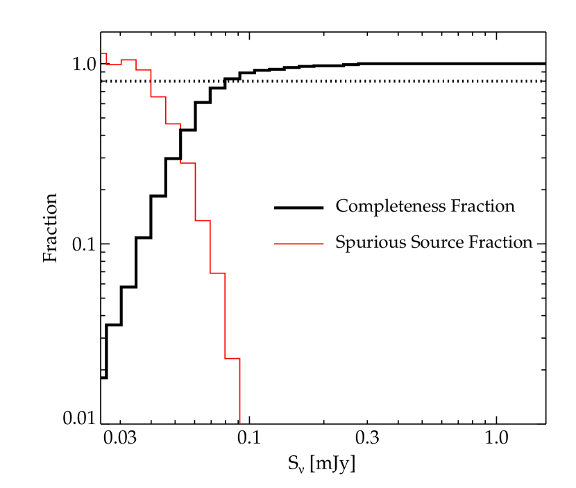
To estimate completeness and photometric reliability in the 24 µm source catalogs, we repeatedly inserted artificial sources into each image with a flux-distribution approximately matching the measured number counts. We then repeated the source detection and photometry process, and compared the resulting photometry to the input values. In figure 1, we show for the Chandra Deep Field South (CDF–S; one of the deep, Spitzer fields) the relative fraction of sources within $r\leq 2\farcs 3$ (half the FWHM) and with a flux difference $<50$% compared to their input values. From these simulations, we estimated the flux–density limit where 80% of the input sources are recovered with this photometric accuracy, and these are listed in table 1. Simultaneously, we estimate that down to the 80% completeness limit the number of sources that result from fainter sources either by photometric errors or the merging of real sources is $\lesssim 10$%. We also repeated the source detection and photometry process on the negative of each MIPS 24 µm image. This test provides an estimate for the number of spurious sources arising from the noise properties of the image, as shown in figure 1. For all of our fields, the spurious–source fraction for flux densities greater than the 80% completeness limit is $<10$%.

3. The 24 µm Source Counts

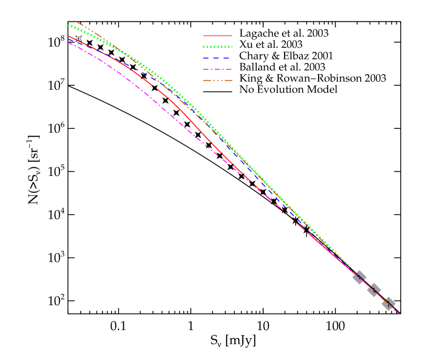
Figure 2 shows the 24 µm cumulative and differential number counts that have been averaged over the fields listed in table 1. The differential and cumulative counts (corrected and uncorrected) are listed in table 2. The faintest datum (denoted by the open symbol in figure 2) is derived to the 50% completeness limit for the European Large–Area ISO Survey (ELAIS) field ($C_{50\%}=35$ $\mu$Jy). The remaining (less deep) fields are used after correcting for completeness to the 80% level only. Error bars in the figure correspond to Poissonian uncertainties and an estimate for cosmic variance using the standard deviation of counts between the fields. For $S_{\nu}\leq 83$ $\mu$Jy where the counts are derived solely from the smaller ELAIS field, we estimate the uncertainty (18%) using the standard deviation of counts at faint flux densities in cells of 130 arcmin² from the CDF–S (see below). We have ignored the contribution to the number counts from stars at 24 µm, which are negligible at these Galactic latitudes and flux densities based on preliminary Spitzer observations.

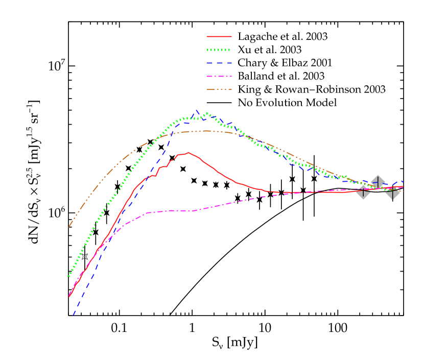
At bright flux densities, $S_{\nu}\gtrsim 5$ mJy, the differential 24 µm source counts increase at approximately the Euclidean rate, $dN/dS_{\nu}\sim S^{-2.5}$, which extends the trends observed by the IRAS 25 µm population by two orders of magnitude (Hacking & Soifer, 1991; Shupe et al., 1998). For $S_{\nu}\simeq 0.4-4$ mJy, the 24 µm counts increase at super–Euclidean rates, and peak near $0.2-0.4$ mJy. This observation is similar to the trend observed in the ISO 15 µm source counts (Elbaz et al., 1999), but the peak in the 24 µm differential source counts occurs at fluxes fainter by a factor $\approx 2.0$. The peak lies above the 80% completeness limit for nearly all fields, and is seen in the counts of the fields individually. Thus the observed turn over is quite robust. The counts converge rapidly with a sub–Euclidean rate at $\lesssim 0.2$ mJy. We broadly fit the faint–end ($S_{\nu}\simeq 35-130$ $\mu$Jy) of the differential number counts using a powerlaw, $dN/dS_{\nu}=C\,(S_{\nu}/1\,\mathrm{mJy})^{-\alpha}$, with $\alpha=-1.5\pm 0.1$. This result is consistent with a separate analysis based solely on the ELAIS field (Chary et al., 2004).

The observed counts are strongly inconsistent with expectations from non–evolving models of the local IR–luminous population. In figure 2, we show the 24 µm counts derived from the local luminosity function at ISO 15 µm (Xu, 2000) and assuming local galaxy SEDs (Dale et al., 2001). We have used the the local ISO 15 µm luminosity function, because the $k$–correction between rest–frame ISO 15 µm and observed MIPS 24 µm bands is minimized at higher redshifts ($z\sim 0.6$), which is more appropriate for the counts at fainter flux densities. However, using the local IRAS 25 µm luminosity function (Shupe et al., 1998) yields essentially identical results. While the non–evolving fiducial model is consistent with the observed 24 µm counts for $S_{\nu}\gtrsim 20$ mJy, it underpredicts the counts at $S_{\nu}\lesssim 0.4$ mJy by more than a factor of 10.

Because the deep Spitzer fields are measured in many sightlines with large solid angle, we can estimate the fluctuations in the number of sources as a function of sky area and flux density in smaller–sized fields. For example, in the CDF–S, which achieves an 80%–completeness limit of 83 $\mu$Jy over $\simeq 0.6$ deg² (see table 1 and figure 1), we have computed the variance in the number of sources in solid angles of 100 and 300 arcmin². For the sources that span the peak in the differential counts ($0.1-1$ mJy), the fluctuation in the number of sources in flux–density bins of 0.15 dex is roughly $15$% in these areas. This implies that small–sized fields suffer sizable field–to–field variation in the number of counts from the cosmic variance of source clustering. This effect is present in even larger fields: the number density of sources brighter than 0.3 mJy varies by $\sim 10$% in fields of $\sim 0.5$ deg² (table 1), and is consistent with fluctuations expected from galaxy clustering on fields of this size at $z\sim 1$, (scale lengths of $20-70$ Mpc). The counts presented here average over fields from many sightlines and significantly larger areas. We conservatively estimate that variations due to galaxy clustering correspond to uncertainties in the number counts of a less than a few percent in each flux bin.

4. Interpretation and Discussion

The form of the observed 24 µm source counts differs strongly from predictions of various contemporary models (see figure 2). Four of the models are phenomenological in approach, which parameterize the evolution of IR–luminous galaxies in terms of density and luminosity to match observed counts from ISO, radio, sub–mm, and other datasets. Several of these models (Chary & Elbaz, 2001; King & Rowan–Robinson, 2003; Xu et al., 2003) show a rapid increase in the number of sources at super–Euclidean rates at relatively bright flux densities ($S_{\nu}\gtrsim 10$ mJy) and peak near 1 mJy. These models generally predict a redshift distribution for the MIPS 24 µm population that peaks near $z\sim 1$, based largely on expectations from the ISO populations, and they overpredict the 24 µm number counts by factors of $2-3$ at $\sim 1$ mJy. The Lagache et al. (2003) model predicts a roughly Euclidean increase in the counts for $S_{\nu}>10$ mJy. The shape of the counts in this model is similar to the observed distribution, but it peaks at $S_{\nu}\sim 1$ mJy, at higher flux densities than the observed counts. This model predicts a redshift distribution that peaks near $z\sim 1$, but tapers slowly with a significant population of IR–luminous galaxies out to $z\gtrsim 2$ (Dole et al., 2003).

The model of Balland, Devriendt, & Silk (2003) is based on semi–analytical hierarchical models within the Press–Schecter formalism in which galaxies identified as ‘interacting’ are assigned IR–luminous galaxy SEDs. This model includes additional physics in that the evolution of galaxies depends on their local environment and merger/interaction histories. Although this model predicts a near–Euclidean increase in the counts for $S_{\nu}\gtrsim 10$ mJy, the counts shift to sub–Euclidean rates at relatively bright flux densities. The semi–analytical formalism seems to not include important physics that are necessary to reproduce the excess of faint IR sources. This illustrates the need for large–area multi–wavelength studies of Spitzer sources to connect optical– and IR–selected sources at high redshift to understand the mechanisms that produce IR–luminous stages of galaxy evolution.

The peak in the 24 µm differential number counts occurs at fainter flux densities than predicted from the phenomenological models based on the ISO results. This may suggest possibilities such as a steepening in the slope of the IR luminosity function with redshift, or evolution in the relation between the mid– and total IR. Phenomenological models which reproduce the IR background predict a faint–end slope of the IR luminosity function that should be quite shallow at high redshifts, with ‘$L^{\ast}$’ luminosities that correspond to $L_{\mathrm{IR}}>10^{11}$ $L_{\odot}$ for $z\gtrsim 1$ (see Hauser & Dwek, 2001). For most plausible IR luminosity functions, galaxies with $L^{\ast}$ luminosities dominate the integrated luminosity density. Elbaz et al. (2002) observed that the redshift distribution of objects with these luminosities in deep ISO surveys spans $z\simeq 0.8-1.2$, and that these objects constitute a large fraction of the total cosmic IR background. Therefore, it seems logical that objects with these luminosities dominate 24 µm number counts at $0.1-0.4$ mJy, and it follows that their redshift distribution must lie at $z\sim 1-3$ (i.e., where this flux density corresponds to $\sim 10^{11-12}$ $L_{\odot}$, using empirical relations from Papovich & Bell 2002). Indeed, a similar conclusion is inferred based on a revised phenomenological model using the 24 µm number counts presented here (Lagache et al., 2004), and allowing for small changes in the mid–IR SEDs of IR–luminous galaxies. Examples of MIPS 24 µm sources at these redshifts and luminosities have been readily identified in optical ancillary data (Le Floc’h et al., 2004). We therefore attribute the the peak in the 24 µm differential number counts at fainter flux densities to a population of luminous IR galaxies at redshifts higher than explored by ISO.

Integrating the differential source–count distribution provides an estimate for their contribution to the cosmic IR background at 24 µm, i.e, $I_{\nu}=\int dN/dS_{\nu}\,S_{\nu}\,dS_{\nu}$. For sources brighter than 60 $\mu$Jy, we derive a lower limit on the total background of $\nu I_{\nu}(24\micron)=1.9\pm 0.6$ nW m^-2 sr^-1. Due to the steep nature of the source counts, most of this background emission results from galaxies with fainter apparent flux densities. We find that $\simeq 60$% of the 24 µm background originates in galaxies with $S_{\nu}\leq 0.4$ mJy, and therefore the galaxies responsible for the peak in the differential source counts also dominate the total background emission. Our result is consistent with the COBE DIRBE upper limit $\nu\,I_{\nu}(25\micron)<7$ nW m^-2 sr^-1 inferred from fluctuations in the IR background (Kashlinsky & Odenwald, 2000; Hauser & Dwek, 2001). As a further estimate on the total 24 µm background intensity, we have extrapolated the number counts for $S_{\nu}<60$ $\mu$Jy using the fit to the faint–end slope of the 24 µm number counts in § 3. Under this assumption, we find that sources with $S_{\nu}<60$ $\mu$Jy would contribute $0.8^{+0.9}_{-0.4}$ nW m^-2 sr^-1 to the 24 µm background, which when summed with the above measurement yields an estimate of the total background of $\nu I_{\nu}^{(\mathrm{tot})}(24\micron)=2.7^{+1.1}_{-0.7}$ nW m^-2 sr^-1. For this value, the sources detected in the deep Spitzer 24 µm surveys produce $\sim 70$% of the total 24 µm background.

Table 2Measured Spitzer 24 $\mu\mathrm{m}$ Number Counts

Log $S_{\nu}$	$dN/dS_{\nu}$	$\delta(dN/dS_{\nu})$	Log $S_{\nu}$	$N(>S_{\nu})$	$\delta(N(>S_{\nu}))$
(mJy)	(mJy-1 sr-1)	(mJy-1 sr-1)	(mJy)	(sr-1)	(sr-1)
(1)	(2)	(3)	(4)	(5)	(6)
$-1.475$	2.5 (1.4) $\times 10^{9}$	4.7 (1.5) $\times 10^{8}$	$-1.550$	2.1 (1.1) $\times 10^{8}$	1.2 (0.60) $\times 10^{7}$
$-1.325$	1.5 (1.2) $\times 10^{9}$	2.7 (0.97) $\times 10^{8}$	$-1.400$	1.2 (0.92) $\times 10^{8}$	7.6 (4.9) $\times 10^{6}$
$-1.175$	8.7 (6.9) $\times 10^{8}$	1.4 (1.4) $\times 10^{8}$	$-1.250$	9.6 (7.2) $\times 10^{7}$	3.7 (0.68) $\times 10^{6}$
$-1.025$	5.5 (5.2) $\times 10^{8}$	5.8 (1.6) $\times 10^{7}$	$-1.100$	6.1 (5.6) $\times 10^{7}$	5.9 (5.6) $\times 10^{5}$
$-0.875$	3.1 (3.1) $\times 10^{8}$	7.1 (4.9) $\times 10^{6}$	$-0.950$	3.9 (3.9) $\times 10^{7}$	4.0 (4.0) $\times 10^{5}$
$-0.725$	1.7 (1.6) $\times 10^{8}$	7.6 (6.0) $\times 10^{6}$	$-0.800$	2.9 (2.5) $\times 10^{7}$	5.5 (5.0) $\times 10^{5}$
$-0.575$	8.3 (7.5) $\times 10^{7}$	1.5 (0.66) $\times 10^{6}$	$-0.650$	1.8 (1.6) $\times 10^{7}$	1.8 (1.6) $\times 10^{5}$
$-0.425$	$3.2\times 10^{7}$	$5.7\times 10^{5}$	$-0.500$	$8.6\times 10^{6}$	$1.2\times 10^{5}$
$-0.275$	$1.2\times 10^{7}$	$1.9\times 10^{5}$	$-0.350$	$4.4\times 10^{6}$	$6.2\times 10^{4}$
$-0.125$	$4.1\times 10^{6}$	$9.6\times 10^{4}$	$-0.200$	$2.3\times 10^{6}$	$3.8\times 10^{4}$
+$0.025$	$1.4\times 10^{6}$	$3.9\times 10^{4}$	$-0.050$	$1.2\times 10^{6}$	$2.3\times 10^{4}$
+$0.175$	$5.8\times 10^{5}$	$2.1\times 10^{4}$	+$0.100$	$7.1\times 10^{5}$	$1.7\times 10^{4}$
+$0.325$	$2.4\times 10^{5}$	$1.1\times 10^{4}$	+$0.250$	$4.1\times 10^{5}$	$1.4\times 10^{4}$
+$0.475$	$1.0\times 10^{5}$	$6.5\times 10^{3}$	+$0.400$	$2.3\times 10^{5}$	$1.0\times 10^{4}$
+$0.625$	$3.4\times 10^{4}$	$2.8\times 10^{3}$	+$0.550$	$1.3\times 10^{5}$	$7.1\times 10^{3}$
+$0.775$	$1.5\times 10^{4}$	$1.6\times 10^{3}$	+$0.700$	$7.7\times 10^{4}$	$5.5\times 10^{3}$
+$0.925$	$6.0\times 10^{3}$	$8.6\times 10^{2}$	+$0.850$	$5.2\times 10^{4}$	$7.4\times 10^{3}$
+$1.075$	$2.7\times 10^{3}$	$4.9\times 10^{2}$	+$1.000$	$3.4\times 10^{4}$	$6.0\times 10^{3}$
+$1.225$	$1.2\times 10^{3}$	$2.7\times 10^{2}$	+$1.150$	$2.0\times 10^{4}$	$4.0\times 10^{3}$
+$1.375$	$6.2\times 10^{2}$	$1.7\times 10^{2}$	+$1.300$	$1.3\times 10^{4}$	$2.8\times 10^{3}$
+$1.525$	$2.2\times 10^{2}$	$8.3\times 10^{1}$	+$1.450$	$7.3\times 10^{3}$	$2.1\times 10^{3}$
+$1.675$	$1.1\times 10^{2}$	$5.0\times 10^{1}$	+$1.600$	$4.4\times 10^{3}$	$1.5\times 10^{3}$

Note. — Col. (1) Flux density for differential number counts; (2) Corrected differential counts and (3) uncertainty; (4) Flux density for cumulative number counts; (5) Corrected cumulative counts and (6) uncertainty. Numbers in parentheses give the uncorrected values.

References

- Balland et al. (2003) Balland, C., Devriendt, J. E. G., & Silk, J. 2003, MNRAS, 343, 107
- Chary & Elbaz (2001) Chary, R. R., & Elbaz, D. 2001, ApJ, 556, 562
- Chary et al. (2004) Chary, R. R. et al. 2004, ApJS, this issue
- Dale et al. (2001) Dale, D. A., Helou, G., Contursi, A., Silbermann, N. A., & Kolhatkar, S. 2001, ApJ, 549, 215
- Dole et al. (2001) Dole, H., et al. 2001, A&A, 372, 364
- Dole et al. (2003) Dole, H., Lagache, G., & Puget, J.–P. 2003, ApJ, 585, 617
- Elbaz et al. (1999) Elbaz, D., et al. 1999, A&A, 351, L37
- Elbaz et al. (2002) Elbaz, D., Cesarsky, C. J., Chanial, P., Aussel, H., Franceschini, A., Fadda, D., & Chary, R. R. 2002, A&A, 384, 848
- Fixsen et al. (1998) Fixsen, D. J., Dwek, E., Mather, J. C., Bennett, C. L., & Shafer, R. A. 1998, ApJ, 508, 123
- Franceschini et al. (2001) Franceschini, A., Aussel, H., Cesarsky, C. J., Elbaz, D., & Fadda, D. 2001, A&A, 378, 1
- Gordon et al. (2004) Gordon, K. et al. 2004, PASP, submitted
- Hacking & Soifer (1991) Hacking, P., & Soifer, B. T. 1991, ApJ, 367, L49
- Hauser et al. (1998) Hauser, M. G., et al. 1998, ApJ, 508, 25
- Hauser & Dwek (2001) Hauser, M. G. & Dwek, E. 2001, ARA&A, 39, 249
- Kashlinsky & Odenwald (2000) Kashlinsky, A. & Odenwald, S. 2000, ApJ, 528, 74
- King & Rowan–Robinson (2003) King, A. J., & Rowan–Robinson, M. 2003, MNRAS, 339, 260
- Lagache et al. (2003) Lagache, G., Dole, H., & Puget, J.–L. 2003, MNRAS, 338, 555
- Lagache et al. (2004) Lagache, G., et al. 2004, ApJS, this issue
- Le Floc’h et al. (2004) Le Floc’h, E. et al. 2004, ApJS, this issue
- Madau & Pozzetti (2000) Madau, P. & Pozzetti, L. 2000, MNRAS, 312, 9
- Papovich & Bell (2002) Papovich, C. & Bell, E. F. 2002, ApJ, 579, L1
- Rieke & Low (1972) Rieke, G. & Low, F. 1972, ApJ, 176, 95
- Rieke et al. (2004) Rieke, G. et al. 2004, ApJS, this issue
- Roussel et al. (2001) Roussel, H., Sauvage, M., Vigroux, L. & Bosma, A. 2001, A&A, 372, 427
- Shupe et al. (1998) Shupe, D. L., Fang, F., Hacking, P. B., & Huchra, J. P. 1998, ApJ, 501, 597
- Spinoglio et al. (1995) Spinoglio, L., Malkan, M. A., Rush, B., Carrasco, L., & Recillas–Cruz, E. 1995, ApJ, 453, 616
- Soifer et al. (1987) Soifer, B. T., Neugebauer, G., & Houck, J. R. 1987, ARA&A, 25, 187
- Soifer & Neugebauer (1991) Soifer, B. T., & Neugebauer, G. 1991, AJ, 101, 354
- Stetson (1987) Stetson, P. B. 1987, PASP, 99, 191
- Xu (2000) Xu, C. 2000, ApJ, 541, 134
- Xu et al. (2003) Xu, C., Lonsdale, C. J., Shupe, D. L., Franceschini, A., Martin, C., & Schiminovich, D. 2003, ApJ, 587, 90