Cross-correlation of CMB with large-scale structure: weak gravitational lensing

Abstract

We present the results of a search for gravitational lensing of the cosmic microwave background (CMB) in cross-correlation with the projected density of luminous red galaxies (LRGs). The CMB lensing reconstruction is performed using the first year of Wilkinson Microwave Anisotropy Probe (WMAP) data, and the galaxy maps are obtained using the Sloan Digital Sky Survey (SDSS) imaging data. We find no detection of lensing; our constraint on the galaxy bias derived from the galaxy-convergence cross-spectrum is $b_{g}=1.81\pm 1.92$ ($1\sigma$, statistical), as compared to the expected result of $b_{g}\sim 1.8$ for this sample. We discuss possible instrument-related systematic errors and show that the Galactic foregrounds are not important. We do not find any evidence for point source or thermal Sunyaev-Zel’dovich effect contamination.

I Introduction

The Wilkinson Microwave Anisotropy Probe (WMAP) satellite has provided a wealth of information about the universe through its high-resolution, multi-frequency, all-sky maps of the cosmic microwave background (CMB) Bennett et al. (2003a). While the WMAP power spectrum Hinshaw et al. (2003a) and temperature-polarization cross-spectrum Kogut et al. (2003) are useful for probing the high-redshift universe (reionization and earlier epochs) Spergel et al. (2003); Verde et al. (2003); Peiris et al. (2003); Page et al. (2003a), the WMAP maps also provide an opportunity to study the low-redshift universe through secondary CMB anisotropies. While the effect of secondary anisotropies on the angular scales probed by WMAP ($l\lesssim 700$) is small compared to the primordial temperature fluctuations, the signal-to-noise ratio can be boosted by cross-correlating with tracers of the large scale structure (LSS) at low redshifts. Since the WMAP data release, several authors have used various tracers of LSS to measure the integrated Sachs-Wolfe (ISW) effect, the thermal Sunyaev-Zel’dovich (tSZ) effect, and microwave point sources Diego et al. (2003); Boughn and Crittenden (2004); Nolta et al. (2004); Myers et al. (2004); Fosalba et al. (2003); Scranton et al. (2003); Afshordi et al. (2004). The Sloan Digital Sky Survey (SDSS) is an excellent candidate for these cross-correlation studies due to the large solid angle covered at moderate depth.

Another secondary anisotropy, which has not yet been investigated observationally, is weak lensing of the CMB by intervening large-scale structure. Weak lensing has attracted much attention recently as a means of directly measuring the matter power spectrum at low redshifts (e.g. Refregier (2003)). The traditional approach is to use distant galaxies as the “sources” that are lensed to measure e.g. the matter power spectrum (e.g. Van Waerbeke et al. (2000); Bacon et al. (2000); Rhodes et al. (2001); Hoekstra et al. (2002a); Van Waerbeke et al. (2002); Jarvis et al. (2003); Brown et al. (2003); Massey et al. (2004)) or the galaxy-matter cross-correlation (e.g. Brainerd et al. (1996); Fischer et al. (2000); McKay et al. (2001); Hoekstra et al. (2002b); Sheldon et al. (2004); Hoekstra et al. (2004)). However weak lensing of CMB offers an alternative method, free of intrinsic alignments, uncertainties in the source redshift distribution, and selection biases (since the CMB is a random field). Potential applications of CMB lensing described in the literature include precision measurement of cosmological parameters Hu and Okamoto (2002); Hu (2002); Kaplinghat (2003); Hu and Okamoto (2004) and separation of the lensing contribution to the CMB $B$-mode polarization from primoridal vector Lewis (2004) and tensor perturbations Knox and Song (2002); Kesden et al. (2002); Seljak and Hirata (2004). While these applications are in the future, the WMAP data for the first time allows a search for weak lensing of the CMB in correlation with large-scale structure. This paper presents the results of such a search; our objective here is not precision cosmology, but rather to detect and characterize any systematic effects that contaminate the lensing signal at the level of the current data. This step is a prerequisite to future investigations that will demand tighter control of systematics.

In this paper, we perform cross-correlation analysis between the CMB weak lensing field derived from WMAP and a photometrically selected sample of luminous red galaxies (LRGs) in the SDSS at redshifts $0.2<z<0.7$. The photometric LRGs are well-suited for cross-correlation studies because of their high intrinsic luminosity (compared to normal galaxies), which allows them to be observed at large distances; their high number density, which suppresses shot noise in the maps; and their uniform colors which allow for accurate photometric redshifts and hence determination of the redshift distribution. We use the measured cross-spectrum between the lensing field and the projected galaxy density to estimate the LRG bias $b_{g}$. At the present stage, we are using the bias as a proxy for the strength of the cross-correlation signal, just as has been done in recent analyses of the ISW effect Boughn and Crittenden (2004); Nolta et al. (2004); Fosalba et al. (2003); Scranton et al. (2003); Afshordi et al. (2004); we are not yet trying to use the bias in cosmological parameter estimation, although this is a possible future application of the methodology. We do not have a detection of a cross-correlation, and hence our measured bias $b_{g}=1.81\pm 1.92$ is consistent with zero.

This paper is organized as follows. The most important aspects (for this analysis) of the WMAP and SDSS data sets, and the construction of the LRG catalog, are described in Sec. II. The theory of CMB lensing and reconstruction methodology are explained in Sec. III. The cross-correlation methodology and simulations are covered in Sec. IV, and the results are presented in Sec. V. We investigate possible systematic errors in Sec. VI, and conclude in Sec. VII. Appendix A describes the spherical harmonic transform algorithms and associated conventions used in this paper, and Appendix B describes the algorithm used for the ${\sf C}^{-1}$ operations that arise in our analysis.

II Data

II.1 CMB temperature from WMAP

The WMAP mission Bennett et al. (2003b) is designed to produce all-sky maps of the CMB at multipoles up to $l\sim$several hundred. This analysis uses the first public release of WMAP data, consisting of one year of observations from the Sun-Earth L2 Lagrange point. WMAP carries ten differencing assemblies (DAs), each of which measures the difference in intensity of the CMB at two points on the sky; a CMB map is buit up from these temperature differences as the satellite rotates. (WMAP has polarization sensitivity but this is not used in the present analysis.) The DAs are designated K1, Ka1, Q1, Q2, V1, V2, W1, W2, W3, and W4; the letters indicate the frequency band to which a particular DA is sensitive Bennett et al. (2003a); Jarosik et al. (2003) (the K, Ka, Q, V, and W bands correspond to central frequencies of 23, 33, 41, 61, and 94 GHz, respectively). The WMAP team has pixelized the data from each DA in the HEALPix pixelization system at resolution 9 Bennett et al. (2003a); Hinshaw et al. (2003b). This system has 3,145,728 pixels, each of solid angle 47.2 sq. arcmin. These maps are not beam-deconvolved; this, combined with the WMAP scan strategy, results in nearly uncorrelated Gaussian uncertainties on the temperature in each pixel.

In this paper, we only use the three high-frequency microwave bands (Q, V, and W) because the K and Ka bands are very heavily contaminated by galactic foregrounds and have poor resolution. (The foreground emission is not a Gaussian field and cannot be reliably simulated, so in cases where it dominates over CMB anisotropy and instrument noise, we cannot compute reliable error bars on the cross-correlation.) For the galaxy-lensing correlation, we have used the sky maps produced by the eight high-frequency DAs. The variances of the temperature measurements are obtained from the effective number of observations $N_{obs}$.

Note that the WMAP “internal linear combination” (ILC) map Bennett et al. (2003a) cannot be used for lensing studies because of its degraded resolution (1 degree full width half maximum, FWHM), which eliminates the multipoles $l\sim 350$ of greatest importance for the lensing analysis. An ILC-based lensing analysis would also suffer from practical issues, namely the loss of frequency-dependent information (useful as a test of foregrounds), the inability to separate cross-correlations between different DAs from auto-correlations (useful to avoid the need for noise bias subtraction), and the complicated inter-pixel noise correlations (due to the smoothing used to create the map and the varying weights of the different frequencies). The foreground-cleaned map of Ref. Tegmark et al. (2003) recovers the full WMAP resolution, but the practical difficulties (for the purpose of lensing reconstruction) associated with ILC still apply. We have not used either of these maps in this paper.

II.2 LRG density from SDSS

The Sloan Digital Sky Survey (SDSS) York et al. (2000) is an ongoing survey to image approximately $\pi$ steradians of the sky, and follow up approximately one million of the detected objects spectroscopically Strauss et al. (2002); Richards et al. (2002). The imaging is carried out by drift-scanning the sky in photometric conditions Hogg et al. (2001), in five bands ($ugriz$) Fukugita et al. (1996); Smith et al. (2002) using a specially designed wide-field camera Gunn et al. (1998). These imaging data are the source of the LSS sample that we use in this paper. In addition, objects are targeted for spectroscopy using these data Blanton et al. (2003) and are observed with a 640-fiber spectrograph on the same telescope. All of these data are processed by completely automated pipelines that detect and measure photometric properties of objects, and astrometrically calibrate the data Lupton et al. (2001); Pier et al. (2003). The SDSS is well underway, and has had three major data releases Stoughton et al. (2002); Abazajian et al. (2003, 2004); Finkbeiner et al. (2004); this paper uses all data observed through Fall 2003 (296,872 HEALPix resolution 9 pixels, or 3,893 square degrees).

The SDSS detects many extragalactic objects that could, in principle, be used for cross-correlation with secondary anisotropies Peiris and Spergel (2000). The usefulness of LRGs as a cosmological probe has been appreciated by a number of authors Gladders and Yee (2000); Eisenstein et al. (2001). These are typically the most luminous galaxies in the universe, and therefore probe cosmologically interesting volumes. In addition, these galaxies are generically old stellar systems and have extremely uniform spectral energy distributions (SEDs), characterized only by a strong discontinuity at 4000 Å. The combination of these two characteristics make them an ideal candidate for photometric redshift algorithms, with redshift accuracies of $\sigma_{z}\sim 0.03$ Padmanabhan et al. (2004). We briefly outline the construction of the photometric LRG sample used in this paper below, and defer a detailed discussion of the selection criteria and properties of the sample to a later paper (Padmanabhan et al., 2004a).

Our selection criteria are derived from those described in Ref. Eisenstein et al. (2001). However, since we are working with a photometric sample, we are able to relax the apparent luminosity constraints imposed there to ensure good throughput on the SDSS spectrographs. We select LRGs by choosing galaxies that both have colors consistent with an old stellar population, as well as absolute luminosities greater than a chosen threshold. The first criterion is simple to implement since the uniform SEDs of LRGs imply that they lie on an extremely tight locus in the space of galaxy colors; we simply select all galaxies that lie close to that locus. More specifically, we can define three (not independent) colors that describe this locus,

$$c_{\perp} \equiv (r-i)-0.25(g-r)-0.18\,\,\,,$$

$$d_{\perp} \equiv (r-i)-0.125(g-r)\,\,\,,$$

$$c_{||} \equiv 0.7(g-r)+1.2(r-i-0.18)\,\,\,,$$ (1)

where $g$, $r$, and $i$ are the SDSS model magnitudes Stoughton et al. (2002) in the $g,r$ and $i$ bands (centered at 469, 617, and 748 nm respectively). We now make the following color selections,

$${\rm Cut\,\,I:} \mid c_{\perp}\mid<0.2;$$

$${\rm Cut\,\,II:} d_{\perp}>0.55,\,\,\,g-r>1.4.$$ (2)

Making two cuts (Cut I and Cut II) is convenient since the LRG color locus changes direction sharply as the 4000 Å break redshifts from the $g$ to the $r$ band; this division divides the sample into a low redshift (Cut I, $z<0.4$) and high redshift (Cut II, $z>0.4$) sample.

In order to implement the absolute magnitude cut, we follow Eisenstein et al. (2001) and impose a cut in the galaxy color-magnitude space. The specific cuts we use are

$${\rm Cut\,\,I:} r_{Petro}<13.6+\frac{c_{||}}{0.3},\,\,\,r_{Petro}<19.7,$$

$${\rm Cut\,\,II:} i<18.3+2d_{\perp},\,\,\,i<20,$$ (3)

where $r_{Petro}$ is the SDSS $r$ band Petrosian magnitude Stoughton et al. (2002). Finally, we reject all objects that resemble the point-spread function of the telescope, or if they have colors inconsistent with normal galaxies; these cuts attempt to remove interloping stars.

Applying these selection criteria to the $\sim$ 5500 degress of photometric SDSS imaging in the Galactic North yields a catalog of approximately 900,000 galaxies. Applying the single template fitting photometric redshift algorithm of Padmanabhan et al. (2004), we restrict this catalog to galaxies with $0.2<z_{photo}<0.6$, leaving us with $\sim$ 650,000 galaxies. We use the regularized inversion method of Ref. Padmanabhan et al. (2004) as well as the photometric redshift error distribution presented there, to estimate the true redshift distribution of the sample. The results, comparing the photometric and true redshift distributions are shown in Fig. 1. Finally, this catalog is pixelized as a number overdensity, $g=\delta n/\bar{n}$, onto a HEALPix pixelization of the sphere, with 3,145,728 pixels. We also mask regions around stars from the Tycho astrometric catalog Høg et al. (2000), as the photometric catalogs are incomplete near bright stars. The final catalog covers a solid angle of 3,893 square degrees (296,872 HEALPix resolution 9 pixels) and contains 503,944 galaxies at a mean density of $1.70$ galaxies per pixel.

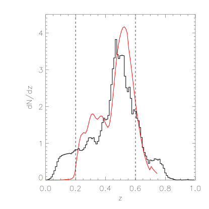
Figure 1: The LRG redshift distribution. The black histogram shows the photo-$z$ distribution, the red curve is the true redshift distribution estimated by regularized deconvolution of the photo-$z$ errors.

III Lensing of CMB

III.1 Definitions

Gravitational lensing re-maps the primordial CMB anisotropy $\tilde{T}$ into a lensed temperature $T$ according to

$$T(\hat{\bf n})=\tilde{T}(\hat{\bf n}+{\bf d}(\hat{\bf n})),$$ (4)

where the 2-vector ${\bf d}$ is the deflection angle of null geodesics. To first order in the metric perturbations, ${\bf d}$ can be expressed as the gradient of a scalar lensing potential, ${\bf d}=\nabla\Phi$, where $\nabla$ is the derivative on the unit (celestial) sphere. We may also define the convergence $\kappa=-{1\over 2}\nabla\cdot{\bf d}$. Assuming the primordial CMB is statistically isotropic with some power spectrum $C_{l}$, it can be shown Hu (2001a); Okamoto and Hu (2003) that the multipole moments of the lensed temperature field have covariance

$$\langle T_{l_{1}m_{1}}^{\ast}T_{l_{2}m_{2}}\rangle = C_{l_{1}}\delta_{l_{1}l_{2}}\delta_{m_{1}m_{2}}+\sum_{LM}(-1)^{m_{2}}{\cal J}_{Ll_{1}l_{2}}$$ (7)

$$\times{\left(\begin{array}[]{ccc}l_{1}&l_{2}&L\\ -m_{1}&m_{2}&-M\end{array}\right)}\kappa_{LM},$$

where we have introduced the Wigner $3j$ symbol, and the coupling coefficient is

$${\cal J}_{Ll_{1}l_{2}} = {2\over L(L+1)}\sqrt{(2L+1)(2l_{1}+1)(2l_{2}+1)\over 16\pi}$$ (10)

$$\times\bigl{\{}[L(L+1)+l_{1}(l_{1}+1)-l_{2}(l_{2}+1)]C_{l_{1}}$$

$$+[L(L+1)-l_{1}(l_{1}+1)+l_{2}(l_{2}+1)]C_{l_{2}}\bigr{\}}$$

$$\times{\left(\begin{array}[]{ccc}l_{1}&l_{2}&L\\ 0&0&0\end{array}\right)}.$$

The WMAP satellite does not directly measure $T$, but rather a beam-convolved temperature:

$$\dot{T}^{\alpha}(\hat{\bf n})=\int B^{\alpha}(\hat{\bf n},\hat{\bf n}^{\prime})T(\hat{\bf n}^{\prime})d^{2}\hat{\bf n}^{\prime}+{\rm noise}.$$ (11)

(Here $\alpha$=K1..W4 are the differencing assemblies.) In most of this analysis we have approximated the beam by the WMAP circularized beam transfer function Page et al. (2003b). The temperature multipole moments recovered assuming a circular beam are

$$\hat{T}^{\alpha}_{lm}=\frac{\dot{T}^{\alpha}_{lm}}{B_{l}^{\alpha}},$$ (12)

where $B_{l}^{\alpha}$ are the beam transfer functions. If the beam is truly circular, Eq. (12) returns an unbiased estimator of the beam-deconvolved CMB temperature; in Sec. VI.3, we will consider the effect of the WMAP beam ellipticity on lensing estimation. Note further that $\hat{T}^{\alpha}_{lm}$ is only well-determined up to some maximum multipole $l$ because the $B_{l}^{\alpha}$ drop to zero at high $l$.

III.2 Theoretical predictions for lensing

In this paper, we aim to measure the galaxy-convergence cross-correlation, $C^{g\kappa}_{l}$, where $g=\delta n/\bar{n}$ is the projected fractional overdensity of galaxies; this section briefly presents the theoretical prediction from the $\Lambda$CDM cosmology. In a spatially flat Friedmann-Robertson-Walker universe described by general relativity, the convergence is given in terms of the fractional density perturbation $\delta$ by:

$$\kappa(\hat{\bf n})=4\pi G_{N}\bar{\rho}_{0}\int\frac{\chi(\chi_{CMB}-\chi)}{\chi_{CMB}}(1+z)\delta(\chi,\hat{\bf n})d\chi,$$ (13)

where $\chi$ is the comoving radial distance, $z$ is the redshift observed at radial distance $\chi$, $\bar{\rho}_{0}$ is the present-day mean density of the universe, and $\chi_{CMB}$ is the comoving distance to the CMB. The galaxy overdensity does not come from a “clean” theoretical prediction, but on large scales it can be approximated by

$$g(\hat{\bf n})=\frac{\int b_{g}{\cal N}(\chi)\delta(\chi,\hat{\bf n})d\chi}{\int{\cal N}(\chi)d\chi},$$ (14)

where ${\cal N}(\chi)$ is the distribution in comoving distance and $b_{g}$ is the galaxy bias. (The SDSS LRG sample is at low redshift $z\leq 0.7$ and does not have a steep luminosity function at the faint end of our sample, so we neglect the magnification bias.) For $l\gg 1$ and smooth power spectra for matter and galaxies, this may be approximated by the Limber integral:

$$C^{g\kappa}_{l} = 4\pi G_{N}\bar{\rho}_{0}$$ (15)

$$\times\frac{\int b_{g}{\cal N}(\chi)({1\over\chi}-{1\over\chi_{CMB}})(1+z)P_{\delta}(\frac{l}{\chi})d\chi}{\int{\cal N}(\chi)d\chi},\;\;\;$$

where the matter power spectrum $P_{\delta}$ is evaluated at comoving wavenumber $k=l/\chi$ and at the redshift corresponding to conformal time $\eta_{0}-\chi$. It is obtained using the transfer functions from CMBFast Seljak and Zaldarriaga (1996) and the best-fit 6-parameter flat $\Lambda$CDM cosmological model from WMAP and SDSS data from Ref. Tegmark et al. (2004) ($\Omega_{b}h^{2}=0.0232$; $\Omega_{m}h^{2}=0.1454$; $h=0.695$; $\tau=0.124$; $\sigma_{8}=0.917$; $n_{s}=0.977$). We have found that varying each of these parameters over their $1\sigma$ uncertainty ranges gives a $\pm 18\%$ effect for $\sigma_{8}$ (for which $C^{g\kappa}_{l}$ scales as $\propto\sigma_{8}^{2}$) and $\pm<14\%$ effect for the other parameters. Since the overall significance of the detection is only 0.9$\sigma$, this dependence of the template $C^{g\kappa}_{l}$ on cosmological parameters will be neglected here.

The lensing signal is on large scales and so we have not used a nonlinear mapping. The peak of the LRG redshift distribution is at $z\sim 0.5$, corresponding to a comoving angular diameter distance $\sim 1.3h^{-1}$ Gpc, in which case the smallest angular scales we use ($l=300$) correspond to $k=0.23h$ Mpc^-1 and $\Delta^{2}(k)=0.7$. The nonlinear evolution at this scale according to the Peacock-Dodds formula Peacock and Dodds (1996) is a $10\%$ correction to the matter power spectrum and is thus much smaller than the error bars presented in this paper (although it is not obvious what this implies about the galaxy-matter cross-spectrum, which is the quantity that should appear in Eq. 15). Future applications of CMB lensing in precision cosmology will of course require accurate treatment of the nonlinear evolution.

In this paper, we will assume that galaxy bias $b_{g}$ is constant so that it may be pulled out of the integrals in Eqs. (14) and (15). If the bias varies with redshift (as suggested by e.g. Fry (1996)), then the best-fit value of $b_{g}$ will be some weighted average of $b_{g}$ over the redshift distribution; this need not be the same weighted average that one observes from the auto-power spectrum, since the latter is weighted differently. Computation of the auto-power in photometric redshift slices Padmanabhan et al. (2004a) suggests that over the redshift range $0.2\leq z\leq 0.6$ the bias varies from $1.7$–$1.9$; this variation can safely be neglected given our current statistical errors. Note however that a detection of $b_{g}\neq 0$ via a fit to Eq. (15) assuming constant $b_{g}$ would rule out $C_{l}^{g\kappa}=0$ and hence would be robust evidence for a galaxy-convergence correlation, regardless of the redshift dependence of the bias.

III.3 Lensing reconstruction

We construct lensing deflection maps using quadratic reconstruction methods Bernardeau (1997); Seljak and Zaldarriaga (1999); Guzik et al. (2000); Zaldarriaga (2000); Hu (2001b); Okamoto and Hu (2002); Hu and Okamoto (2002); Okamoto and Hu (2003); Cooray (2004), which have been shown to be near-optimal for lensing studies of the CMB temperature on large ($l<3500$) scales Hirata and Seljak (2003a). Non-quadratic methods may be superior if CMB polarization is used Hirata and Seljak (2003b), or on very small scales Seljak and Zaldarriaga (2000); Vale et al. (2004); Dodelson (2004); these cases are not of interest for WMAP, since the sensitivity is insufficient to map the CMB polarization and arcminute scales are unresolved. Quadratic estimation takes advantage of the cross-coupling of different multipoles induced by gravitational lensing, namely the $O(\kappa_{LM})$ term in Eq. (7). The maximum signal-to-noise statistic for CMB weak lensing is the divergence of the temperature-weighted gradient. We construct, for each pair of differencing assemblies $\alpha$ and $\beta$, the temperature-weighted gradient vector field $\tilde{\bf G}^{\alpha\beta}$:

$$\tilde{\bf G}^{\alpha\beta}(\hat{\bf n}) = {1\over 2}\biggl{(}[W\hat{T}^{\alpha}](\hat{\bf n})\nabla[CW\hat{T}^{\beta}](\hat{\bf n})$$ (16)

$$+[W\hat{T}^{\beta}](\hat{\bf n})\nabla[CW\hat{T}^{\alpha}](\hat{\bf n})\biggr{)},$$

where $W\hat{T}$ and $CW\hat{T}$ are defined by the convolution relations $[W\hat{T}^{\alpha}]_{lm}=W_{l}\hat{T}^{\alpha}_{lm}$ and $[CW\hat{T}^{\alpha}]_{lm}=C_{l}W_{l}\hat{T}^{\alpha}_{lm}$. Note that Eq. (16) is exactly the same as the $\tilde{\bf G}$ statistic of Ref. Hu (2001b) except that we have multiple differencing assemblies, and we have left open the choice of the weight $W_{l}$. While $W_{l}=(C_{l}+C_{l}^{noise})^{-1}$ is statistically optimal, there are also practical considerations that affect this choice. Specifically, it is desirable that the $W\hat{T}$ and $CW\hat{T}$ convolutions are almost-local functions of the CMB temperature (to minimize leakage from the Galactic Plane), and that the same $W_{l}$ be used for all differencing assemblies (so that any frequency dependence of our results can be attributed to foregrounds or noise, rather than merely a change in which primary CMB modes we are studying). We choose the following weight function:

$$W_{l}=\left[C_{l}+(0.03461\mu{\rm K}^{2})e^{l(l+1)/300^{2}}\right]^{-1},$$ (17)

which clearly has the optimal $C_{l}^{-1}$ dependence in the high signal-to-noise regime. Note that in the range of $l$ we use ($l\leq 800$), the $W_{l}$ drop to zero with increasing $l$ faster than the Q-band beam transfer functions. Hence the computation of $W\hat{T}^{Q1,Q2}$ are stable even though $\hat{T}^{Q1,Q2}$ are beam-deconvolved. Due to their narrower beams, this stability also applies to the V and W-band DAs. The K1 and Ka1 DAs have wider beams and hence lensing reconstruction using the weight Eq. (17) is unstable for these DAs. We set $W_{0}=W_{1}=0$ to reject the monopole (not observed by WMAP) and dipole signals. The power spectrum $C_{l}$ used for the lensing reconstruction is WMAP best-fit $\Lambda$CDM model with scalar spectral running $\alpha_{s}$ Spergel et al. (2003) to the CMB data (WMAP+ACBAR Kuo et al. (2002) +CBI Pearson and Cosmic Background Imager Collaboration (2002)). Errors in the $C_{l}$ used in the lensing reconstruction cannot produce a spurious galaxy-temperature correlation because they result only in a calibration error in the lensing estimator. Furthermore, WMAP has determined the $C_{l}$ to within several percent (except at the low multipoles, which give a subdominant contribution to both $W\hat{T}$ and $\nabla CW\hat{T}$), whereas the lensing cross-correlation signal is only present at the $1\sigma$ level, this error is not important for the present analysis.

In the reconstruction method of Ref. Hu (2001b), a filtered divergence of $\tilde{\bf G}$ is taken to extract the lensing field. We avoid this step because it is highly nonlocal, and hence can smear Galactic plane contamination into the regions of sky used for lensing analysis. In principle, we would prefer to directly cross-correlate $\tilde{\bf G}$ with the LRG map, but this too is difficult because the noise power spectrum of $\tilde{\bf G}$ is extremely blue. We compromise by computing ${\bf v}$, a Gaussian-filtered version of $\tilde{\bf G}$:

$$v_{lm}^{(\parallel,\perp)}=e^{-l(l+1)\sigma_{0}^{2}/2}\tilde{G}_{lm}^{(\parallel,\perp)}.$$ (18)

Here $\parallel$ and $\perp$ represent the longitudinal (vector) and transverse (axial) multipoles, which are the vector analogues of the tensor $E$ and $B$ multipoles. The Gaussian filter eliminates the troublesome high-$l$ power present in $\tilde{\bf G}(\hat{\bf n})$ and makes ${\bf v}$ suitable for cross-correlation studies. We have chosen a width $\sigma_{0}=0.01$ radians (34 arcmin).

The vector field ${\bf v}$ can be written in terms of the temperatures $\hat{T}$ directly in harmonic space. The longitudinal components are given by

$$v_{lm}^{\alpha\beta(\parallel)} = (-1)^{m}\sum_{l^{\prime}l^{\prime\prime}}{\cal K}_{ll^{\prime}l^{\prime\prime}}\sum_{m^{\prime}m^{\prime\prime}}{\left(\begin{array}[]{ccc}l&l^{\prime}&l^{\prime\prime}\\ -m&m^{\prime}&m^{\prime\prime}\end{array}\right)}$$ (22)

$$\times{\hat{T}^{\alpha}_{l^{\prime}m^{\prime}}\hat{T}^{\beta}_{l^{\prime\prime}m^{\prime\prime}}+\hat{T}^{\beta}_{l^{\prime}m^{\prime}}\hat{T}^{\alpha}_{l^{\prime\prime}m^{\prime\prime}}\over 2},$$

where we have defined:

$${\cal K}_{ll^{\prime}l^{\prime\prime}} = {\left(\begin{array}[]{ccc}l&l^{\prime}&l^{\prime\prime}\\ 0&0&0\end{array}\right)}\sqrt{(2l+1)(2l^{\prime}+1)(2l^{\prime\prime}+1)\over 16\pi l(l+1)}$$ (26)

$$\times[l(l+1)-l^{\prime}(l^{\prime}+1)+l^{\prime\prime}(l^{\prime\prime}+1)]C_{l^{\prime\prime}}W_{l^{\prime}}W_{l^{\prime\prime}}$$

$$\times e^{-l(l+1)\sigma_{0}^{2}/2}.$$

We will not need the formula for the transverse components. While we perform the reconstruction (Eqs. 16 and 18) in real space, the harmonic-space relation (Eq. 22) is useful for computing the response of the estimator, and for estimating foreground contamination and beam effects. In particular, from the orthonormality relations for Wigner $3j$-symbols, we have

$$\langle v^{\alpha\beta(\parallel)}_{lm}\rangle=\sum_{l^{\prime}l^{\prime\prime}}{{\cal J}_{ll^{\prime}l^{\prime\prime}}{\cal K}_{ll^{\prime}l^{\prime\prime}}\over 2l+1}\kappa_{lm}\equiv R_{l}\kappa_{lm},$$ (27)

which defines the calibration of ${\bf v}$ as an estimator of the lensing field. The response factor $R_{l}$ is shown in Fig. 2; we have verified this response factor in simulations (Sec. IV.3).

Figure 2: The response factor $R_{l}$ of Eq. (27) satisfying $\langle v^{\alpha\beta(\parallel)}_{lm}\rangle=R_{l}\kappa_{lm}$.

There are 36 pairs of differencing assemblies that could be used to produce estimated lensing maps ${\bf v}^{\alpha\beta}_{lm}$: the 8 “autocorrelations” ($\alpha=\beta$) and 28 “cross-correlations” ($\alpha\neq\beta$). Note that instrument noise that is non-uniform across the sky can produce a bias in the “autocorrelation”-derived lensing map ${\bf v}^{\alpha\alpha}$. In principle the noise bias could be estimated and subtracted, just as can be done for the power spectrum. However, this is dangerous if the noise properties are not very well modeled. Since the WMAP noise is in fact strongly variable across the sky we only use the “cross-correlation” $\alpha\neq\beta$ maps.

One problem that we find with this method is that the ${\bf v}$ field contains “ghosts” caused by the Galactic plane (where small-scale temperature fluctuations of several millikelvin or more can occur due to Galactic emission). We solve this problem by setting $T=0$ within the WMAP Kp4 Bennett et al. (2003c) Galactic plane mask. We have verified that using the Kp2 mask instead produces only small changes to the results.

The weight functions $W_{l}$ and $C_{l}W_{l}$ are shown in Fig. 3. We also show the real-space weights, given by

$$W(\theta)=\sum_{l}{2l+1\over 4\pi}W_{l}P_{l}(\cos\theta),$$ (28)

and similarly for $[CW](\theta)$.

Figure 3: (a) The weight functions $W_{l}$ and $C_{l}W_{l}$. (b) The same weight functions in real-space (Eq. 28); $W\hat{T}$ and $CW\hat{T}$ are obtained by convolving the (beam-deconvolved) temperature $\hat{T}$ with these kernels.

III.4 Frequency-averaged lensing maps

The methodology outlined in Sec. III.3 allows us to construct 28 lensing maps ${\bf v}^{\alpha\beta}$ corresponding to the 28 pairs of differencing assemblies. For this analysis, we need to produce an “averaged” lensing map ${\bf v}^{(TT)}$ based on a minimum-variance linear combination of the 28 DA-pair maps. The averaged lensing map is determined by the weights $a^{(TT)}_{\alpha\beta}$:

$${\bf v}^{(TT)}=\sum_{\alpha\beta}a^{(TT)}_{\alpha\beta}{\bf v}^{\alpha\beta}.$$ (29)

We select these weights to minimize the amount of power in ${\bf v}^{(TT)}$, subject to the restriction $\sum a^{(TT)}_{\alpha\beta}=1$; this is done by minimizing the total vector power in ${\bf v}$ between multipoles 50 and 125: ${\cal P}=\sum_{l=50}^{125}\sum_{m=-l}^{l}|v^{(TT)\,\parallel}_{lm}|^{2}$, which is a quadratic function of the weights $a^{(TT)}_{\alpha\beta}$. The optimal weights $a^{(TT)}_{\alpha\beta}$ are complicated to establish analytically since the maps ${\bf v}^{\alpha\beta}$ are highly correlated. We have therefore minimized ${\cal P}$ using a simulated lensing map (see Sec. IV.3). Using a simulated map rather than the real data avoids the undesirable possibility of the weights being statistically correlated with the data. We also fix $a^{(TT)}_{Q1,Q2}=0$ because the ${\bf v}^{Q1,Q2}$ map would be the most heavily contaminated by point sources. The weights so obtained are shown in Table 1. A map of $\nabla\cdot{\bf v}^{(TT)}$, smoothed to 30 arcmin resolution (Gaussian FWHM) is shown in Fig. 4.

Figure 4: The divergence of the lensing vector field map, $\nabla\cdot{\bf v}^{(TT)}$, smoothed with a 30 arcmin FWHM Gaussian, and displayed in Galactic Molleweide projection. Note the prominent artifacts surrounding the Galactic plane cut and the point sources (which are removed by the Kp05$\cap$S10$\setminus$ps₂ cut).

Also, to study foreground effects on lensing estimation, we would like to construct averaged lensing maps ${\bf v}^{(QQ)}$, ${\bf v}^{(QV)}$, etc. where we only average over differencing assemblies at the same frequency, thereby preserving frequency-dependent information. There are six of these maps (QQ, QV, QW, VV, VW, and WW); the last column of Table 1 shows the weights used to construct them.

Table 1: The weights $a_{\alpha\beta}$ used for the overall-averaged lensing map $a^{(TT)}_{\alpha\beta}$, and the six “individual frequency” maps $a^{(QQ)}_{\alpha\beta},...,a^{(WW)}_{\alpha\beta}$.

DA pair ($\alpha\beta$)		$a^{(TT)}_{\alpha\beta}\!\!\!\!\!\!\!\!$		$a^{(\nu_{1}\nu_{2})}_{\alpha\beta}\!\!\!\!\!\!\!\!$
Q1,Q2		$0.000000$		$1.000000$
Q1,V1		$0.063759$		$0.220605$
Q1,V2		$0.075370$		$0.267859$
Q2,V1		$0.061538$		$0.227341$
Q2,V2		$0.098884$		$0.284196$
Q1,W1		$0.031583$		$0.167730$
Q1,W2		$0.026896$		$0.113943$
Q1,W3		$0.018391$		$0.094086$
Q1,W4		$0.028571$		$0.130429$
Q2,W1		$0.023816$		$0.158925$
Q2,W2		$0.017153$		$0.107379$
Q2,W3		$0.014494$		$0.097062$
Q2,W4		$0.027164$		$0.130444$
V1,V2		$0.106330$		$1.000000$
V1,W1		$0.053278$		$0.150880$
V1,W2		$0.029381$		$0.094494$
V1,W3		$0.029664$		$0.087425$
V1,W4		$0.035463$		$0.107193$
V2,W1		$0.048598$		$0.168035$
V2,W2		$0.049979$		$0.137365$
V2,W3		$0.034621$		$0.115438$
V2,W4		$0.046029$		$0.139169$
W1,W2		$0.016453$		$0.199003$
W1,W3		$0.014448$		$0.170408$
W1,W4		$0.019908$		$0.232958$
W2,W3		$0.014514$		$0.129381$
W2,W4		$0.003365$		$0.133767$
W3,W4		$0.010347$		$0.134484$

The power spectrum of the longitudinal mode of ${\bf v}$ obtained on the cut sky (Kp05$\cap$S10$\setminus$ps₂ cut, which excludes point sources; see Sec. IV.1) is shown in Fig. 5.

Figure 5: The longitudinal mode power spectrum $C_{l,\parallel}^{vv}$ within the Kp05$\cap$S10$\setminus$ps₂ cut (solid line), for each of the six frequency pairs. The points show 10 simulations (containing no lensing or foregrounds). Since the purpose of this plot is to compare the simulations to the actual data, the sky cut has not been deconvolved, rather we have plotted the average of $|\int{\bf v}\cdot{\bf Y}^{(\parallel)\ast}_{lm}d^{2}\hat{\bf n}/f_{sky}|^{2}$ within bands of width $\Delta l=10$.

IV Cross-correlation computation

IV.1 Sky cuts

In some regions of the sky, particularly the Galactic plane, microwave emission from within the Milky Way and from nearby galaxies dominates over the cosmological signal. For their CMB analysis, the WMAP team removed this signal by (i) masking out a region based on a smoothed contour of the K-band temperature, which they denote “Kp2” Bennett et al. (2003c), and (ii) projecting out of their map microwave emission templates for synchrotron, free-free, and dust emission based on other observations Haslam et al. (1981, 1982); Finkbeiner (2003a); Schlegel et al. (1998); Finkbeiner et al. (1999). Template projection is dangerous for cross-correlation studies involving galaxies because the dust template of Ref. Schlegel et al. (1998) is used to extinction-correct the LRG magnitudes, thus template errors could introduce spurious correlations between the CMB and galaxy maps. Since visual inspection of the uncleaned WMAP maps reveals Galactic contamination outside the Kp2-rejected region at all five frequencies, we have used the more conservative Kp0 mask in Sec. VI.4 for our galaxy-temperature correlations. Because the SDSS covers only a small portion of the sky, we speed up the cross-correlation computation by using only WMAP data in the vicinity of the SDSS survey region. We define the “S10” region to consist of those pixels within 10 degrees of the SDSS survey area. The Kp0$\cap$S10 cut accepts 774,534 HEALPix pixels (10,157 sq. deg.).

When analyzing primary CMB anisotropies, it is customary to mask detected point sources in order to eliminate this spurious contribution to the temperature. For secondary anisotropy studies, the analysis should be done both with and without the point sources because the point sources may correlate with large scale structure, hence naively masking them could lead to misleading results. Therefore for the galaxy-temperature correlation used in Sec. VI.4 we have constructed the Kp0$\cap$S10$\setminus$ps mask by rejecting all pixels within the WMAP point source mask (with a 0.6 degree exclusion radius around each source). The Kp0$\cap$S10$\setminus$ps cut accepts 756,078 HEALPix pixels (9915 sq. deg.).

For the lensing analysis, we must use a more conservative mask than Kp0 because the lensing estimator ${\bf v}$ is a nonlocal function of the CMB temperature, hence ${\bf v}(\hat{\bf n})$ responds to foreground emission several degrees away from $\hat{\bf n}$. We have therefore constructed a “Kp05” mask consisting of all pixels within Kp0 that are at least 5 degrees away from the Kp0 boundary; the Kp05$\cap$S10 mask used for the lensing analysis accepts 753,242 HEALPix pixels (9,878 sq. deg.). We have also constructed a point source-removed version, Kp05$\cap$S10$\setminus$ps₂ , in which all pixels within 2 degrees of the point sources are rejected. This mask accepts 598,795 HEALPix pixels (7,853 sq. deg.).

IV.2 Galaxy-convergence correlation

Having constructed the vector field ${\bf v}$, we proceed to compute its cross-correlation $C^{gv}_{l}$ with the LRG map. We construct the data vector

$${\bf x}^{T}=({\bf x}^{T}_{LRG},{\bf x}^{T}_{lens})$$ (30)

of length $N_{pix}^{(LRG)}+2N_{pix}^{(CMB)}$, where ${\bf x}_{LRG}$ is a vector containing the galaxy overdensities $g=\delta n/\bar{n}$ in each SDSS pixel, and ${\bf x}_{lens}$ consists of the two components of ${\bf v}$ at each WMAP pixel. (We will suppress the frequency indices $(QQ)$, $(QV)$, etc. on ${\bf v}$ for clarity; it is understood that the analysis below is repeated for each pair of frequencies.) The covariance of ${\bf x}$ is then:

$${\sf C}\equiv\langle{\bf xx}^{T}\rangle=\left(\begin{array}[]{cc}{\sf C}^{(LRG)}&{\sf C}^{(\times)}\\ {\sf C}^{(\times)T}&{\sf C}^{(lens)}\end{array}\right).$$ (31)

The cross-correlation matrix ${\sf C}^{(\times)}$ has components:

$$C^{(\times)}_{i,jK}=\sum_{lm}C_{l}^{gv}Y_{lm}^{\ast}(\hat{\bf n}_{i}){\bf Y}_{lm}^{\parallel}(\hat{\bf n}_{j})\cdot\hat{\bf e}_{K},$$ (32)

where $i$ represents an SDSS pixel index, $j$ is a WMAP pixel index, and $K=\hat{\theta},\hat{\phi}$ indicates which component of the vector ${\bf v}$ is under consideration. We bin the cross-spectrum $C_{l}^{gv}$ into bands,

$$C_{l}^{gv}=\sum_{A}c^{A}\left\{\begin{array}[]{lcl}1&&l_{\rm min}(A)\leq l<l_{\rm max}(A)\\ 0&&{\rm otherwise}\end{array}\right.,$$ (33)

and take the $c^{A}$ as the parameters to be estimated.

In order to construct an optimal estimator for the galaxy-convergence cross-spectrum, we need a prior auto-correlation matrix for the LRGs and for the lensing map. (This is a “prior” in the sense of quadratic estimation theory Hamilton (1997a, b); Tegmark (1997); Padmanabhan et al. (2003), and has nothing to do with Bayesian priors.) We take a prior of the form

$${\sf C}^{(LRG)}_{ij}=\sum_{lm}C_{l}^{gg}Y_{lm}^{\ast}(\hat{\bf n}_{i})Y_{lm}(\hat{\bf n}_{j})+N\delta_{ij},$$ (34)

where $C_{l}^{gg}$ is the galaxy power spectrum (excluding Poisson noise) and $N$ is the noise variance per pixel. We have taken $N$ to be the reciprocal of the mean number of galaxies per pixel, appropriate for Poisson noise (we use the mean galaxy density per pixel to avoid biases associated with preferential weighting of pixels containing fewer galaxies). The prior power spectrum $C_{l}^{(LRG)}$ is determined by application of a pseudo-$C_{l}$ estimator to the LRG maps; the resulting power spectrum is shown in Fig. 6. We have set $C_{l}^{gg}=0.01\gg C_{l\geq 2}^{gg}$ for $l=0,1$ to reject the galaxy monopole (“integral constraint”) and dipole modes from the cross-correlation analysis.

Figure 6: The prior power spectrum used for the LRG map, obtained by application of a pseudo-$C_{l}$ estimator to the SDSS scan region. The dashed line shows the Poisson noise.

It can be shown Hamilton (1997a, b); Tegmark (1997) that for Gaussian data with small ${\sf C}^{(\times)}$, the optimal estimator for the $c^{A}$ would be obtained by taking the unbiased linear combinations of the ${\bf x}_{LRG}^{T}{\sf C}^{(LRG)-1}{\sf P}_{A}{\sf C}^{(lens)-1}{\bf x}_{lens}$. These estimators are frequently called “QML” or quadratic maximum-likelihood estimators, although they are, strictly speaking, not maximum-likelihood. We do not have the full matrix ${\sf C}^{(lens)}$, and our only knowledge of this matrix comes from simulations. Thus we have instead constructed, for each lensing map ${\bf v}^{\alpha\beta}$, the quadratic combinations:

$$Q_{A}={\bf x}^{T}_{LRG}{\sf C}^{(LRG)\,-1}{\partial{\sf C}^{(\times)}\over\partial c^{A}}{\bf x}_{lens},$$ (35)

where $A$ represents a band index. This differs from the QML estimators in that the ${\sf C}^{-1}$ weighting is applied only to the LRGs, while uniform weighting is applied to the CMB lensing map ${\bf v}$; thus Eq. (35) can be viewed as a sort of half-QML, half-pseudo-$C_{l}$ estimator for the cross-spectrum. The expectation value of $Q_{A}$ can be determined from Eq. (31); it is:

$$\langle Q_{A}\rangle={\rm~{}Tr~{}}\left[{\partial{\sf C}^{(\times)T}\over\partial c^{B}}{\sf C}^{(LRG)\,-1}{\partial{\sf C}^{(\times)}\over\partial c^{A}}\right]c^{B}\equiv R_{AB}c^{B},$$ (36)

which defines the response matrix $R_{AB}$. Note that unlike the response matrix of the optimal quadratic estimator, $R_{AB}$ is not equal to the Fisher matrix. The trace in Eq. (36) may be computed using a stochastic-trace algorithm:

$$R_{AB}=\langle({\sf C}^{(LRG)\,-1}{\bf y})^{T}{\partial{\sf C}^{(\times)}\over\partial c^{A}}{\partial{\sf C}^{(\times)T}\over\partial c^{B}}{\bf y}\rangle,$$ (37)

where ${\bf y}$ is a random vector of length $N_{pix}^{(LRG)}$ consisting of $\pm 1$ entries. The vectors in Eqs. (35) and (37) are constructed in pixel space. Harmonic space is used only as an intermediate step in the convolutions required to compute the matrix-vector multiplications, e.g. ${\partial{\sf C}^{(\times)T}\over\partial c^{B}}{\bf y}$; these are computed by the usual method of converting to harmonic space, multiplying by $\partial C_{l}^{gv}/\partial c^{B}$, and converting back to real space. The matrix inverse operations are performed iteratively as described in Appendix B. This method allows us to easily compute estimators for the band cross-powers,

$$\hat{c}^{A}=[R^{-1}]^{AB}Q_{B}.$$ (38)

While this estimator is manifestly unbiased, we do not know its uncertainty because we do not know the covariance ${\sf C}^{(lens)}$ of the ${\bf v}$-field. We determine the uncertainty via a Monte Carlo method: we construct random CMB realizations according to the null hypothesis of no lensing in all eight DAs used for the lensing reconstruction, and feed them through the lensing reconstruction pipeline (Sec. III.3).

In order to estimate the galaxy bias from the binned cross-power spectrum estimators $\hat{c}^{A}$, we need to know the response of each estimator $\hat{c}^{A}$ to the galaxy bias, $d\langle\hat{c}^{A}\rangle/db_{g}$. This is given by

$${d\langle\hat{c}^{A}\rangle\over db_{g}}=[R^{-1}]^{AB}{\rm~{}Tr~{}}\left[{d{\sf C}^{(\times)T}\over db_{g}}{\sf C}^{(LRG)-1}{\partial{\sf C}^{(\times)}\over\partial c^{B}}\right],$$ (39)

which is computed by a stochastic-trace algorithm analogous to Eq. (37). The galaxy-${\bf v}$ correlation matrix $d{\sf C}^{(\times)T}/db_{g}$ is

$${dC^{(\times)}_{i,jK}\over db_{g}}=\sum_{lm}R_{l}{dC^{g\kappa}\over db_{g}}Y_{lm}^{\ast}(\hat{\bf n}_{i}){\bf Y}^{\parallel}_{lm}(\hat{\bf n}_{j})\cdot\hat{\bf e}_{K},$$ (40)

where $R_{l}$ is the lensing response factor of Eq. (27). If we knew $C^{\bf vv}$, it would be optimal to use $C^{{\bf vv}\,-1}$ weighting, in which case we could simply use $d{\sf C}^{(\times)T}/db_{g}$ as a cross-power template with no loss of information. However since we have not calculated $C^{\bf v\bf v}$, and our only information on this covariance matrix comes from the ability to generate random realizations of ${\bf v}$, we cannot do this.

IV.3 Simulations

Simulating lensed and unlensed CMB maps is necessary both for verifying the analysis pipeline as well as for determining the optimal weighting of Sec. III.4. The general procedure used here is to generate a simulated primary CMB temperature $T_{lm}$, convergence $\kappa_{lm}$, and galaxy density fluctuation $\delta n_{lm}$ in harmonic space. These are Gaussian random fields and hence it is a straightforward matter to produce random realizations from the power spectra and cross-spectra of $T$, $\kappa$, and $\delta n$. After generation of the realization, the primary temperature and deflection field (generated from the convergence, assuming an irrotational deflection field) are pixelized in HEALPix resolution 10 (12,582,912 pixels of solid angle $11.8$ arcmin² each). The lensed CMB temperature $\tilde{T}$ is then computed in real space from Eq. (4). Because the “deflected” HEALPix pixels no longer lie on curves of constant latitude, we use a non-isolatitude spherical harmonic transform (see Appendix A; we have used parameters $L^{\prime}=6144$ and $K=11$ since high accuracy is required) to evaluate Eq. (4). The beam convolution relevant to each DA is then applied by converting to harmonic space, multiplying by $B_{l}^{\alpha}$ and the pixel window function, and converting back to real space. Finally the simulated CMB temperature field $\dot{T}(\hat{\bf n})$ is degraded to HEALPix resolution 9, and appropriate Gaussian “instrument” noise is added independently to each pixel. Note that the resolution 10 pixels are used here to improve the fidelity of the simulation, in particular to ensure that the effects of the elongated HEALPix pixels on the lensing estimator are properly simulated.

A crude model for the WMAP beam ellipticity is incorporated into the simulations as follows. At each point, we have

$$\dot{T}^{\alpha}(\hat{\bf n})={1\over 2}\sum_{{\rm side}=A,B}\sum_{lm\mu}B_{l\mu}T_{lm}Y_{lm}^{\mu}(\hat{\bf n})\langle e^{i\mu\psi}\rangle,$$ (41)

where the $Y_{lm}^{\mu}$ are spin-weighted spherical harmonics and the beam moments $B_{l\mu}$ are the multipole moments of the beam in instrument-fixed coordinates (with the “North Pole” along the boresight and the $\phi^{\prime}=0$ meridian in the scan direction):

$$B_{l\mu}=\sqrt{4\pi\over 2l+1}\int_{4\pi}B(\hat{\bf n}_{inst})Y_{l\mu}^{\ast}(\hat{\bf n}_{inst})d^{2}\hat{\bf n}_{inst}.$$ (42)

The average value $\langle e^{i\mu\psi}\rangle$ is taken over the position angles of the instrument when $\hat{\bf n}$ is scanned. The sum over sides is over the two sides of WMAP. Equation (41) is only an approximation because (i) the two sides of the differencing assembly may not scan each pixel exactly the same number of times, or may have slightly different weights; and (ii) because WMAP is a differential instrument, $\langle\dot{T}^{\alpha}(\theta,\phi)\rangle$ is also affected by beam-ellipticity effects on other parts of the sky. Since the two beams of a given DA are separated by $\sim 140$ degrees, this results in an “echo” of a given microwave source at a separation of 140 degrees Hinshaw et al. (2003b) (and higher-order echoes should also be present); we have neglected these.

We have made several further approximations to Eq. (41) in order to speed up the simulations. First, we have only included the ellipticity modes $\mu=\pm 2$, since these dominate the difference between the azimuthally symmetrized beam and the true beam. The beam ellipticity is thus described by the real and imaginary parts of $B_{l,2}$; recall $B_{l,-2}=B_{l,2}^{\ast}$. We have calculated $B_{l,2}$ by taking the non-isolatitude spherical harmonic transform of the WMAP beam maps Page et al. (2003b). Secondly, because the side $A$ and $B$ beams are approximate mirror-images of each other, we have only considered the component of the beam ellipticity along the scan direction. The component of the beam ellipticity at 45 degrees to the scan direction is suppressed because, to the extent that the side $A$ and $B$ beams are mirror images and scan each pixel the same number of times, this component cancels in Eq. 41 when we sum over the two sides.

Finally, we have used a simple model for the scan pattern $\langle e^{i\mu\psi}\rangle$ for each DA. The WMAP scan pattern is crudely approximated as a rotation around the spacecraft $-Z$ axis, followed by a precession of this axis in a 22.5 degree radius circle around the anti-Sun point, followed by rotation of the anti-Sun point along the ecliptic plane. Relative to the spacecraft $-Z$ axis, the effective number of observations in one rotation is: $N_{obs}(\theta,\phi)=-N_{obs}\langle e^{2i\psi}\rangle=K\delta(\cos\theta-\cos\theta_{c})/2\pi$, where $\theta_{c}$ is the angle between the instrument boresight and the spacecraft $-Z$ axis, and $K$ is a constant. We can convert these to harmonic space in the spacecraft coordinates,

$$[N_{obs}]_{lm}(-Z) = K\delta_{m0}Y_{l0}(\theta_{c},0);$$

$$\left[N_{obs}\langle e^{2i\psi}\rangle\right]_{lm}(-Z) = -K\delta_{m0}Y^{2}_{l0}(\theta_{c},0).$$ (43)

Averaged over the precession cycle of WMAP, this becomes

$$[N_{obs}]_{l0}({\rm av}) = KP_{l}(\cos 22.5{\rm~{}deg})P_{l}(0)Y_{l0}(\theta_{c},0);$$

$$\left[N_{obs}\langle e^{2i\psi}\rangle\right]_{l0}({\rm av}) = -KP_{l}(\cos 22.5{\rm~{}deg})$$ (44)

$$\times P_{l}(0)Y_{l0}^{2}(\theta_{c},0).$$

(The $m\neq 0$ moments vanish.) Once these have been obtained, we may transform back to real space and find $\langle e^{2i\psi}\rangle$ by division. This is then rotated from the ecliptic to the Galactic coordinate system. To speed up computation, the elliptical correction to the beam was only computed on the HEALPix resolution 9 grid whereas the dominant circular part was computed on the resolution 10 grid and then degraded by pixel-averaging.

V Results

V.1 Galaxy-convergence cross-spectrum

The individual cross-spectra obtained at different frequencies are shown in Fig. 7. The frequency-averaged cross-spectrum is shown in Fig. 8, both with and without point sources.

Figure 7: The galaxy-convergence correlation using the Kp05$\cap$S10$\setminus$ps₂ cut, for each of the six combinations of frequencies. The error bars are strongly correlated across different frequencies. The dashed curve shows the theoretical signal for our best-fit value of $b_{g}=1.81$.

Figure 8: The galaxy-convergence correlation, using the frequency-averaged ${\bf v}^{(TT)}$ map. The top panel shows the correlation using the Kp05$\cap$S10$\setminus$ps₂ mask (which rejects point sources). The middle panel shows the correlation using the Kp05$\cap$S10 mask, which does not reject point sources. The bottom panel shows the correlation with the ${\bf v}^{(TT)}$ field rotated by 90 degrees; this should be zero in the absence of systematics (see Sec. VI.1). The error bars are from simulations as described in Sec. V.2. The dashed curve shows the theoretical signal for $b_{g}=1.81$.

V.2 Amplitude determination

We estimate the bias amplitude $b_{g}$ by fitting the observed galaxy-convergence cross-spectrum $C^{g\kappa}_{l}$ to the theoretical model, Eq. (15). We begin by obtaining the covariance matrix $\hat{\Gamma}$ of $\hat{c}^{A}$ as determined from $M=50$ simulations:

$$\hat{\Gamma}^{AB}={1\over M-1}\sum_{i=1}^{M}(\hat{c}^{A}_{i}-\bar{c}^{A})(\hat{c}^{B}_{i}-\bar{c}^{B}).$$ (45)

(The simulated $\hat{c}^{A}$ are generated by producing a random realization of the CMB as described in Sec. IV.3 with no lensing, feeding it through the lensing pipeline, and correlating it against the real SDSS LRG map.) The bias is estimated from the weighted average of the observed cross-powers in our $N=14$ bands:

$$\hat{b}_{g}=\frac{\sum_{A=1}^{N}\hat{c}^{A}{dc^{A}_{th}\over db_{g}}/\hat{\Gamma}^{AA}}{\sum_{A=1}^{N}\left({dc^{A}_{th}\over db_{g}}\right)^{2}/\hat{\Gamma}^{AA}},$$ (46)

where $c^{A}_{th}$ is the theoretical prediction for the binned cross-spectrum, Eq. (33); this is directly proportional to the bias, $c^{A}_{th}\propto b_{g}$. The response $dc^{A}_{th}/db_{g}$ is obtained from Eq. (39). It is trivially seen that Eq. (46) is an unbiased estimator of $b_{g}$, regardless of the covariance of the $\hat{c}^{A}$. Since we are working in harmonic space with bands of width $\Delta l\geq 20>\Delta\theta^{-1}$, where $\Delta\theta$ is the typical width of the survey region (in radians), the different $l$-bands are very weakly correlated, so we have not attempted to further optimize the relative weights of the various cross-power estimators $\hat{c}^{A}$.

The most obvious way to estimate the uncertainty in $\hat{b}_{g}$ by noting that Eq. (46) is a linear function of the $c^{A}$, and substituting in the covariance matrix $\hat{\Gamma}^{AB}$ of the $\{c^{A}\}$:

$$\sigma(\hat{b}_{g};{\rm~{}incorrect})=\frac{\sum_{A,B=1}^{N}\hat{\Gamma}^{AB}{dc^{A}_{th}\over db_{g}}{dc^{B}_{th}\over db_{g}}/\hat{\Gamma}^{AA}\hat{\Gamma}^{BB}}{\left[\sum_{A=1}^{N}\left({dc^{A}_{th}\over db_{g}}\right)^{2}/\hat{\Gamma}^{AA}\right]^{2}}.$$ (47)

This calculation is incorrect for finite number $M<\infty$ of simulations because it neglects the fact that the $\hat{\Gamma}^{AB}$ are themselves random variables. One approach to the problem is to take a sufficiently large number of simulations $M$ that the error in Eq. (47) becomes negligible. The difficulties in this approach are that it could be very computationally intensive; we do not know whether $M$ simulations are “enough” unless we try even larger values of $M$ to check convergence. An alternative method, which we have used here, is to run an additional $M^{\prime}=50$ simulated realizations of $\{\hat{c}^{A}\}$ (identical to those used to compute $\hat{\Gamma}^{AB}$ except for the random number generator seed), compute the bias $\hat{b}_{g}$ from them, and then compute their sample variance. The resulting error bars can be analyzed using the well-known Student’s $t$-distribution. The “$1\sigma$” $t$ error bars (which have 49 degrees of freedom) obtained by this method are shown in Table 2. The mean bias values obtained from these 50 random realizations are shown in the “random” column in the table. Also shown in Table 2 (in the “foreground” columns) are the results obtained by feeding the Galactic foreground templates of Sec. VI.5.2 through the lensing pipeline and correlating these with the real LRG map.

In the case of the Kp05$\cap$S10 cut (last column in Table 2), which does not reject point sources, the ${\bf v}^{(QQ)}$, ${\bf v}^{(QV)}$, and ${\bf v}^{(QW)}$ maps have power spectra that are boosted significantly by point source contamination (see Sec. VI.4.1). Therefore, even if the correlation of the point sources with the galaxies can be neglected, the error $\sigma(b_{g})$ obtained in these bands for the Kp05$\cap$S10 mask is probably underestimated, as noted in the table.

Table 2: The bias $b_{g}$ estimated using several frequency ranges (first column). The second column gives the bias $b_{g}$ obtained with the point sources removed (Kp05$\cap$S10$\setminus$ps₂ cut); these are the numbers that should be thought of as our “result.” The uncertainties are $1\sigma$ with $t$ errors (49 d.o.f.); the first error given used the elliptical beam simulations, the error in parentheses is obtained from circular beam simulations (Sec. VI.3). The “TT” frequency combination is a weighted average of QV, QW, VV, VW, and WW. The column labeled “foreground” show the bias $b_{g}$ obtained by correlating the ${\bf v}$ maps derived from the Galactic foreground maps of Sec. VI.5.2 against the LRG map. Similarly, the column labeled “random” show the bias $b_{g}$ obtained using the average of the 50 random realizations of ${\bf v}$ in place of the WMAP-derived ${\bf v}$ map. The column labeled “TT weight” shows the bias determined by using the same weights as a function of $l$ as for the TT frequency combination in Eq. (46); of course this has no effect on $b_{g}(TT)$. The final column, labeled “Kp05$\cap$S10 ”, is the bias obtained without the point source cut.

Frequency	Bias, $b_{g}$		foreground		random		TT weight		$b_{g}$, Kp05$\cap$S10
QQ	$+3.62\pm 4.48(\pm 4.33)\!\!\!\!\!\!\!\!\!\!\!\!\!\!\!\!\!\!\!\!$		$-0.001640$		$-0.34\pm 0.63$		$+3.13\pm 4.55$		$+6.30\pm 3.93$
QV	$+3.10\pm 2.19(\pm 2.00)\!\!\!\!\!\!\!\!\!\!\!\!\!\!\!\!\!\!\!\!$		$-0.000001$		$+0.07\pm 0.31$		$+3.39\pm 2.29$		$+3.93\pm 1.99$
QW	$-0.11\pm 2.53(\pm 2.35)\!\!\!\!\!\!\!\!\!\!\!\!\!\!\!\!\!\!\!\!$		$-0.000480$		$+0.06\pm 0.36$		$-0.20\pm 2.56$		$+0.48\pm 2.43$
VV	$-1.41\pm 2.95(\pm 3.13)\!\!\!\!\!\!\!\!\!\!\!\!\!\!\!\!\!\!\!\!$		$-0.000737$		$+0.88\pm 0.42$		$+0.34\pm 3.04$		$+0.58\pm 2.35$
VW	$+2.63\pm 2.56(\pm 2.11)\!\!\!\!\!\!\!\!\!\!\!\!\!\!\!\!\!\!\!\!$		$-0.000617$		$+0.35\pm 0.36$		$+2.58\pm 2.62$		$+2.51\pm 2.03$
WW	$+0.23\pm 3.11(\pm 2.71)\!\!\!\!\!\!\!\!\!\!\!\!\!\!\!\!\!\!\!\!$		$-0.000817$		$+0.20\pm 0.44$		$+0.65\pm 3.22$		$-0.75\pm 2.63$
TT	$+1.81\pm 1.92(\pm 1.72)\!\!\!\!\!\!\!\!\!\!\!\!\!\!\!\!\!\!\!\!$		$-0.000449$		$+0.23\pm 0.27$		$+1.81\pm 1.92$		$+2.43\pm 1.58$

The $\hat{\chi}^{2}$ values for fits to zero signal are shown in Table 3. These are obtained using the 14 band cross-power spectra (Fig. 8), and the $14\times 14$ covariance matrix is obtained from 100 simulations,

$$\hat{\chi}^{2}=[\hat{\Gamma}^{-1}(100{\rm~{}sims})]_{AB}c^{A}c^{B}.$$ (48)

Because the number of simulations is finite, there remains some noise in this covariance matrix and this must be taken into account in interpreting the $\hat{\chi}^{2}$. In particular, the $\hat{\chi}^{2}$ variable does not exactly follow the standard $\chi^{2}$ (so we have denoted it with a hat). The distribution and $p$-values can, however be calculated as described in Ref. Hirata et al. (2004), Appendix D. As noted previously, the errors for the Kp05$\cap$S10$\setminus$ps₂ mask in the QQ, QV, and QW combinations are suspect.

Table 3: The $\hat{\chi}^{2}$ values obtained for fits to zero signal from the galaxy-convergence cross-spectrum. The first column shows the results with the Kp05$\cap$S10 mask; the second using the Kp05$\cap$S10$\setminus$ps₂ mask; and the third using the Kp05$\cap$S10$\setminus$ps₂ mask with 90 degree rotation of ${\bf v}$. The $\chi^{2}$ has 14 degrees of freedom (the 14 $l$-bins shown in Fig. 8) and the covariance matrices were obtained from the 100 simulations described in Sec. V.2. As described in the text, the finite number of simulations means that the expectation value of the $\hat{\chi}^{2}$ is not 14 but is larger due to uncertainty in the covariance matrix; the mean of the $\hat{\chi}^{2}$ distribution is 16.5 and the standard deviation is 6.8. We have also given the cumulative probability distributions.

Freq.		Kp05$\cap$S10			Kp05$\cap$S10$\setminus$ps2			Kp05$\cap$S10$\setminus$ps2
								+90 degrees
		$\hat{\chi}^{2}$	$P(<\hat{\chi}^{2})\!\!\!\!\!\!\!\!\!\!$		$\hat{\chi}^{2}$	$P(<\hat{\chi}^{2})\!\!\!\!\!\!\!\!\!\!\!\!$		$\hat{\chi}^{2}$	$P(<\hat{\chi}^{2})\!\!\!\!\!\!\!\!\!\!\!\!$
QQ		51.51	$\!\!\!\!\!\!\!\!\!\!0.9996\!\!\!\!\!\!\!\!\!\!$		16.24	$0.55$		28.24	$0.940$
QV		37.01	$\!\!\!\!\!\!\!\!\!\!0.990\!\!\!\!\!\!\!\!\!\!$		27.51	$0.931$		21.89	$0.81$
QW		16.74	$\!\!\!\!\!\!\!\!\!\!0.58\!\!\!\!\!\!\!\!\!\!$		11.74	$0.26$		21.58	$0.80$
VV		19.08	$\!\!\!\!\!\!\!\!\!\!0.70\!\!\!\!\!\!\!\!\!\!$		11.86	$0.27$		24.85	$0.89$
VW		25.30	$\!\!\!\!\!\!\!\!\!\!0.90\!\!\!\!\!\!\!\!\!\!$		20.28	$0.75$		20.06	$0.74$
WW		11.54	$\!\!\!\!\!\!\!\!\!\!0.25\!\!\!\!\!\!\!\!\!\!$		11.36	$0.24$		21.82	$0.81$
TT		26.90	$\!\!\!\!\!\!\!\!\!\!0.922\!\!\!\!\!\!\!\!\!\!$		19.97	$0.74$		30.71	$0.963$

VI Systematic errors

VI.1 Ninety-degree rotation test

One of the standard systematics tests in weak lensing studies using galaxies as sources has been to rotate all of the galaxies by 45 degrees and look for a shear signal. The 45 degree rotation is used because it interconverts $E$ and $B$ modes, and in the absence of systematics there should be no $B$-mode signal. In the case of CMB lensing using the vector estimator ${\bf v}$, the analogous test is to rotate ${\bf v}$ by 90 degrees (thereby interchanging the longitudinal and transverse parity modes). This rotated map can be fed through the cross-correlation pipeline in place of the original ${\bf v}$. In the absence of systematics, this gives zero signal; the error bars need not be the same as for the longitudinal modes, but they can still be determined from simulations as described in Sec. V.2. The cross-spectrum is shown in Fig. 8 and the $\hat{\chi}^{2}$ values in Table 3.

The lowest-$l$ point in the rotated cross-spectrum (Fig. 8) is $3.4\sigma$ negative. It is difficult to assess the significance of this anomaly since it is an a posteriori detection ($p=0.00127$ for the two-tailed $t$-distribution); in any case, it is responsible for the relatively high $\hat{\chi}^{2}$ value ($p=0.037$) in the Kp05$\cap$S10$\setminus$ps₂ +90 degree column of Table 3. It is unlikely that this correlation $\langle g^{\ast}v^{(TT)\perp}_{lm}\rangle$ represents any real astrophysical or cosmological effect, since it violates parity. This anomaly is also distinct from the much-discussed “low quadrupole” observed by WMAP, since the former is based on a high-pass filtered CMB map with power coming predominately from CMB modes with $l\sim$few$\times 10^{2}$. Another possible explanation would be some source of excess power in the ${\bf v}$ map at low $l$, which would increase the error bar relative to simulations and thus lower the statistical significance of this point. However if we take the ${\bf v}$ maps, and compute the un-deconvolved power spectrum

$$P=\sum_{l<20}\sum_{m=-l}^{l}\left|\sum_{\hat{\bf n}\in{\rm Kp05}\cap{\rm S10}\setminus{\rm ps}_{2}}{\bf v}(\hat{\bf n})\cdot Y_{lm}^{\perp\ast}(\hat{\bf n})\right|^{2}$$ (49)

for both the real ${\bf v}$ map and the 100 simulated maps, we find that the real map has the 28th highest value of $P$ out of 101 maps, i.e. there is no evidence for excess power. If this point is due to some systematic, it must be present at all three frequencies, since this point is negative by at least $1\sigma$ in all of the frequency combinations except QQ, where the binned $C_{l}^{g\kappa}$ from the rotated map at $l<20$ is $(1.0\pm 3.5)\times 10^{-5}$.

It is thus difficult to explain the lowest-$l$ point in Fig. 8 point in terms of any systematic error. The true test for whether this is in fact just a statistical fluctuation is to wait for the error bars to become smaller with future WMAP data and see whether this point becomes more significant or goes away, and in the former case whether it exhibits a frequency dependence.

VI.2 End-to-end simulation

Another important systematic test is to verify, in an “end-to-end” simulation, that the lensing estimator and $C^{g\kappa}_{l}$ cross-spectrum estimator are calibrated properly. This can be done as follows. We run 50 simulations in which simulated Gaussian $g$ and $\kappa$ maps are generated with the cross-spectrum appropriate for $b_{g}=1$. The $\kappa$ map has the power spectrum $C^{\kappa\kappa}_{l}$ expected for a $\Lambda$CDM cosmology, while the $g$ map is constructed from $g_{lm}=C^{g\kappa}_{l}\kappa_{lm}/C^{\kappa\kappa}_{l}$. In principle one could add additional noise to $g$ to boost its power spectrum to match the observed $C^{gg}_{l}$, but there is no reason to do this as it increases the number of simulations required and has no effect on the calibration. The $\kappa$ maps are then used to generate lensed CMB maps using the simulation code described in Sec. IV.3, and the output temperature maps $\dot{T}_{Q1}...\dot{T}_{W4}$ fed through the lensing reconstruction pipeline and then the $C^{g\kappa}_{l}$ estimator. Finally, we estimate the bias in each simulation using Eq. (46). This output $b_{g}$ is the calibration factor $1+\zeta$ appropriate for cross-correlation studies.

The calibration factors obtained from this procedure are shown in Table 4; the table reveals that the lensing pipeline is calibrated at the $\sim 20\%$ level. Calibration factors of this order have been observed in previous simulations Hirata and Seljak (2003a); Amblard et al. (2004) and have been investigated analytically Cooray and Kesden (2003); Hirata and Seljak (2003a); Kesden et al. (2003); Hirata and Seljak (2003b), where the main effect has been the non-linear lensing effects (i.e. the order $\kappa^{2}$ and higher terms that have been dropped in the Taylor expansion, Eq. 7). In our case, the calibration error may also have a contribution from the elliptical beam. In any case, the calibration errors are not significant at the level of the current data (i.e. no detection).

Table 4: The calibration factors obtained via end-to-end simulations, for the Kp05$\cap$S10$\setminus$ps₂ mask and various combinations of frequencies. Error bars are $1\sigma$, $t$-distributed with 49 degrees of freedom.

Frequencies		Calibration factor, $1+\zeta$
QQ		$1.17\pm 0.13$
QV		$1.24\pm 0.09$
QW		$1.19\pm 0.07$
VV		$1.31\pm 0.11$
VW		$1.15\pm 0.07$
WW		$0.92\pm 0.10$
TT		$1.18\pm 0.07$

VI.3 Beam effects

We have used a crude model for the WMAP beam ellipticity. An incorrect model for the beam can have three effects on the galaxy-convergence cross spectrum and hence on the bias determination: it can (i) produce a shear calibration bias in the ${\bf v}$ map (which may depend on the wavenumber $l$ and orientation of the convergence mode in question, and may vary across the sky as the effective beam varies); (ii) modify the noise covariance matrix of ${\bf v}$; and (iii) introduce artifacts (i.e. biases) in the ${\bf v}$ map because it invalidates the assumption that the signal is statistically isotropic. The calibration problem is obviously of concern for attempts to do precision cosmology with lensing. However since we do not have a detection, the only effect of the calibration bias is to affect our upper limits on the lensing signal. The change in the noise covariance of the lensing map ${\bf v}$ is potentially more serious because it can alter the variance of our cross-spectrum estimator and hence affect the statistical significance of any lensing detection. Because artifacts in the ${\bf v}$ map do not correlate with the galaxy distribution, they are essentially also a source of spurious power, and for cross-correlation measurements they are only a concern if their power spectrum is comparable to that of the noise.

The effect of the beam on the noise covariance can be addressed as follows. We have re-computed the uncertainties $\sigma(b_{g})$ (see Sec. V.2) using 50 simulations with a circular beam instead of our elliptical beam model. The uncertainties are shown in parentheses in Table 2. They are at most 20% different from the error estimates obtained from the elliptical beams (but this may not be significant because the $\sigma(b_{g})$ values from simulations are themselves drawn from a random distribution – namely, the square root of a $\chi^{2}$ distribution with 49 degrees of freedom – and hence have an uncertainty of $1/\sqrt{2\cdot 49}\approx 10$%). Since replacing our model of the beam ellipticity with the inferior model of a circular beam has only a $<20$% effect on $\sigma(b_{g})$, it is doubtful that $\sigma(b_{g})$ would be altered by more than this by use of an improved beam model.

Finally, we come to the issue of the calibration. Our estimator for the bias was constructed assuming a circular beam, and given that the true beam is not circular, we expect that it may be mis-calibrated, i.e. $\langle\hat{b}_{g}\rangle=(1+\zeta)\hat{b}_{g}$, where $\zeta$ is the calibration bias. At present, the best way to test for such a bias is via simulations, such as those of Sec. VI.2. There we found a calibration bias of $\zeta=0.18\pm 0.07$, which is not important at the level of the present data.

VI.4 Extragalactic foregrounds

The lensing estimator of Eq. (18) will respond not only to real lensing signals, but to any other perturbations of the CMB. Of greatest concern is the contamination from extragalactic foregrounds, which may induce spurious correlation of the lensing estimator with the galaxy distribution since the extragalactic foregrounds (tSZ and point sources) are expected to correlate with large scale structure. The presence of the extragalactic foregrounds causes the observed temperature $\hat{T}(\hat{\bf n})$ to be incremented by some amount $\Delta T^{\alpha}(\hat{\bf n})$. Assuming that the extragalactic foregrounds are not correlated with the primary CMB or with instrument noise, this causes the expectation value of ${\bf v}$ (averaged over primary CMB and noise realizations) to be incremented by (compare to Eq. 22)

$$\Delta\langle v^{\alpha\beta(\parallel)}_{lm}\rangle = (-1)^{m}\sum_{l^{\prime}l^{\prime\prime}}{\cal K}_{ll^{\prime}l^{\prime\prime}}\sum_{m^{\prime}m^{\prime\prime}}{\left(\begin{array}[]{ccc}l&l^{\prime}&l^{\prime\prime}\\ -m&m^{\prime}&m^{\prime\prime}\end{array}\right)}$$ (53)

$$\times{\Delta T^{\alpha}_{l^{\prime}m^{\prime}}\Delta T^{\beta}_{l^{\prime\prime}m^{\prime\prime}}+\Delta T^{\beta}_{l^{\prime}m^{\prime}}\Delta T^{\alpha}_{l^{\prime\prime}m^{\prime\prime}}\over 2}.$$

Thus the possible source of contamination of the convergence-galaxy correlation signal $C^{g\bf v}_{l}$ is the correlation of the LRGs with quadratic combinations of the foreground temperature. In the case of the tSZ foreground, the contribution to Eq. (53) can be broken up into a “single-halo” term in which the two factors of $\Delta T$ come from the same halo, and a “two-halo” term in which the two factors of $\Delta T$ come from different halos. The single-halo term exists even if the tSZ halos are Poisson-distributed, whereas the two-halo term acquires a nonzero value only from clustering of the halos. Much of this section will be devoted to an investigation of the properties of the quadratic combinations in Eq. (53) and an assessment of their magnitude. Unfortunately, we will see that this does not result in useful constraints on the foreground contamination to our measurement of $b_{g}$.

VI.4.1 Point sources

It is readily seen that point sources are a major contribution to the power spectrum of ${\bf v}$, especially in the lower-frequency bands. This can be seen from Fig. 9, in which the power spectrum $C^{vv}_{l,\parallel}$ is shown in the Kp05$\cap$S10 region (in which point sources are not masked). The ${\bf v}^{(QQ)}$, ${\bf v}^{(QV)}$, and ${\bf v}^{(QW)}$ maps are heavily contaminated while for the higher-frequency maps point sources are subdominant to CMB fluctuations. While the contribution to the ${\bf v}$ autopower in Kp05$\cap$S10 is large, we are interested here in whether – and at what frequencies – the point source contribution to ${\bf v}^{\alpha\beta}$ correlates with the LRG map when the Kp05$\cap$S10$\setminus$ps₂ mask (which masks point sources) is used.

Figure 9: The cut-sky power spectrum of the longitudinal mode of ${\bf v}$, $C^{vv}_{l,\parallel}$; the power spectrum of the actual map is shown as the solid line, while the points are from 10 simulations. This figure is identical to Fig. 5, except that we have used the Kp05$\cap$S10 cut (i.e. in this figure the point sources are not masked), and we have not shown the VW or WW spectra (which do not differ significantly from Kp05$\cap$S10$\setminus$ps ). Because of contamination by point sources, the power in the QQ and QV maps is greater than in the simulations or the point source-cut maps.

A single point source with frequency-dependent flux $F_{a}(\nu)$ (in units of blackbody $\mu$K sr) at position $\hat{\bf n}_{a}$ will produce a spurious contribution to the temperature of

$$\Delta T^{\alpha}_{lm}=F_{a}(\nu^{\alpha})Y_{lm}^{\ast}(\hat{\bf n}_{a}).$$ (54)

Plugging this into Eq. (53), we find that the shift in $\langle{\bf v}\rangle$ is:

$$\Delta\langle v^{\alpha\beta(\parallel)}_{lm}\rangle=F_{a}(\alpha)F_{a}(\beta)Y_{lm}^{\ast}(\hat{\bf n}_{a})r_{PS}(l),$$ (55)

where the response function $r_{PS}(l)$ is:

$$r_{PS}(l)=\sqrt{(2l^{\prime}+1)(2l^{\prime\prime}+1)\over 4\pi(2l+1)}{\left(\begin{array}[]{ccc}l&l^{\prime}&l^{\prime\prime}\\ 0&0&0\end{array}\right)}{\cal K}_{ll^{\prime}l^{\prime\prime}}.$$ (56)

In Table 5, we show the product $F_{a}(\nu_{1})F_{a}(\nu_{2})$ for several possible point source spectra. Note that for the steep spectra characteristic of WMAP point sources ($\alpha\sim 0.0$), the contamination of ${\bf v}^{(QQ)}$ and ${\bf v}^{(QV)}$ is far greater than contamination of the higher-frequency lensing maps. Therefore these lower-frequency bands are a useful test of point source contamination of the galaxy-convergence correlation. The dependence of the estimated $b_{g}$ on the combination of frequencies, $F_{a}(\nu_{1})F_{a}(\nu_{2})$, is shown in Fig. 10. If there were point source contamination of our measurement with spectral index $\alpha=0.0$, the points in Fig. 10 would be expected to fall roughly along a line $b_{g}\propto F_{a}(\nu_{1})F_{a}(\nu_{2})$; this is only rough because the weighting of different $l$ bins is slightly different at different frequencies in Eq. (46), and the contaminating signal need not have the same angular dependence as the galaxy-convergence correlation. If we re-calculate the six frequency combinations $b_{g}(QQ)...b_{g}(WW)$ using the same weighting of different $l$ bins as for the $b_{g}(TT)$ measurement, we get the values in the column in Table 2 labeled “TT weight.” Assuming a synchrotron-like spectrum for the point sources, a correlated least-squares fit of the form

$$b_{g}(\nu_{1}\nu_{2})=b_{g}^{(0)}+\Delta b_{g}^{(PS)}(TT)\frac{F_{a}(\nu_{1})F_{a}(\nu_{2})}{\langle F_{a}F_{a}\rangle(TT)}$$ (57)

to the various frequency combinations will return for $b_{g}^{(0)}$ a point-source-marginalized measurement of the bias, and for $\Delta b_{g}^{(PS)}(TT)$ a measurement of the point-source contamination to the unmarginalized $b_{g}(TT)$. The results of such a fit are $b_{g}^{(0)}=0.58\pm 2.36$ and $\Delta b_{g}^{(PS)}(TT)=0.73\pm 1.18$; the two measurements are of course anti-correlated with correlation coefficient $\rho=-0.63$. There is thus no evidence for point source contamination, although the statistical errors are too large to definitively say whether such contamination is present at the level of the signal. It would be useful to have lower-frequency information here in order to improve the constraints, however this is not possible as the CMB multipoles used in our analysis ($l\sim 350$) are not resolved by WMAP K- and Ka-band differencing assemblies.

Figure 10: The dependence of the computed galaxy bias $b_{g}$ on frequency. The horizontal axis is $F_{a}(\nu_{1})F_{a}(\nu_{2})/0.249$, computed for a typical synchrotron spectrum ($\alpha=0.0$); the normalization is chosen so that the frequency-averaged $TT$ result has $F_{a}(\nu_{1})F_{a}(\nu_{2})/0.249=1$. The horizontal line is zero, and the point with dashed error bars is $TT$. (This point is of course the average of the other data points and contains no additional information.) The error bars are correlated; the $\chi^{2}$ for a frequency-independent bias is $6.31$ with 5 degrees of freedom.

The contamination in $C^{g\kappa}_{l}$ from a point source can also be estimated from angular information since the point sources have an angular dependence (roughly Poisson) unlike that of the CMB. Equations (54) and (55) give

$$\Delta C^{g\kappa(TT)}_{l} = {r_{PS}(l)\over R_{l}}\left[\sum_{\alpha\beta}a^{(TT)}_{\alpha\beta}{F(\alpha)F(\beta)\over F(Q)^{2}}\right]$$ (58)

$$\times F(Q)\Delta C^{gT(Q)}_{l},$$

where $\Delta C^{gT(Q)}_{l}$ is the point source-induced galaxy-temperature cross spectrum in Q-band. If take a typical spectrum $\alpha=0.0$ and a flux $F(Q)=1$ Jy (i.e. the brightest point sources not excluded by the WMAP point source mask Bennett et al. (2003c); Komatsu et al. (2003)), we find

$$\left[\sum_{\alpha\beta}a^{(TT)}_{\alpha\beta}{F(\alpha)F(\beta)\over F(Q)^{2}}\right]F(Q)=6.7\times 10^{-3}\mu{\rm K~{}sr}.$$ (59)

The ratio $r_{PS}(l)/R_{l}$ is plotted in Fig. 11. Of course, not all of the point sources have $F(Q)=1$ Jy, but this is the worst-case scenario since $\Delta C_{l}^{g\kappa}\propto F\Delta C_{l}^{gT}$, hence if the galaxy-temperature cross-spectrum is coming from fainter sources the contamination will be even less. (This scaling with $F$ occurs because the spurious contribution to the galaxy-convergence cross spectrum is quadratic in the flux whereas the contribution to the galaxy-temperature cross spectrum is linear.) We have computed the Q-band galaxy-temperature cross-spectrum using a QML estimator Padmanabhan et al. (2004b) on the Kp0$\cap$S10 cut; if we take this cross-spectrum, and assume that at $l>60$ the cross-spectrum is entirely due to point sources with the synchrotron spectrum, the derived contamination to the galaxy-convergence spectrum is as shown in Fig. 12(a). One can also use the difference between Q and W-band cross-spectra; in this case, if a synchrotron spectrum with $\alpha=0.0$ for the point sources is assumed, the difference $C_{l}^{gT}(Q)-C_{l}^{gT}(W)$ must be multiplied by 1.295 to recover the $C_{l}^{gT}(Q)$ used in Eq. (58). This result is shown in Fig. 12(b); the error bars (obtained from simulations) are now smaller at low $l$ because the CMB fluctuations are suppressed. The point-source induced error in the bias can be computed from the data in Fig. 12(b) by plugging these $\Delta C_{l}^{g\kappa}$ values into Eq. (46); the result is $\Delta b_{g}^{(PS)}=-0.14\pm 0.51$.

We conclude that the point-source contamination to $C^{g\kappa}_{l}$ is at most of the same order as the signal in this range of multipoles. If one ignores correlations between distinct point sources so that Eq. (58) is valid and assumes the $\alpha=0.0$ spectrum, then Fig. 12(b) suggests that the point source contamination is less than the observed signal.

Figure 11: The ratio $r_{PS}/R_{l}$ describing the response of the lensing estimator ${\bf v}$ to contamination from Poisson-distributed point sources. Note that on large scales this is negative, i.e. regions with more point sources are interpreted by the lensing estimator as regions of negative convergence (underdense regions). At high $l$ the situation is reversed.

Figure 12: (a) The contamination to the galaxy-convergence cross-spectrum due to point sources, based on the Q-band galaxy-temperature cross-spectrum in the Kp0$\cap$S10 region (see text). The dashed line is the best-fit signal from Sec. V.2, with $b_{g}=1.81$. We have removed the $l<60$ points since these may contain ISW signal. (b) The same figure, except derived from the difference of galaxy-temperature cross spectra in Q and W bands. This cancels any contribution from ISW and reduces cosmic-variance errors at low $l$.

Table 5: The point source frequency-dependent response $F_{a}(\nu_{1})F_{a}(\nu_{2})$ for several point source spectra. Included are three power-law spectra, $T_{antenna}\propto\nu^{\alpha-2}$ ($\alpha=-1.0$, $0.0$, and $+0.5$) and a nonrelativistic tSZ spectrum. We have normalized to unit response in ${\bf v}^{(QQ)}$. The “TT” frequency combination is an average over the other pairs of frequencies weighted by $a^{(TT)}_{\alpha}\beta$.

Bands		$F_{a}(\nu_{1})F_{a}(\nu_{2})$
		$\alpha=-1.0$		$\alpha=0.0$		$\alpha=+0.5$		tSZ
QQ		1.000		1.000		1.000		1.000
QV		0.320		0.476		0.581		0.946
QW		0.099		0.228		0.345		0.817
VV		0.102		0.227		0.338		0.895
VW		0.032		0.109		0.200		0.773
WW		0.010		0.052		0.119		0.667
TT		0.137		0.249		0.350		0.838

VI.4.2 Thermal Sunyaev-Zel’dovich effect

In the case of the tSZ effect, the frequency dependence is exactly known; see Table 5. Unfortunately this frequency dependence is extremely weak in the WMAP bands, with $F_{a}(\nu_{1})F_{a}(\nu_{2})$ varying by only a factor of 0.667 from the QQ to WW bands. Therefore we must resort to the angular dependence to separate tSZ from lensing.

In order to perform an analysis similar to that of Sec. VI.4.1, we need to determine or place a bound on the galaxy-SZ power cross-spectrum, and determine the maximum flux $|F|$ of a tSZ source (we use $|F|$ since tSZ sources have negative net flux in the WMAP bands). In principle, tSZ haloes can be extended, however since our lensing estimator uses information from multipoles $l\sim 350$ (physical wavenumber $k/a=0.7$ Mpc^-1 at $D_{AP}\geq 0.5$ Gpc), the haloes will not be resolved. This argument of course only applies to the single-halo contribution to Eq. (53). The flux from a tSZ source is

$$F = -f_{b}T_{CMB}{\sigma_{T}\over D_{AP}^{2}}\,{k_{B}\langle T_{e}\rangle\over m_{e}c^{2}}\,{M\over\mu_{e}m_{p}}\left(4-x\coth{x\over 2}\right)$$ (60)

$$= -8\times 10^{-4}\mu{\rm K~{}sr}\,\left({M\langle T_{e}\rangle\over 10^{16}M_{\odot}\,\rm keV}\right)\left({f_{b}/\mu_{e}\over 0.18}\right)$$

$$\times\left({D_{AP}\over\rm Gpc}\right)^{-2}\left(4-x\coth{x\over 2}\right),$$

where $\sigma_{T}$ is the Thomson cross secton, $k_{B}$ is Boltzmann’s constant, $f_{b}=\Omega_{b}/\Omega_{m}$, $m_{e}$ and $m_{p}$ are the electron and proton masses, $\langle T_{e}\rangle$ is the mean electron temperature, $\mu_{e}m_{p}$ is the baryonic mass per free electron, $D_{AP}$ is the physical angular diameter distance, $M$ is the total mass of the halo, and $x=h\nu/k_{B}T_{CMB}=\nu/57$ GHz. The frequency-dependent factor $4-x\coth(x/2)$ ranges from $1.91$ (Q band) to $1.57$ (W band). For tSZ sources that are physically associated with the LRGs (distance $z\geq 0.2$ or $D_{AP}\geq 0.5$ Gpc) we will have $|F|<6\times 10^{-3}\mu$K sr even for extremely massive ($M\langle T_{e}\rangle=10^{16}M_{\odot}\,$keV) haloes. If we estimate contamination to the galaxy-convergence correlation in analogy to Eq. (58), we find

$$\Delta C^{g\kappa}_{l}({\rm tSZ,~{}1~{}halo})={r_{PS}(l)\over R_{l}}F\Delta C^{gT}_{l};$$ (61)

if we take $|F|=6\times 10^{-3}\mu$K sr, the limits on the contamination from the Q-band correlation $C^{gT}_{l}$ are similar to the limits for point sources from $C^{gT}_{l}(Q)$ (cf. Fig. 12a). Unfortunately, like our similar analysis for point sources, this analysis of the tSZ contamination does not tell us anything new, since if the contamination from tSZ in our $b_{g}$ measurement were large compared to the statistical error of $\pm 1.92$, we would have measured the wrong $b_{g}$. Worse, it only applies to the single-halo contribution in Eq. (53), whereas the two-halo contribution is likely to dominate on sufficiently large scales.

VI.5 Galactic foregrounds

Foreground microwave emission from our own Galaxy can introduce spurious features in the weak lensing map. Because of their Galactic origin, these features cannot be correlated with the LRG distribution. However, it is possible that they can correlate with systematic errors in the LRG maps, most notably (i) stellar contamination of the LRG catalog and (ii) incomplete correction (or over-correction) for dust extinction. We have used two methods to address these potential problems. The first (Sec. VI.5.1) is to correlate the CMB lensing map ${\bf v}$ with stellar density and reddening maps. The second (Sec. VI.5.2) is to correlate the LRG density map with simulated lensing contamination maps $\Delta{\bf v}$ obtained by feeding microwave foreground templates through the lensing pipeline.

VI.5.1 Stellar density and reddening tests

The dominant systematics in the SDSS that could correlate with Galactic microwave foregrounds are stellar contamination of the LRG catalog and dust extinction. We study these by constructing two maps: a map from SDSS of the density $\delta n_{\star}/\bar{n}_{\star}$ of “stars” (defined as objects with magnitude $18.0<r<19.5$ that are identified as pointlike by the SDSS photometric pipeline Lupton et al. (2001)), and a dust reddening map of $E(B-V)$ from Ref. Schlegel et al. (1998). These maps can be substituted in place of the LRG map $\delta n_{g}/\bar{n}_{g}$ as ${\bf x}_{LRG}$ in Eq. (35) and the cross-spectrum and “bias” determined. The biases obtained using these contaminant maps are shown in Table 6.

Table 6: The bias obtained by substituting stellar density ($\delta n_{\star}/\bar{n}_{\star}$) and extinction [$E(B-V)$] maps in place of the LRG map ($\delta n_{g}/\bar{n}_{g}$), for the Kp05$\cap$S10$\setminus$ps₂ sky cut. The final column, $\Delta b_{g}$, is the error in the galaxy bias if we use the coefficients $c_{\star}$ and $c_{E}$ from the linear fit (Eq. 62) to estimate the contamination of the LRG map by stars and extinction.

Frequency		stars		$E(B-V)$		$\Delta b_{g}$
QQ		$-14.38$		$-0.17$		$+0.02$
QV		$+2.37$		$+0.19$		$+0.10$
QW		$-2.12$		$+0.01$		$+0.03$
VV		$+3.40$		$+0.13$		$+0.05$
VW		$-2.29$		$+0.14$		$+0.11$
WW		$+3.99$		$+0.24$		$+0.11$
TT		$+0.71$		$+0.15$		$+0.09$

A crude estimate of how this contamination translates into contamination of the galaxy-convergence power spectrum $C^{g\kappa}_{l}$ is provided by performing an unweighted least-squares fit of the LRG density to the reddening and stellar maps,

$${\delta n_{g}\over\bar{n}_{g}}=c_{E}E(B-V)+c_{\star}{\delta n_{\star}\over\bar{n}_{\star}}+c_{1}+{\rm residual},$$ (62)

over the 296,872 SDSS pixels. The fit coefficients are $c_{E}=0.62$, $c_{\star}=-0.0092$, and $c_{1}=-0.017$. We have shown in Table 6 the spurious contribution $\Delta{b_{g}}$ to the bias resulting from stellar and reddening contamination if one assumes these fit coefficients.

VI.5.2 Microwave foreground template test

Since the lensing map ${\bf v}$ is a quadratic function of temperature, and the Galactic foregrounds are not correlated with the primary CMB, Eq. (53) is applicable to Galactic foregrounds. The contamination $\Delta\langle{\bf v}^{\alpha\beta}\rangle$ can be obtained straightforwardly since the right-hand side of Eq. (53) can be evaluated by substituting in the foreground maps as $\Delta T^{\alpha}$. The difficult step is to construct a good foreground map $\Delta T^{\alpha}$; here we use external templates to avoid any possiblity of spurious correlations of the templates with the WMAP data (either CMB signal or noise).

The Galactic foregrounds that must be considered in producing a template at higher (W band) frequencies are free-free and thermal dust emission; at lower frequencies (Q and V bands) an additional component is present whose physical origin remains uncertain but which may include hard synchrotron emission Bennett et al. (2003c) or spinning or magnetic dust Finkbeiner (2003b); de Oliveira-Costa et al. (2004). We have used Model 8 of Refs. Schlegel et al. (1998); Finkbeiner et al. (1999) for thermal dust, and the H$\alpha$ line radiation template of Ref. Finkbeiner (2003a) re-scaled using the conversions of Ref. Bennett et al. (2003c) for free-free radiation. There are no all-sky synchrotron templates at the frequencies and angular scales of interest (the Haslam radio continuum maps at 408 MHz Haslam et al. (1981, 1982), frequently used as a synchrotron template for CMB foreground analyses, have a 50 arcmin FWHM beam and hence do not resolve the $l\sim 200$–$400$ scales used for lensing of the CMB). Nevertheless, inclusion of the low-frequency component (whatever its origin) is not optional, and so we follow Ref. Finkbeiner (2003b) in modeling it as proportional to the thermal dust prediction of Ref. Finkbeiner et al. (1999) multiplied by $T_{dust}^{2}$ using the coefficients of Ref. Finkbeiner (2003b).

As a test for contamination, we have substituted these foreground templates for the true CMB maps, run them through the lensing pipeline, and derived $b_{g}$ estimates by correlating against the true LRG map; the results are shown in the “foreground” column of Table 2. The typical contamination due to foregrounds is clearly very small (bias error of a few times $10^{-4}$), and thus is negligible even if the foreground amplitude has been underestimated by an order of magnitude (the error on $b_{g}$ scales as the foreground amplitude squared). This is not surprising: in the relatively clean regions of sky used for this analysis, the galactic foreground temperature anisotropy is roughly 2 orders of magnitude (in amplitude) below the CMB temperature at the degree angular scales. Therefore a quadratic statistic, such as the lensing estimator, should be $\sim 4$ orders of magnitude smaller than the foregrounds (again, in amplitude). Thus when ${\bf v}$(foreground) is correlated against the galaxy map, the correlation that one expects from chance alignments of foregrounds and galaxies is roughly 4 orders of magnitude less than ${\bf v}$(CMB) (although a much greater correlation could exist if the galaxy map were also contaminated by foregrounds, e.g. dust extinction). This is in contrast to the point sources, which are highly localized objects that become more and more dominant when we consider higher-order statistics such as the lensing estimator ${\bf v}$.

VII Discussion

In this paper, we have carried out an initial search for weak lensing of the CMB by performing a lensing reconstruction from the WMAP data and correlating the resulting lensing field map with the SDSS LRG map. We do not have a detection, however our result $b_{g}=1.81\pm 1.92$ ($1\sigma$) is consistent with the bias $b_{g}\sim 1.8$ obtained from the LRG clustering autopower Padmanabhan et al. (2004a).

The main purpose of this analysis was to identify any systematics that contaminate the galaxy-convergence correlation at the level of the current CMB data. The good news is that our result for the bias is reasonable, suggesting that such systematics are at most of the order of the statistical errors. We have also found that the Galactic foregrounds are a negligible contaminant to the lensing signal (again, at the level of the present data). The bad news primarily concerns extragalactic foregrounds: a significant amount of solid angle – $21\%$ of Kp05$\cap$S10 – was lost due to point source cuts that are necessary to avoid spurious power (at least in Q band), and we have no assurance that significant point source or tSZ contamination of the lensing signal does not lie just below the threshold of detectability. The extragalactic foreground analyses of Sec. VI.4.1 based on the frequency dependence of the signal and the galaxy-temperature correlations yielded only a weak constraint on the synchrotron point source contamination, $\Delta b_{g}^{(PS)}(TT)=0.73\pm 1.18$, and essentially no useful constraint can be derived for tSZ using the first-year WMAP data. Our constraints based on $C^{gT}_{l}$ for the point sources are more stringent, $\Delta b_{g}^{(PS)}=-0.14\pm 0.51$, but these assume Poissonianity of the sources, which must break down at some level. The point source and tSZ issues will become even more important as future experiments probe lensing of the CMB using higher-$l$ primary modes, where point source and tSZ anisotropies contribute a greater fraction of the total power in the CMB, and precision cosmology with lensing of the CMB will require a means of constraining these contaminants in order to produce reliable results. Because in the real universe the extragalactic foregrounds will not be exactly Poisson-distributed, the frequency (in)dependence of the lensing signal will in principle provide the most robust constraints on the contamination. In this paper, we were unable to obtain useful constraints this way because of the limited range of frequencies on WMAP (all in the Rayleigh-Jeans regime where the tSZ signal has the same frequency dependence as CMB) and the low statistical signal-to-noise. Both of these problems should be alleviated with high-resolution data sets covering many frequencies, e.g. as expected from the Planck satellite .

The large solid angle that was lost to point source cuts in the analysis presented here resulted from the need to remove “artifacts” in the ${\bf v}$ map that occur around point sources. One approach to this problem would be to try to devise a CMB lensing reconstruction technique that works with complicated masks. Alternatively, one could compute the galaxy density–CMB temperature–CMB temperature bispectrum $B^{gTT}_{l_{1}l_{2}l_{3}}$, rather than trying to use the lensing field (a quadratic function of CMB temperature) as an intermediate step; this way one could mask out only the point source itself and not a 2 degree exclusion radius around it. The bispectrum approach carries the additional advantage of retaining angular information about the foregrounds; this information may be useful for separating lensing from the kinetic SZ and patchy-reionization anisotropies that have no frequency depedence but can still contaminate lensing if small-scale information is used Santos et al. (2003); Vale et al. (2004); Amblard et al. (2004). The bispectum $B^{gTT}_{l_{1}l_{2}l_{3}}$ may therefore be of particular interest for lensing analyses of high-$l$ experiments such as the Atacama Pathfinder Experiment , the Atacama Cosmology Telescope , and the South Pole Telescope .

In summary, this paper represents a first analysis of lensing of the CMB using real data, and should not be regarded as the last word on the methodology. We have identified extragalactic foregrounds (point sources and tSZ) as the most worrying contaminant to the lensing signal in the WMAP data; the point sources, if unmasked, dominate the power spectrum of the reconstructed convergence if the Q band data are used, but this effect is suppressed at higher frequencies. We have shown that in the current data, the Galactic foreground contribution is negligible, and the contamination from point sources and tSZ in the galaxy-convergence cross-spectrum is at most of order the signal (although we have no detection of contamination). Like the search for the CMB lensing signal (and its eventual use in precision cosmology), stronger statements about the foreground contamination must await higher signal-to-noise data at a wide range of frequencies.

Appendix A Non-isolatitude spherical harmonic transform

The non-isolatitude spherical harmonic transform (SHT) is used in our cross-correlation analysis. The SHT operations on the unit sphere transform between real- and harmonic-space representations of a function:

$$\begin{array}[]{lcl}T(\hat{\bf n}_{i})=\sum_{l=0}^{l_{\rm max}}\sum_{m=-l}^{l}T_{lm}Y_{lm}(\hat{\bf n}_{i}),&&{\rm(synthesis)}\\ S_{lm}=\sum_{i=0}^{N_{p}-1}Y_{lm}^{\ast}(\hat{\bf n}_{i})S(\hat{\bf n}_{i}).&&{\rm(analysis)}\end{array}$$ (63)

For high-resolution data sets, this operation is usually performed using an isolatitude pixelization, i.e. one in which the pixels are positioned on curves of constant colatitude $\theta$. This situation allows the colatitude ($\theta$) and longitude ($\phi$) parts of the spherical transform to be performed independently, resulting in an overall operation count scaling as $O(N_{p}^{3/2})$ Górski and et al. (1999); Crittenden and Turok (1998). While this approach works, and has contributed remarkably to the popularity of isolatitude pixelizations such as HEALPix, there are reasons to maintain the flexibility to use any pixels. For example, in simulations of gravitational lensing of the CMB, we need to produce a simulated lensed map, and in general a set of pixels that are isolatitude in “observed” coordinates (e.g. HEALPix) maps onto a non-isolatitude grid on the primary CMB. We note that for other analyses there may be other reasons to consider more general pixelizations, which preserve desired properties such as conformality Colley and Gott III (2003) or maximal symmetry Tegmark (1996). This Appendix describes our non-isolatitude SHT algorithm.

A.1 The method

We consider first the SHT synthesis. Our first step is to perform a latitude transform using associated Legendre polynomials on a set of points equally spaced in $\theta$ (the “coarse grid”):

$$T_{m}({\alpha\over L}\pi)=\sum_{l=|m|}^{l_{\rm max}}T_{lm}Y_{lm}(\theta={\alpha\over L}\pi,\phi=0).$$ (64)

This procedure is performed for integers in the range $0\leq\alpha\leq L$, $-{l_{\rm max}}\leq m\leq{l_{\rm max}}$. [Here $L$ is an integer satisfying $L>{l_{\rm max}}$, which we require to be a power of two times a small odd integer. The first requirement ensures that Eq. (64) over-Nyquist samples the variations in $T_{m}(\theta)$, the second ensures that the FFT is a fast operation.] It requires a total of $O({l_{\rm max}^{2}}L)$ operations and is the most computationally demanding step in the transform. The spherical harmonics are computed as needed using an ascending recursion relation. The standard recursion relation is used to generate the associated Legendre functions; we speed up the transform by a factor of two over the brute-force approach by taking advantage of the symmetry/antisymmetry of the spherical harmonics across the equatorial plane.

The next step is to refine the coarse grid, which has a spacing of $\pi/L$ in $\theta$, to a “fine grid” with spacing $\pi/L^{\prime}$ where $L^{\prime}>L$. We do this by taking advantage of the band-limited nature of the spherical harmonics. Any linear combination of spherical harmonics of order $l\leq{l_{\rm max}}$ can be written as a band-limited function:

$$T_{m}(\theta)=\sum_{l=|m|}^{l_{\rm max}}T_{lm}Y_{lm}(\theta,0)=\sum_{n=-{l_{\rm max}}}^{l_{\rm max}}C_{m,n}e^{in\theta}.$$ (65)

We may determine the coefficients $C_{m,n}$ via a fast Fourier transform (FFT) of length $2L$, so long as the left-hand side has been evaluated at the points $\theta=\pi\alpha/L$ for integers $-L<\alpha\leq L$. (We use parity rules to compute the left hand side at negative values of $\theta$.) By applying an FFT of length $2L^{\prime}$ to the $C_{m,n}$, we then obtain $T_{m}(\theta)$ at values of $\theta=\pi\alpha/L^{\prime}$ for integers $0\leq\alpha\leq L^{\prime}$. What has been gained here is that we have performed the associated Legendre transform on $2L^{\prime}$ points, but the expensive evaluation of the associated Legendre polynomials has only been required at $2L$ points. If $L$ and $L^{\prime}$ are powers of two, then the FFT process requires $O({l_{\rm max}}L^{\prime}\log L^{\prime})$ operations.

The third step is an FFT in the longitude direction to obtain $T(\theta=\pi\alpha/L^{\prime},\phi=\pi\gamma/L^{\prime})$, where $\alpha$ and $\gamma$ are integers. This process has become standard in isolatitude SHT algorithms; in its full glory, it is given by:

$$T[\alpha,\gamma]\equiv T(\theta={\alpha\over L^{\prime}}\pi,\phi={\gamma\over L^{\prime}}\pi)=\sum_{m=-{l_{\rm max}}}^{l_{\rm max}}T_{m}(\theta)e^{im\phi}.$$ (66)

At the end of this step, we know the real-space value of our function on a fine equicylindrical projection (ECP) grid of spacing $\pi/L^{\prime}$. The FFT operation in this step requires $O(L^{\prime 2}\log L^{\prime})$ operations. The total operation count of transforming onto the ECP grid is $O({l_{\rm max}^{3}})$ and is dominated by the associated Legendre transform, so long as $L^{\prime}/{l_{\rm max}}<\sqrt{{l_{\rm max}}}/\log{l_{\rm max}}$. What is important to note is that, particularly if ${l_{\rm max}}$ is large (for a future CMB polarization experiment we have to consider multipoles up to roughly ${l_{\rm max}}\sim 4000$), we can sample our function in real space at several times the Nyquist frequency at no additional computational cost. This is exactly what is required in order to successfully interpolate the values $T_{j}$.

The final step is the interpolation step. For each point $\hat{\bf n}_{j}$, we identify the coordinates in the ECP grid: (we suppress the $j$ index here for clarity)

$$\alpha+\delta_{\alpha}=L^{\prime}{\theta\over\pi};\;\gamma+\delta_{\gamma}=L^{\prime}{\phi\over\pi},$$ (67)

where $\alpha$ and $\gamma$ are integers and the fractional parts $0\leq\delta_{\alpha},\delta_{\gamma}<1$. A $4K^{2}$-point, two-dimensional polynomial interpolation is then computed:

$$T\approx\sum_{\mu=-K+1}^{K}w_{\mu}(\delta_{\alpha})\sum_{\nu=-K+1}^{K}w_{\nu}(\delta_{\gamma})T[\alpha+\mu,\gamma+\nu],$$ (68)

where the weights $w_{\rho}(\delta)$ are computed by Lagrange’s formula:

$$w_{\rho}(\delta)=\frac{(-1)^{K-\rho}}{(K-\rho)!(K-1+\rho)!(\delta-\rho)}\prod_{\sigma=-K+1}^{K}(\delta-\sigma).$$ (69)

The weights for both the $\alpha$ and $\gamma$ directions may be evaluated in a total of $O(K)$ multiplications and divisions if the factorials have been pre-computed, so that for high-order interpolations the dominant contribution to the computation time in interpolation comes from the multiplications in Eq. (68) rather than from computation of the weights.

Note that the “analysis” operation of Eq. (63) is the matrix transpose operation of the “synthesis” (if we view the pixelized $T(\hat{\bf n}_{i})$ and the harmonic-space $T_{lm}$ as vectors), and that all of the steps outlined above are linear operations. Since the transpose of a composition of operations is the composition of the transposes in reverse order, we can simply use the transposes of these operations in reverse order to compute an SHT analysis using the same number of operations.

The above SHT algorithm generalizes easily to vector spherical harmonics, for which we use the basis:

$$Y_{lm}^{(\parallel)}(\hat{\bf n})= \!\!\!\!{1\over\sqrt{l(l+1)}}\nabla Y_{lm}(\hat{\bf n}),$$

$$Y_{lm}^{(\perp)}(\hat{\bf n})= \!\!\!\!{1\over\sqrt{l(l+1)}}\hat{\bf n}\times\nabla Y_{lm}(\hat{\bf n}).$$ (70)

A.2 Interpolation accuracy

The order $K$ and step size $\pi/L^{\prime}$ of the interpolating polynomial is determined by a balance of computation time, memory usage, and accuracy. The computational cost of the interpolation is $O(K^{2}N_{pix})$ and the memory usage is $O({L^{\prime}}^{2})$. Hence it is important to understand how interpolation accuracy is related to $K$ and $L^{\prime}$.

The error in polynomial interpolation of $T(\theta,\phi)$ can be determined from the error in interpolation of a band-limited function. We note that the error in interpolation of a given Fourier mode $f(\theta,\phi)=C_{m,n}e^{i(n\theta+m\phi)}$ is given by:

$$\frac{f_{interp}(\theta,\phi)}{f(\theta,\phi)}=\left[1+\upsilon\left(\delta_{\alpha},2\pi{m\over L^{\prime}}\right)\right]\left[1+\upsilon\left(\delta_{\gamma},2\pi{n\over L^{\prime}}\right)\right],$$ (71)

where the $\upsilon$ function is:

$$\upsilon(\delta,\psi)=\sum_{\rho=-K+1}^{K}w_{\rho}(\delta)e^{i\psi(\rho-\delta)}-1.$$ (72)

(Note that $\psi$ represents the phase advance of our Fourier mode per grid cell.) The $\upsilon$ function determines the fractional error in a given Fourier mode. It is most easily evaluated by noting that (since polynomial interpolation is exact for a constant) we have $\upsilon(\delta,0)=0$, and derivative:

$$\left|{\partial\upsilon\over\partial\psi}\right|=\frac{\prod_{\sigma=-K+1}^{K}|\delta-\sigma|}{(2K-1)!}|1-e^{-i\psi}|^{2K-1}.$$ (73)

[Here we have used Eq. (69) and applied the binomial theorem.] We note that the product is maximized at $\delta=1/2$ and that using trigonometric identities the exponential term can be simplified. Since $\upsilon(\delta,0)=0$, we have that $|\upsilon|$ cannot exceed the integral of $|d\upsilon/d\psi|$ from $0$ to $\psi$:

$$|\upsilon(\delta,\psi)|\leq{(2K)!\over 4^{K}K!(K-1)!}\int_{0}^{\psi}\sin^{2K-1}{\psi^{\prime}\over 2}d\psi^{\prime}.$$ (74)

This bound is plotted in Fig. 13.

Figure 13: The maximum fractional error $|\upsilon_{\rm max}|$ from Eq. (74) as a function of the interpolation order $K$ and the sampling rate. From top to bottom, the curves correspond to $K=1$ to $K=10$. Note that $\psi=\pi$ for data sampled at the Nyquist frequency (i.e. $L^{\prime}={l_{\rm max}}$), whereas $\psi=\pi/2$ for data sampled at twice the Nyquist frequency ($L^{\prime}=2{l_{\rm max}}$), etc. Accuracy can be improved via either fine sampling (small $\psi$) or high-order interpolation (high $K$).

Appendix B Preconditioner

One of the steps in the cross-spectrum estimator requires the solution of the linear system:

$${\sf C}_{p}{\bf y}={\bf x}$$ (75)

for ${\bf y}$. Here ${\sf C}_{p}$ is the prior covariance matrix for the LRGs and is given by ${\sf C}_{p}={\sf S}_{p}+{\sf N}$, where ${\sf S}_{p}$ is the signal prior and ${\sf N}$ is the noise. Since the matrix ${\sf C}_{p}$ is too large ($N(N+1)/2$ elements where the dimension $N=296,872$) to store in memory, Eq. (75) must be solved using iterative methods. We have used a preconditioned conjugate-gradient (PCG) method. The PCG method Press et al. (1992); Oh et al. (1999) with preconditioner ${\sf E}$ produces successive estimates ${\bf y}^{(i)}$ for the solution to Eq. (75) using the equation:

$${\bf y}^{(i)}={\bf y}^{(i-1)}+{{\bf r}^{(i-1)T}{\sf E}{\bf r}^{(i-1)}\over{\bf p}^{(i)}{\sf C}_{p}{\bf p}^{(i)}}{\bf p}^{(i)},$$ (76)

where the residuals are defined by ${\bf r}^{(i)}={\bf x}-{\sf C}_{p}{\bf y}^{(i)}$, and the search directions ${\bf p}^{(i)}$ are chosen according to

$${\bf p}^{(i)}={\sf E}{\bf r}^{(i-1)}+{{\bf r}^{(i-1)T}{\sf E}{\bf r}^{(i-1)}\over{\bf r}^{(i-2)T}{\sf E}{\bf r}^{(i-2)}}{\bf p}^{(i-1)}.$$ (77)

The initial conditions are ${\bf y}^{(0)}=0$ and ${\bf p}^{(1)}={\sf E}{\bf x}$.

The choice of preconditioner strongly affects the rate of convergence of the PCG algorithm; ideally we have a preconditioner for which ${\sf E}{\bf u}$ can be rapidly computed for given ${\bf u}$, and for which ${\sf E}\approx{\sf C}_{p}^{-1}$. In using PCG for CMB power spectrum estimation, Ref. Oh et al. (1999) used a preconditioner based on (approximate) azimuthal symmetry of the Galactic plane cut. Unfortunately, the SDSS survey region lacks any such symmetry. Therefore we use a preconditioner that works independently of any symmetries of the survey region. The strategy is to use a two-scale preconditioner: the low-resolution scale ($l<l_{split}$) is solved by brute-force matrix inversion in harmonic space, while the high-resolution scale ($l\geq l_{split}$) is essentially un-preconditioned and the burden of convergence lies on the conjugate-gradient algorithm. This is useful because the large condition ratio of a typical prior matrix ${\sf C}_{p}$ comes almost entirely from a few large eigenvalues corresponding to the low $l$ modes. The condition ratio is dramatically improved by suppressing these eigenvalues with the two-scale preconditioner.

The preconditioner is obtained by cutting the power spectrum at $l_{split}$ and defining the $l_{split}^{2}\times l_{split}^{2}$ matrix ${\sf M}$:

$$M_{lm,l^{\prime}m^{\prime}} = \delta_{ll^{\prime}}\delta_{mm^{\prime}}$$ (78)

$$+\frac{\sqrt{(S_{p,l}-S_{p,l_{split}})(S_{p,l^{\prime}}-S_{p,l_{split}})}}{S_{p,l_{split}}}$$

$$\times\sum_{j}\Omega_{j}Y_{lm}^{\ast}(\hat{\bf n}_{j})Y_{l^{\prime}m^{\prime}}(\hat{\bf n}_{j}).$$

Here $l$ and $l^{\prime}$ are in the range from $0$ to $l_{split}-1$, $j$ is a pixel index, and $\Omega_{j}$ is the area of the $j$th pixel. Note that a red prior spectrum (i.e. $S_{p,l}>S_{p,l_{split}}$) has been assumed, as appropriate for the angular power spectra of galaxies. We next define the ${\sf G}$ matrix:

$$G_{lm,l^{\prime}m^{\prime}} = \frac{\sqrt{(S_{p,l}-S_{p,l_{split}})(S_{p,l^{\prime}}-S_{p,l_{split}})}}{S_{p,l_{split}}}$$ (79)

$$\times[{\sf M}^{-1}]_{lm,l^{\prime}m^{\prime}}.$$

Then the preconditioner is:

$$E_{ij} = \frac{\Omega_{i}\delta_{ij}}{S_{p,l_{split}}}-\sum_{lml^{\prime}m^{\prime}}\frac{\Omega_{i}\Omega_{j}}{S_{p,l_{split}}^{2}}$$ (80)

$$\times Y_{lm}(\hat{\bf n}_{i})Y_{l^{\prime}m^{\prime}}^{\ast}(\hat{\bf n}_{j})G_{lm,l^{\prime}m^{\prime}}.$$

Using the Woodbury matrix inverse formula, the matrix ${\sf E}$ of Eq. (80) can be recognized as the exact inverse of the matrix:

$$[{\sf E}^{-1}]_{ij} = S_{p,l_{split}}{\delta_{ij}\over\Omega_{i}}+\sum_{l=0}^{l_{split}-1}(S_{p,l}-S_{p,l_{split}})$$ (81)

$$\times\sum_{m=-l}^{l}Y_{lm}(\hat{\bf n}_{i})Y_{lm}^{\ast}(\hat{\bf n}_{j}).$$

That is, ${\sf E}$ is the exact inverse of a convolution that has power spectrum $S_{p,l}$ for $l<l_{split}$ and white noise with power $S_{p,l_{split}}$ for $l\geq l_{split}$. Thus ${\sf E}$ is a good approximation to ${\sf C}_{p}$ if $l_{split}$ is chosen to be the multipole where the signal and noise have similar power. In this case, the convergence of the PCG iteration is very rapid. In practice (see below) we choose $l_{split}$ to be somewhat less than this in order to speed up multiplication of a vector by ${\sf E}$, and accept that more iterations will be required for convergence.

Note that ${\sf L}$ need only be computed once for each sky cut and prior power spectrum; it can then be stored and used for many ${\sf E}{\bf u}$ operations. The ${\sf E}{\bf u}$ operation is then reduced to a spherical harmonic transform of cost $O(l_{split}^{3})+O(K^{2}N_{pix})$, a matrix-vector multiplication of computational cost $O(l_{split}^{4})$, and another spherical harmonic transform. Since we use the preconditioner once for every ${\sf C}_{p}$ operation, we gain speed by increasing $l_{split}$ until the most expensive part of the ${\sf E}$ operation is of comparable cost to the ${\sf C}_{p}$ operation ($O({l_{\rm max}^{3}})$). This suggests that we set $l_{split}\sim l_{\rm max}^{3/4}$. There are however practical limitations on $l_{split}$: the size of the matrix in memory is $O(l_{split}^{4})$, and the computational cost of obtaining ${\sf G}$ is $O(l_{split}^{6})$. Thus the best value of $l_{split}$ is generally somewhat less than $l_{\rm max}^{3/4}$; we have used $l_{split}=32$.

References

- Bennett et al. (2003a) C. L. Bennett et al., Astrophys. J. Supp. 148, 1 (2003a).
- Hinshaw et al. (2003a) G. Hinshaw et al., Astrophys. J. Supp. 148, 135 (2003a).
- Kogut et al. (2003) A. Kogut et al., Astrophys. J. Supp. 148, 161 (2003).
- Spergel et al. (2003) D. N. Spergel et al., Astrophys. J. Supp. 148, 175 (2003).
- Verde et al. (2003) L. Verde et al., Astrophys. J. Supp. 148, 195 (2003).
- Peiris et al. (2003) H. V. Peiris et al., Astrophys. J. Supp. 148, 213 (2003).
- Page et al. (2003a) L. Page et al., Astrophys. J. Supp. 148, 233 (2003a).
- Fosalba et al. (2003) P. Fosalba, E. Gaztañaga, and F. J. Castander, Astrophys. J. Lett. 597, L89 (2003).
- Diego et al. (2003) J. M. Diego, J. Silk, and W. Sliwa, Mon. Not. R. Astron. Soc. 346, 940 (2003).
- Boughn and Crittenden (2004) S. Boughn and R. Crittenden, Nature (London) 427, 45 (2004).
- Myers et al. (2004) A. D. Myers, T. Shanks, P. J. Outram, W. J. Frith, and A. W. Wolfendale, Mon. Not. R. Astron. Soc. 347, L67 (2004).
- Nolta et al. (2004) M. R. Nolta et al., Astrophys. J. 608, 10 (2004).
- Scranton et al. (2003) R. Scranton et al. (2003), eprint astro-ph/0307335.
- Afshordi et al. (2004) N. Afshordi, Y. Loh, and M. A. Strauss, Phys. Rev. D 69, 083524 (2004).
- Refregier (2003) A. Refregier, Annu. Rev. Astron. Astrophys. 41, 645 (2003).
- Van Waerbeke et al. (2000) L. Van Waerbeke et al., Astron. Astrophys. 358, 30 (2000).
- Bacon et al. (2000) D. J. Bacon, A. R. Refregier, and R. S. Ellis, Mon. Not. R. Astron. Soc. 318, 625 (2000).
- Rhodes et al. (2001) J. Rhodes, A. Refregier, and E. J. Groth, Astrophys. J. Lett. 552, L85 (2001).
- Hoekstra et al. (2002a) H. Hoekstra, H. K. C. Yee, M. D. Gladders, L. F. Barrientos, P. B. Hall, and L. Infante, Astrophys. J. 572, 55 (2002a).
- Van Waerbeke et al. (2002) L. Van Waerbeke, Y. Mellier, R. Pelló, U.-L. Pen, H. J. McCracken, and B. Jain, Astron. Astrophys. 393, 369 (2002).
- Jarvis et al. (2003) M. Jarvis, G. M. Bernstein, P. Fischer, D. Smith, B. Jain, J. A. Tyson, and D. Wittman, Astron. J. 125, 1014 (2003).
- Brown et al. (2003) M. L. Brown, A. N. Taylor, D. J. Bacon, M. E. Gray, S. Dye, K. Meisenheimer, and C. Wolf, Mon. Not. R. Astron. Soc. 341, 100 (2003).
- Massey et al. (2004) R. Massey, A. Refregier, D. Bacon, and R. Ellis (2004), eprint astro-ph/0404195.
- Brainerd et al. (1996) T. G. Brainerd, R. D. Blandford, and I. Smail, Astrophys. J. 466, 623 (1996).
- Hoekstra et al. (2002b) H. Hoekstra, L. van Waerbeke, M. D. Gladders, Y. Mellier, and H. K. C. Yee, Astrophys. J. 577, 604 (2002b).
- Fischer et al. (2000) P. Fischer et al., Astron. J. 120, 1198 (2000).
- McKay et al. (2001) T. A. McKay et al. (2001), eprint astro-ph/0108013.
- Sheldon et al. (2004) E. S. Sheldon et al., Astron. J. 127, 2544 (2004).
- Hoekstra et al. (2004) H. Hoekstra, H. K. C. Yee, and M. D. Gladders, Astrophys. J. 606, 67 (2004).
- Hu and Okamoto (2002) W. Hu and T. Okamoto, Astrophys. J. 574, 566 (2002).
- Hu (2002) W. Hu, Phys. Rev. D 65, 023003 (2002).
- Kaplinghat (2003) M. Kaplinghat, New Astronomy Review 47, 893 (2003).
- Hu and Okamoto (2004) W. Hu and T. Okamoto, Phys. Rev. D 69, 043004 (2004).
- Lewis (2004) A. Lewis, Phys. Rev. D 70, 043518 (2004).
- Knox and Song (2002) L. Knox and Y. Song, Physical Review Letters 89, 11303 (2002).
- Kesden et al. (2002) M. Kesden, A. Cooray, and M. Kamionkowski, Physical Review Letters 89, 11304 (2002).
- Seljak and Hirata (2004) U. Seljak and C. M. Hirata, Phys. Rev. D 69, 043005 (2004).
- Bennett et al. (2003b) C. L. Bennett et al., Astrophys. J. 583, 1 (2003b).
- Jarosik et al. (2003) N. Jarosik et al., Astrophys. J. Supp. 148, 29 (2003).
- Hinshaw et al. (2003b) G. Hinshaw et al., Astrophys. J. Supp. 148, 63 (2003b).
- Tegmark et al. (2003) M. Tegmark, A. de Oliveira-Costa, and A. J. Hamilton, Phys. Rev. D 68, 123523 (2003).
- York et al. (2000) D. G. York et al., Astron. J. 120, 1579 (2000).
- Strauss et al. (2002) M. A. Strauss et al., Astron. J. 124, 1810 (2002).
- Richards et al. (2002) G. T. Richards et al., Astron. J. 123, 2945 (2002).
- Hogg et al. (2001) D. W. Hogg, D. P. Finkbeiner, D. J. Schlegel, and J. E. Gunn, Astron. J. 122, 2129 (2001).
- Fukugita et al. (1996) M. Fukugita, T. Ichikawa, J. E. Gunn, M. Doi, K. Shimasaku, and D. P. Schneider, Astron. J. 111, 1748 (1996).
- Smith et al. (2002) J. A. Smith et al., Astron. J. 123, 2121 (2002).
- Gunn et al. (1998) J. E. Gunn et al., Astron. J. 116, 3040 (1998).
- Blanton et al. (2003) M. R. Blanton, H. Lin, R. H. Lupton, F. M. Maley, N. Young, I. Zehavi, and J. Loveday, Astron. J. 125, 2276 (2003).
- Pier et al. (2003) J. R. Pier, J. A. Munn, R. B. Hindsley, G. S. Hennessy, S. M. Kent, R. H. Lupton, and Ž. Ivezić, Astron. J. 125, 1559 (2003).
- Lupton et al. (2001) R. H. Lupton, J. E. Gunn, Z. Ivezić, G. R. Knapp, S. Kent, and N. Yasuda, in ASP Conf. Ser. 238: Astronomical Data Analysis Software and Systems X (2001), pp. 269–278.
- Stoughton et al. (2002) C. Stoughton et al., Astron. J. 123, 485 (2002).
- Abazajian et al. (2003) K. Abazajian et al., Astron. J. 126, 2081 (2003).
- Abazajian et al. (2004) K. Abazajian et al., Astron. J. 128, 502 (2004).
- Finkbeiner et al. (2004) D. Finkbeiner et al. (2004), Astron. J., accepted.
- Peiris and Spergel (2000) H. V. Peiris and D. N. Spergel, Astrophys. J. 540, 605 (2000).
- Gladders and Yee (2000) M. D. Gladders and H. K. C. Yee, Astron. J. 120, 2148 (2000).
- Eisenstein et al. (2001) D. J. Eisenstein et al., Astron. J. 122, 2267 (2001).
- Padmanabhan et al. (2004) N. Padmanabhan, et al. (2004), eprint astro-ph/0407594.
- Padmanabhan et al. (2004a) N. Padmanabhan et al. (2004a), in preparation.
- Høg et al. (2000) E. Høg, C. Fabricius, V. V. Makarov, S. Urban, T. Corbin, G. Wycoff, U. Bastian, P. Schwekendiek, and A. Wicenec, Astron. Astrophys. 355, L27 (2000).
- Hu (2001a) W. Hu, Phys. Rev. D 64, 083005 (2001a).
- Okamoto and Hu (2003) T. Okamoto and W. Hu, Phys. Rev. D 67, 83002 (2003).
- Page et al. (2003b) L. Page et al., Astrophys. J. Supp. 148, 39 (2003b).
- Seljak and Zaldarriaga (1996) U. Seljak and M. Zaldarriaga, Astrophys. J. 469, 437 (1996).
- Tegmark et al. (2004) M. Tegmark et al., Phys. Rev. D 69, 103501 (2004).
- Peacock and Dodds (1996) J. A. Peacock and S. J. Dodds, Mon. Not. R. Astron. Soc. 280, L19 (1996).
- Fry (1996) J. N. Fry, Astrophys. J. Lett. 461, L65+ (1996).
- Bernardeau (1997) F. Bernardeau, Astron. Astrophys. 324, 15 (1997).
- Seljak and Zaldarriaga (1999) U. Seljak and M. Zaldarriaga, Physical Review Letters 82, 2636 (1999).
- Guzik et al. (2000) J. Guzik, U. Seljak, and M. Zaldarriaga, Phys. Rev. D 62, 45317 (2000).
- Zaldarriaga (2000) M. Zaldarriaga, Phys. Rev. D 62, 63510 (2000).
- Hu (2001b) W. Hu, Astrophys. J. 557, L79 (2001b).
- Okamoto and Hu (2002) T. Okamoto and W. Hu, Phys. Rev. D 66, 063008 (2002).
- Cooray (2004) A. Cooray, New Astronomy 9, 173 (2004).
- Hirata and Seljak (2003a) C. M. Hirata and U. Seljak, Phys. Rev. D 67, 43001 (2003a).
- Hirata and Seljak (2003b) C. M. Hirata and U. Seljak, Phys. Rev. D 68, 83002 (2003b).
- Seljak and Zaldarriaga (2000) U. Seljak and M. Zaldarriaga, Astrophys. J. 538, 57 (2000).
- Vale et al. (2004) C. Vale, A. Amblard, and M. White (2004), eprint astro-ph/0402004.
- Dodelson (2004) S. Dodelson, Phys. Rev. D 70, 023009 (2004).
- Kuo et al. (2002) C.-L. Kuo et al., American Astronomical Society Meeting 201 (2002).
- Pearson and Cosmic Background Imager Collaboration (2002) T. J. Pearson and Cosmic Background Imager Collaboration, American Astronomical Society Meeting 200 (2002).
- Bennett et al. (2003c) C. L. Bennett et al., Astrophys. J. Supp. 148, 97 (2003c).
- Schlegel et al. (1998) D. J. Schlegel, D. P. Finkbeiner, and M. Davis, Astrophys. J. 500, 525 (1998).
- Finkbeiner et al. (1999) D. P. Finkbeiner, M. Davis, and D. J. Schlegel, Astrophys. J. 524, 867 (1999).
- Finkbeiner (2003a) D. P. Finkbeiner, Astrophys. J. Supp. 146, 407 (2003a).
- Haslam et al. (1981) C. G. T. Haslam, U. Klein, C. J. Salter, H. Stoffel, W. E. Wilson, M. N. Cleary, D. J. Cooke, and P. Thomasson, Astron. Astrophys. 100, 209 (1981).
- Haslam et al. (1982) C. G. T. Haslam, H. Stoffel, C. J. Salter, and W. E. Wilson, Astron. Astrophys. Supp. 47, 1 (1982).
- Hamilton (1997a) A. J. S. Hamilton, Mon. Not. R. Astron. Soc. 289, 285 (1997a).
- Hamilton (1997b) A. J. S. Hamilton, Mon. Not. R. Astron. Soc. 289, 295 (1997b).
- Tegmark (1997) M. Tegmark, Phys. Rev. D 55, 5895 (1997).
- Padmanabhan et al. (2003) N. Padmanabhan, U. Seljak, and U. L. Pen, New Astronomy 8, 581 (2003).
- Hirata et al. (2004) C. M. Hirata et al. (2004), eprint astro-ph/0403255.
- Amblard et al. (2004) A. Amblard, C. Vale, and M. White (2004), eprint astro-ph/0403075.
- Cooray and Kesden (2003) A. Cooray and M. Kesden, New Astronomy 8, 231 (2003).
- Kesden et al. (2003) M. Kesden, A. Cooray, and M. Kamionkowski, Phys. Rev. D 67, 123507 (2003).
- Komatsu et al. (2003) E. Komatsu et al., Astrophys. J. Supp. 148, 119 (2003).
- Padmanabhan et al. (2004b) N. Padmanabhan et al. (2004b), in preparation.
- de Oliveira-Costa et al. (2004) A. de Oliveira-Costa, M. Tegmark, R. D. Davies, C. M. Gutiérrez, A. N. Lasenby, R. Rebolo, and R. A. Watson, Astrophys. J. Lett. 606, L89 (2004).
- Finkbeiner (2003b) D. P. Finkbeiner (2003b), eprint astro-ph/0311547.
- Santos et al. (2003) M. G. Santos, A. Cooray, Z. Haiman, L. Knox, and C. Ma, Astrophys. J. 598, 756 (2003).
- Górski and et al. (1999) K. M. Górski and et al., in Evolution of Large Scale Structure : From Recombination to Garching (1999), pp. 37–+.
- Crittenden and Turok (1998) R. G. Crittenden and N. G. Turok (1998), eprint astro-ph/9806374.
- Colley and Gott III (2003) W. N. Colley and J. R. Gott III (2003), eprint astro-ph/0303020.
- Tegmark (1996) M. Tegmark, Astrophys. J. Lett. 470, L81 (1996).
- Oh et al. (1999) S. P. Oh, D. N. Spergel, and G. Hinshaw, Astrophys. J. 510, 551 (1999).
- Press et al. (1992) W. H. Press, S. A. Teukolsky, W. T. Vetterling, and B. P. Flannery, Numerical recipes in C. The art of scientific computing (Cambridge: University Press, —c1992, 2nd ed., 1992).