Radiation from Condensed Surface of Magnetic Neutron Stars

Abstract

Recent observations show that the thermal X-ray spectra of many isolated neutron stars are featureless and in some cases (e.g., RX J1856.5$-$3754) well fit by a blackbody. Such a perfect blackbody spectrum is puzzling since radiative transport through typical neutron star atmospheres causes noticeable deviation from blackbody. Previous studies have shown that in a strong magnetic field, the outermost layer of the neutron star may be in a condensed solid or liquid form because of the greatly enhanced cohesive energy of the condensed matter. The critical temperature of condensation increases with the magnetic field strength, and can be as high as $10^{6}$ K (for Fe surface at $B\sim 10^{13}$ G or H surface at $B\sim{\rm a~{}few}\times 10^{14}$ G). Thus the thermal radiation can directly emerge from the degenerate metallic condensed surface, without going through a gaseous atmosphere. Here we calculate the emission properties (spectrum and polarization) of the condensed Fe and H surfaces of magnetic neutron stars in the regimes where such condensation may be possible. For a smooth condensed surface, the overall emission is reduced from the blackbody by less than a factor of 2. The spectrum exhibits modest deviation from blackbody across a wide energy range, and shows mild absorption features associated with the ion cyclotron frequency and the electron plasma frequency in the condensed matter. The roughness of the solid condensate (in the Fe case) tends to decrease the reflectivity of the surface, and make the emission spectrum even closer to blackbody. We discuss the implications of our results for observations of dim, isolated neutron stars and magnetars.

1. Introduction

In the last few years, much progress has been made in studying surface radiation from isolated neutron stars (NSs) (see, e.g., Pavlov & Zavlin, 2003, for a review). So far about 20 NSs have been detected in thermal emission. With the exception of 3-4 sources, the thermal spectra of most observed isolated NSs are featureless and sometimes well fit by a blackbody. For example, deep observations with Chandra and XMM-Newton show that the soft X-ray (0.15-1 keV) spectrum of RX J1856.5$-$3754 (Walter et al., 1996) can be fit with an almost perfect blackbody at $kT=64$ eV (e.g., Drake et al., 2002; Burwitz et al., 2003). The optical data of RX J1856.5$-$3754 is well represented by a Rayleigh-Jeans spectrum, but the observed flux is a factor of 7 higher than extrapolation from the X-ray blackbody (see Pons et al., 2002). Thus the spectrum of RX J1856.5$-$3754 is best fit by a two-temperature blackbody model. Using this model as well as the observational upper limit ($1.3\%$ at $2\sigma$) of X-ray pulsation (Burwitz et al., 2003), Braje & Romani (2002) obtained several constraints on the viewing geometry, mass-to-radius ratio, and temperature distribution. Another much-studied, dim, isolated NS, RX J0720.4$-$3125 also shows an X-ray spectrum well fit by a blackbody at $T\simeq 1$ MK (Paerels et al. 2001; but see Haberl et al. 2004a for possible spectral features).

The featureless, and in some cases “perfect” blackbody spectra observed in isolated NSs are puzzling. This is because a NS atmosphere, like any stellar atmosphere, is not a perfect blackbody emitter due to nongrey opacities: On the one hand, a heavy-element (e.g., Fe) atmosphere would produce many spectral lines in the X-ray band (e.g., Rajagopal & Romani, 1996; Pons et al., 2002) on the other hand, a light-element (e.g., H or He) atmosphere would result in an appreciable hard tail relative to the blackbody (e.g., Shibanov et al., 1992).

One physical effect that may help explain the observations is vacuum polarization. Recent work has shown that for surface magnetic fields $B\gtrsim 10^{14}$ G, strong-field vacuum polarization can significantly affect radiative transfer in NS atmospheres, leading to depression of the hard spectral tail and suppression of the (cyclotron or atomic) absorption lines (Lai & Ho, 2002, 2003a; Ho & Lai, 2003, 2004; Ho et al., 2003; Lloyd, 2003). Indeed, Ho & Lai (2003) suggested that the absence of lines in the observed thermal spectra of several anomalous X-ray pulsars (e.g., Juett et al. 2002; Tiengo et al. 2002; Morii et al. 2003; Patel et al. 2003) can be naturally explained by the vacuum polarization effect. For the dim isolated NSs RX J1308.6+2127 (Haberl et al., 2003) and RX J1605.3+3249 (van Kerkwijk et al., 2004), the observed line features are consistent with surface fields $\lesssim 10^{14}$ G, at which vacuum polarization does not affect the emergent spectrum (Ho & Lai, 2004). In the case of RX J1856.5$-$3754, if the NS has a magnetar-like surface magnetic field (see Mori & Ruderman, 2003) it may be possible to explain the almost perfect X-ray blackbody with an atmosphere. However, theoretical models for low-temperature ($kT\simeq 60$ eV) magnetar atmospheres are currently not available because of uncertainties in treating atomic, molecular opacities and dense plasma effects in such cool atmospheres (see Ho et al. 2003; Potekhin & Chabrier 2003, 2004).

Recently, several groups have suggested that the spectrum of RX J1856.5$-$3754 might be explained if the NS has a condensed surface with no atmosphere above it (Burwitz et al., 2001, 2003; Mori & Ruderman, 2003; Turolla et al., 2004). The notion that an isolated magnetic NS has a condensed surface was first put forward in the 1970s (see Ruderman, 1971; Flowers et al., 1977) although these early studies overestimated the cohesive energy of Fe solid at $B\sim 10^{12}$ G. Revised calculations yielded a much smaller cohesive energy (Müller, 1984; Jones, 1986; Neuhauser et al., 1987) making condensation unlikely for most observed NSs. Lai & Salpeter (1997) studied the phase diagram of the H surface layer of a NS and showed that for strong magnetic fields, if the star surface temperature is below a critical value (which is a function of the magnetic field strength), the atmosphere can undergo a phase transition into a condensed state (see also Lai, 2001). For $B\gtrsim 10^{14}$ G, this may occur even for temperatures as high as $10^{6}$ K. This raises the possibility that the thermal radiation is emitted directly from the metal surface of the NS.

The thermal emission from condensed Fe surface of magnetic NSs was previously studied by Brinkmann (1980) (see also Itoh, 1975; Lenzen & Trümper, 1978) and shown to produce a rough blackbody with reduced emissivity and a spectral feature at the electron plasma energy. For the temperatures and magnetic fields ($T\gtrsim 10^{7}$ K and $B=10^{12-13}$G, appropriate for accreting X-ray pulsars) considered by Brinkmann, the Fe surface is not expected to be in the condensed state. However, at lower temperatures appropriate for dim, isolated NSs, or for higher $B$ appropriate for magnetars, condensation remains a possibility (see Lai, 2001).

In this paper, motivated by recent observations of dim isolated NSs, we calculate the emissivity of condensed Fe or H surface of magnetic NSs in the regime where we expect condensation might be possible. Our study goes beyond previous work (Brinkmann, 1980; Turolla et al., 2004) in that we calculate both the spectrum and polarization of the emission, and provide a more accurate treatment of the dissipative effect and transmitted radiation. In previous works, the ions have been treated as fixed; while the exact dielectric tensor of the condensed matter is currently unknown, we also consider the alternate limit of free ions (see §2.2).

Regardless how the effect of ions in the dielectric tensor is treated, we find appreciable difference between our result and that of Turolla et al. We traced the difference to their neglect of the ion effect, and their “one-mode” treatment of the transmitted radiation in the low-energy regime (see §4.1). Some of our preliminary results were reported in Arras & Lai (1999).

This paper is organized as follows. Section 2 summarizes the basic properties of the condensed matter in strong magnetic fields. The method for calculating the emission from the surface is outlined in §3 and numerical results presented in §4. We discuss the implications of our results to observations of dim isolated NSs and magnetars in §5.

2. Condensed Surface of Magnetic Neutron Stars

2.1. Condition for Condensation

It is well known that strong magnetic fields can qualitatively change the properties of atoms, molecules and condensed matter. For $B\gg B_{0}=Z^{2}e^{3}m_{e}^{2}c/\hbar^{3}=2.35\,Z^{2}\times 10^{9}$ G (where $Z$ is the nuclear charge number), the electrons in an atom are confined to the ground Landau level, and the atom is elongated, with greatly enhanced binding energy. Covalent bonding between atoms leads to linear molecular chains, and interactions between molecular chains can lead to the formation of three-dimensional condensed matter (see Lai, 2001, for a recent review).

For H, the phase diagram under different conditions has been studied. Lai & Salpeter (1997) showed that in strong magnetic fields, there exists a critical temperature $T_{\rm crit}$ below which a phase transition from gaseous to condensed state occurs, with $kT_{\rm crit}$ about $10\%$ of the cohesive energy of the condensed hydrogen. Thus, $T_{\rm crit}\sim 8\times 10^{4},\,5\times 10^{5},\,10^{6}$ K for $B=10^{13},\,10^{14},\,5\times 10^{14}$ G (Lai, 2001). An analogous “plasma phase transition” was also obtained in an alternative thermodynamic model for magnetized hydrogen plasma (Potekhin et al., 1999a). While this model is more restricted than Lai & Salpeter (1997) in that it does not include long H_n chains, it treats more rigorously atomic motion across the strong $B$ field and Coulomb plasma nonideality. In the Potekhin et al. model, the density of phase separation is roughly the same as in Lai & Salpeter (1997) (see eq. [1] below), but the critical temperature is several times higher. Thus there is probably a factor of a few uncertainty in $T_{\rm crit}$. However, there is no question that for $T\lesssim T_{\rm crit}/2$, the H surface of the NS is in the form of the condensed metallic state, with negligible vapor above it.

For heavy elements such as Fe, no such systematic characterization of the phase diagram has been performed. Calculations so far have shown that at $10^{12}-10^{13}$ G, a linear chain is unbound relative to individual atoms for $Z\gtrsim 6$ (Jones, 1986; Neuhauser et al., 1987) – contrary to earlier expectations (Flowers et al., 1977). Therefore chain-chain interactions play a crucial role in determining whether 3D zero-pressure condensed matter is bound or not. Numerical results of Jones (1986), together with approximate scaling relations suggest an upper limit of the cohesive energy (for $Z\gtrsim 10$) $Q_{s}\lesssim Z^{9/5}B_{12}^{2/5}$ eV, where $B_{12}=B/(10^{12}~{}{\rm G})$. Thus for Fe, the critical temperature for phase transition $T_{\rm crit}\lesssim 0.1Q_{s}/k\lesssim 10^{5.5}B_{12}^{2/5}$ K (Lai, 2001).

The zero-pressure density of the condensed matter can be estimated as

$$\rho_{s}\simeq 560\,\eta\,A\,Z^{-3/5}\,B^{6/5}_{12}~{}{\rm g~{}cm}^{-3},$$ (1)

where $A$ is the mass number of the ion ($A\approx 1.007$ for H, $A\approx 55.9$ for Fe), and $\eta=1$ corresponds to the uniform electron gas model in the Wigner-Seitz approximation (Kadomtsev, 1970). Other effects (e.g., Coulomb exchange interaction, nonuniformity of the electron gas) can reduce the density by up to a factor of $\sim 2$, and thus $\eta$ may be as small as $0.5$ (Lai 2001; see also Potekhin & Chabrier 2004). The condensate will be in the liquid state when the Coulomb coupling parameter $\Gamma=(Ze)^{2}/(a_{i}kT)=0.227\,Z^{2}(\rho_{1}/A)^{1/3}/T_{6}<\Gamma_{m}$. Here, $a_{i}$ is the ion sphere radius ($(4\pi a_{i}^{3}/3)^{-1}=n_{i}$, where $n_{i}$ is the number density of ions), $\rho_{1}=\rho_{s}/(1\mbox{ g cm}^{-3})$, $T_{6}=T/(10^{6}~{}{\rm K})$, and $\Gamma_{m}$ is the characteristic value of $\Gamma$ at which the Coulomb crystal melts. In the one-component plasma model (i.e., classical ions on the background of the uniform degenerate electron gas), $\Gamma_{m}=175$, but the electron gas nonuniformity (i.e., electron screening) introduces a dependence of $\Gamma_{m}$ on $\rho$ and $Z$, typically within the range $\Gamma_{m}\sim 160$–190 (Potekhin & Chabrier, 2000). From equation (1) we obtain $\Gamma\simeq 1.876\,\eta^{1/3}Z^{9/5}B_{12}^{2/5}/T_{6}$ at the condensed surface. Therefore, the surface will be solid when $T<7\times 10^{4}\eta^{1/3}(175/\Gamma_{m})B_{14}^{2/5}$ K for H (where $B_{14}=B/10^{14}~{}{\rm G}$) and $T<4\times 10^{6}\eta^{1/3}(175/\Gamma_{m})B_{12}^{2/5}$ K for Fe. Therefore, if condensation occurs ($T<T_{\rm crit}$), we expect the Fe condensate to be solid. Note that we use the simple melting criterion above for the condensed phase only. It cannot be used for non-condensed iron at $T\lesssim 10^{7}$ K (e.g., when $T$ is only slightly above $T_{\rm crit}$) because in this case the state of matter is affected by partial ionization.

2.2. Dielectric Tensor of Condensed Matter

The emissivity of the condensed NS surface will depend on its (complex) dielectric tensor (see §3). As a first approximation, we consider the free electron gas model for the condensed matter (e.g., Ashcroft & Mermin, 1976). In the coordinate system with magnetic field $\bf B\rm$ along the $z$-axis, the dielectric tensor takes the form (cf. Ginzburg 1970)

$$\bigl{[}\,{\mbox{\boldmath$\epsilon$}}\,\bigr{]}_{{\bf\hat{z}}={\bf\hat{B}}}\ =\left(\begin{array}[]{ccc}\epsilon&i\,g&0\\ -i\,g&\epsilon&0\\ 0&0&\eta\end{array}\right)$$ (2)

where

$$\epsilon\pm g \simeq 1-{{v_{e}}\over{(1\pm u_{e}^{1/2})(1\mp u_{i}^{1/2})+i\,\gamma_{ei}^{(tr)}}}$$ (3a)

$$\eta \simeq 1-{{v_{e}}\over{1+i\,\gamma^{(l)}_{ei}}}.$$ (3b)

In eq. (3), the dimensionless quantities $u_{e}=(E_{Be}/E)^{2}$, $u_{i}=(E_{Bi}/E)^{2}$, $v_{e}=(E_{pe}/E)^{2}$ are used, where $E=\hbar\omega$ is the photon energy, $E_{Be}$, $E_{Bi}$ are the electron and ion cyclotron energies, and $E_{pe}$ is the electron plasma energy. These energies take the values:

$$E_{Be}={{\hbar eB}\over{m_{e}c}}=1158\,B_{14}\mbox{ keV},$$ (4a)

$$E_{Bi}={{\hbar ZeB}\over{m_{i}c}}=0.635\,B_{14}\left({Z\over A}\right)\mbox{ keV},$$ (4b)

$$E_{pe}=\left({{4\pi\hbar^{2}e^{2}n_{e}}\over m_{e}}\right)^{1/2}=0.0288\,\left({Z\over A}\right)^{1/2}\,\rho_{1}^{1/2}\mbox{ keV}$$

$$\qquad=10.8\,\eta^{1/2}Z^{1/5}\,B_{14}^{3/5}\mbox{ keV},$$ (4c)

where $n_{e}$ is the electron number density, and $m_{i}$ is the ion mass. The collisional damping is calculated for motions transverse and longitudinal with respect to the magnetic field. The dimensionless damping rates $\gamma^{(tr)}_{ei}$ and $\gamma^{(l)}_{ei}$ are obtained from the collisional damping rates $\nu_{ei}^{(tr)}$ and $\nu_{ei}^{(l)}$ (see §2.3) through $\gamma_{ei}^{(tr)}=\hbar\nu_{ei}^{(tr)}/E$ and $\gamma_{ei}^{(l)}=\hbar\nu_{ei}^{(l)}/E$.

Equations (3) give the elements of the dielectric tensor for a cold, magnetized plasma. While the expressions were derived classically, the quantum calculation, incorporating the quantized nature of electron motion transverse to the magnetic field, yields identical results (e.g., Canuto & Ventura, 1972; Pavlov et al., 1980). More significantly, expressions (3) assume that the electrons and ions are subject to the pairwise Coulomb attraction, the interaction with the stationary magnetic field, and the periodic force from the propagating electromagnetic wave. At high densities, however, other interactions can also be important. For instance, the ions are strongly coupled to each other when the Coulomb parameter $\Gamma$ is large. It is this coupling that leads to the liquid-solid phase transition mentioned in §2.1. One might suggest that in the solid phase the ion motion should be frozen (by setting the ion mass $m_{i}=\infty$), as implicitly adopted by Turolla et al. (2004). This is not exactly true. It is known that optical modes of a crystal lattice (at $B=0$) can be described by polarizability of the form given by equation (3) with an additional term in the denominator which specifies the binding of the ions (see, e.g., Ziman, 1979). According to the harmonic model of the Coulomb crystal (Chabrier, 1993), the characteristic ion oscillation frequency (the Debye frequency of acoustic phonons) is $\omega_{D}\approx 0.4E_{pi}/\hbar$, where $E_{pi}=6.75\times 10^{-4}\,(Z/A)\,\rho_{1}^{1/2}$ keV is the ion plasma energy. The magnetic field appreciably affects the motion of the ions in the Coulomb crystal if $\hbar\omega_{D}/E_{Bi}\lesssim 1$ (or $E_{pi}\lesssim E_{Bi}$, see Usov et al. 1980). From equations (4) we find $\hbar\omega_{D}/E_{Bi}\approx 1.6\eta^{1/2}A^{1/2}Z^{-0.3}B_{14}^{-0.4},$ which shows that the magnetic forces on the ions are not completely negligible compared to the Coulomb lattice forces.

Needless to say, our current understanding of the condensed matter in strong magnetic fields is crude, and equations (3) are only a first approximation to the true dielectric tensor of the magnetized medium. In our calculations below, in addition to the case of of quasi-free ions described by equations (3), we shall also consider the case where the motion of the ions is neglected (formally obtained by setting $m_{i}=\infty$). It is reasonable to expect that in reality the surface radiation spectra lie between the results obtained for these two limiting cases. Nevertheless, future work is needed to evaluate the reliability of our results at low frequencies.

2.3. Collisional Damping Rate in the Condensed Matter

For the collisional damping rates $\gamma^{(l,tr)}_{ei}$, different approximations can be used in different ranges of frequency $\omega$ and density $\rho$. For $E\gg E_{pe}\equiv\hbar\omega_{pe}$ (where $\omega_{pe}$ is the electron plasma frequency), the electron-ion collisions can be considered as independent, and $\gamma^{(l,tr)}_{ei}$ are determined by the effective rates of free-free transitions of a single electron-ion pair. However, this approximation fails at $E\lesssim E_{pe}$, where collective effects become important. Moreover, the electron degeneracy should be taken into account in the condensed surface. In general, the complex dielectric tensor $\epsilon$ for arbitrary $\omega$ can be obtained from kinetic theory, at least in principle (e.g., see Ginzburg, 1970). Since such a general expression of $\epsilon$ is unknown at present, we shall approximate $\gamma^{(l,tr)}_{ei}$ in the $E\lesssim E_{pe}$ regime using the result of Potekhin (1999), who obtained the zero-frequency conductivity tensor for degenerate Coulomb plasmas (liquid and solid) in arbitrary magnetic fields. Specifically, we set $\nu^{(l)}_{ei}=1/\tau_{\|},~{}\nu^{(tr)}_{ei}=1/\tau_{\perp}$, where $\tau_{\|}$ and $\tau_{\perp}$ are the effective collision times given by eqs. (28) and (39) of Potekhin (1999), respectively. Figure 1 shows $\hbar\nu_{ei}^{(tr)}$ and $\hbar\nu_{ei}^{(l)}$ as a function of magnetic field strength for condensed Fe surface at $T=10^{6}$ K, over the range $B=10^{12}-10^{14}$ G.

Figure 1.— Transverse and longitudinal damping rates $\hbar\nu_{ei}^{(tr)}$ and $\hbar\nu_{ei}^{(l)}$ as a function of magnetic field strength $B=10^{12}B_{12}$ for condensed Fe surface at $T=10^{6}$ K. The density is calculated using eq. (1), with $\eta=1$.

The calculations of $\nu^{(l)}_{ei}$ and $\nu^{(tr)}_{ei}$ adopted in our paper neglect the influence of the magnetic field on the motion of the ions. Therefore, these calculations apply only in the $u_{i}\rightarrow 0$ limit (this corresponds to the “fixed” ion limit of §2.2), or in the regime $E\gg E_{Bi}$. We note, however, that the emissivity at $E\lesssim E_{Bi}$ does not depend sensitively on the damping rates (see §4; in particular, Fig. 2 shows that the emissivity at such low energies is almost the same with/without damping). Thus, unless the true values of $\nu^{(l)}_{ei},~{}\nu^{(tr)}_{ei}$ at such low energies are many orders of magnitude larger than our adopted values, our emissivity results will not be affected by this uncertainty (Indeed, as discussed in §2.2, the main uncertainty at such low energies lies in whether to treat the ions as “free” or “fixed”).

3. Emission From Condensed Matter: Method

In this paper we consider the regime where a clear phase separation occurs at the NS surface (i.e., for $T$ at least a few times lower than $T_{\rm crit}$), so that the vapor (gas) above the condensed surface has negligible density and optical depth. In this case the radiation emerges directly from the condensed matter.

3.1. Kirchhoff’s Law For A Macroscopic Object

A macroscopic body at temperature $T$ produces an intrinsic thermal emission, with specific intensity $I_{\nu}^{(e)}$. To calculate the intensity, consider the body placed inside a blackbody cavity also at temperature $T$, i.e., the body is in thermodynamical equilibrium with the surrounding radiation field, whose intensity is given by the Planck function $B_{\nu}(T)$. Imagine a ray of the cavity radiation impinging on a surface element $dA$ of the body. The radiation field is unpolarized, and the electric field of the incoming ray can be written in terms of two independent polarization states: $\bf E\rm^{(i)}_{1}={\cal A}\bf e\rm^{(i)}_{1}$ and $\bf E\rm^{(i)}_{2}={\cal A}\bf e\rm^{(i)}_{2}$, where ${\cal A}=\sqrt{B_{\nu}/2}$, and ${\bf e}^{(i)}_{1}$ and ${\bf e}^{(i)}_{2}$ are the polarization eigenvectors of the incident wave. The ray is, in general, partially reflected, each incoming polarization giving rise to a reflected field:

$${\bf E}^{(r)}_{1}={\cal A}\left(r_{11}{\bf e}^{(r)}_{1}+r_{12}{\bf e}^{(r)}_{2}\right),$$ (5a)

$${\bf E}^{(r)}_{2}={\cal A}\left(r_{21}{\bf e}^{(r)}_{1}+r_{22}{\bf e}^{(r)}_{2}\right),$$ (5b)

where $\bf E\rm^{(r)}_{1}$ and $\bf E\rm^{(r)}_{2}$ are the reflected electric fields due to incoming fields $\bf E\rm^{(i)}_{1}$ and $\bf E\rm^{(i)}_{2}$, respectively. Thus, the intensity of radiation in the reflected field with polarizations $\bf e\rm^{(r)}_{1}$ and $\bf e\rm^{(r)}_{2}$ is:

$$I^{(r)}_{\nu 1}={1\over 2}\left(\left|r_{11}\right|^{2}+\left|r_{21}\right|^{2}\right)B_{\nu}\equiv{1\over 2}R_{1}B_{\nu},$$ (6a)

$$I^{(r)}_{\nu 2}={1\over 2}\left(\left|r_{12}\right|^{2}+\left|r_{22}\right|^{2}\right)B_{\nu}\equiv{1\over 2}R_{2}B_{\nu}.$$ (6b)

The energy in the incoming wave for frequency band $\nu\rightarrow\nu+d\nu$ during time $dt$ is $B_{\nu}\,dA\,d\Omega^{(i)}\,d\nu\,dt$, where $d\Omega^{(i)}$ is the solid angle element around the direction of the incoming ray. Similarly, the energy contained in the reflected wave (along each polarization) is $(1/2)R_{1,2}\,B_{\nu}\,dA\,d\Omega^{(r)}\,d\nu\,dt$, with $d\Omega^{(r)}=d\Omega^{(i)}$. To insure that the cavity radiation field remains an unpolarized blackbody, the intensities of radiation emitted by the body (in the same direction as the reflected wave) with polarizations $\bf e\rm^{(r)}_{1}$ and $\bf e\rm^{(r)}_{2}$ must be:

$$I^{(e)}_{\nu 1}={1\over 2}B_{\nu}-I^{(r)}_{\nu 1}={1\over 2}(1-R_{1})B_{\nu},$$ (7a)

$$I^{(e)}_{\nu 2}={1\over 2}B_{\nu}-I^{(r)}_{\nu 2}={1\over 2}(1-R_{2})B_{\nu}.$$ (7b)

Since $I^{(e)}_{\nu 1}$ and $I^{(e)}_{\nu 2}$ are intrinsic properties of the body, these equations should also apply even when the body is not in thermodynamical equilibrium with a blackbody radiation field. Thus, a body at temperature $T$ has emission intensity

$$I_{\nu}^{(e)}=(1-R)B_{\nu}(T)\equiv JB_{\nu}(T)$$ (8)

where $R\equiv(1/2)(R_{1}+R_{2})$ is the reflectivity, and $J=1-R$ is the dimensionless emissivity. The degree of linear polarization of the emitted radiation is

$$P\equiv{{I^{(e)}_{\nu 1}-I^{(e)}_{\nu 2}}\over{I^{(e)}_{\nu 1}+I^{(e)}_{\nu 2}}}={1\over 2}{{R_{2}-R_{1}}\over{1-R}}.$$ (9)

3.2. Calculation of Reflectivity

To calculate the reflectivity $R$, we set up a coordinate system as follows: the surface lies in the $xy$ plane with the $z$-axis along the surface normal. The external magnetic field ${\bf B}$ lies in the $xz$ plane, with $\hat{\bf B}\times{\bf\hat{z}}=\sin\theta_{B}{\bf\hat{y}}$, where $\theta_{B}$ is the angle between $\hat{\bf B}$ and ${\bf\hat{z}}$. Consider a ray (of certain polarization, ${\bf e}_{1}^{(i)}$ or ${\bf e}_{2}^{(i)}$) impinging on the surface, with incident angle $\theta^{(i)}$ and azimuthal angle $\varphi$, so that the unit wave vector $\hat{\bf k}^{(i)}=(-\sin\theta^{(i)}\cos\varphi,-\sin\theta^{(i)}\sin\varphi,-\cos\theta^{(i)})$. The transmitted (refracted) and reflected rays lie in the same plane as the incident ray. Our goal is to calculate the field associated with the reflected ray.

Outside the condensed medium ($z>0$), the dielectric tensor and permeability tensor are determined by the vacuum polarization effect with ${\mbox{\boldmath$\epsilon$}}=a\mbox{\boldmath$I$}+q\hat{\bf B}\hat{\bf B}$ and ${\mbox{\boldmath$\mu$}}^{-1}=a\mbox{\boldmath$I$}+m\hat{\bf B}\hat{\bf B}$, where $a,q,m$ are dimensionless functions of $B$ (see Ho & Lai, 2003, and references therein). Since $a\sim 1$ and $|q|,~{}|m|\ll 1$ for $B\ll 5\times 10^{16}$ G, the vacuum polarization effect is negligible. In our calculation (Appendix A), we choose ${\bf e}^{(i)}_{1}$ (and ${\bf e}^{(r)}_{1}$) to be along the incident plane and ${\bf e}^{(i)}_{2}$ (and ${\bf e}^{(r)}_{2}$) perpendicular to it.

Consider an incident ray with ${\bf E}^{(i)}={\bf E}_{1}^{(i)}={\cal A}{\bf e}_{1}^{(i)}$. The ${\bf E}$-field of the reflected ray takes the form given by eq. (5a), while the transmitted wave has the form:

$${\bf E}^{(t)}={\bf E}_{1}^{(t)}={\cal A}\,\left(t_{11}{\bf e}_{1}^{(t)}+t_{12}{\bf e}_{2}^{(t)}\right).$$ (10)

The eigenvectors of the transmitted wave, ${\bf e}_{1}^{(t)}$ and ${\bf e}_{2}^{(t)}$, depend on the refraction angles, $\theta_{1}^{(t)}$ and $\theta_{2}^{(t)}$, respectively; note that in general, these angles are complex and different from each other. The refraction angle $\theta_{j}^{(t)}$, the mode eigenvector ${\bf e}_{j}^{(t)}$ and the corresponding index of refraction $n_{j}^{(t)}$ ($j=1,2$) satisfy Snell’s law

$$\sin\theta^{(i)}=n_{j}^{(t)}\sin\theta_{j}^{(t)},$$ (11)

and the mode equation

$$\left[{\mbox{\boldmath$\epsilon$}}+(n_{j}^{(t)})^{2}\left(\hat{\bf k}^{(t)}_{j}\hat{\bf k}^{(t)}_{j}-{\bf I}\right)\right]\cdot{\bf E}_{j}^{(t)}=0,$$ (12)

where ${\bf I}$ is the unit tensor, and $\hat{\bf k}^{(t)}_{j}=(-\sin\theta_{j}^{(t)}\cos\varphi,-\sin\theta_{j}^{(t)}\sin\varphi,-\cos\theta_{j}^{(t)})$ is the unit wavevector of the transmitted waves.

In the xyz coordinate system, the rotated dielectric tensor takes the form:

$$\!\bigl{[}\,{\mbox{\boldmath$\epsilon$}}\,\bigr{]}\!\!=\!\!\!\left(\!\!\begin{array}[]{ccc}\epsilon\cos^{2}\theta_{B}\!\!+\!\eta\sin^{2}\theta_{B}&ig\cos\theta_{B}&(\epsilon\!-\!\eta)\!\sin\theta_{B}\cos\theta_{B}\\ -ig\cos\theta_{B}&\epsilon&-ig\sin\theta_{B}\\ (\epsilon-\eta)\sin\theta_{B}\cos\theta_{B}&ig\sin\theta_{B}&\epsilon\sin^{2}\theta_{B}+\eta\cos^{2}\theta_{B}\end{array}\!\!\!\right)$$ (13)

For eq. (12) to have a non-trivial solution, the determinant of the matrix ${\mbox{\boldmath$\epsilon$}}+(n_{j}^{(t)})^{2}\left(\hat{\bf k}^{(t)}_{j}\hat{\bf k}^{(t)}_{j}-{\bf I}\right)$ must be equal to zero. This gives an equation involving powers of $n_{j}^{(t)}$, $\sin\theta^{(t)}_{j}$, and $\cos\theta^{(t)}_{j}$. Substituting eq. (11) into this equation, and squaring both sides yields a fourth-order polynomial in $(n_{j}^{(t)})^{2}$, which allows for the determination of the indices of refraction (see Appendix A for more details). Having determined $n_{j}^{(t)}$, eq. (12) can be used to calculate ${\bf e}_{j}^{(t)}$, while eq. (11) gives $\theta_{j}^{(t)}$. Once $\theta_{j}^{(t)}$, ${\bf e}_{j}^{(t)}$ and $n_{j}^{(t)}$ are known, $r_{11},\,r_{12},\,t_{11}$ and $t_{12}$ can be obtained using the standard electromagnetic boundary conditions:

$$\Delta{\bf D}\cdot{\bf\hat{z}}=0,\quad\Delta{\bf B}\cdot{\bf\hat{z}}=0,\quad\Delta{\bf E}\times{\bf\hat{z}}=0,\quad\Delta{\bf H}\times{\bf\hat{z}}=0,$$ (14)

where, e.g., $\Delta{\bf E}\equiv{\bf E}^{(i)}+{\bf E}^{(r)}-{\bf E}^{(t)}$, ${\bf D}^{(t)}={\mbox{\boldmath$\epsilon$}}\cdot{\bf E}^{(t)}$, and

$${\bf H}^{(t)}={\bf B}^{(t)}={\cal A}\left(n_{1}^{(t)}t_{11}\,{\bf\hat{k}}^{(t)}_{1}\times{\bf e}^{(t)}_{1}+n_{2}^{(t)}t_{12}\,{\bf\hat{k}}^{(t)}_{2}\times{\bf e}^{(t)}_{2}\right),$$ (15)

neglecting the vacuum polarization effect (${\mbox{\boldmath$\mu$}}\simeq{\bf I}$). Note that eqs. (14) are not all independent. Only $\Delta{\bf E}\times{\bf\hat{z}}=0$ and $\Delta{\bf B}\times{\bf\hat{z}}=0$ are used in our calculation.

A similar procedure applies in the case when the incident wave is ${\bf E}^{(i)}={\bf E}_{2}^{(i)}={\cal A}{\bf e}_{2}^{(i)}$, yielding the reflection coefficients $r_{21}$ and $r_{22}$ (together with $t_{21},\,t_{22}$).

4. Emission from Condensed Surface: Results

In this section, we present results of surface emission for three illustrative cases: Fe surface at $B=10^{12}$ G and $10^{13}$ G, and H surface at $10^{14}$ G. As discussed in §2.1, the condensation temperature for these cases is around $10^{6}$ K. Note that the dimensionless emissivity $J=1-R$ [see eq. (8)] depends only weakly on $T$ through the collisional damping rate (§2.2). For concreteness, we set $T=10^{6}$ K in all our calculations. Figures 2–4 show the emissivity $J$ as a function of photon energy $E$ in the three cases; the $B$ field is assumed to be normal to the surface ($\theta_{B}=0$). In all three cases, the emissivity is reduced from blackbody at low energies, while approaching unity for $E>{\rm a~{}few}\times E_{pe}$. In the case of Fe, there are features associated with the ion cyclotron energy $E_{Bi}$ and the electron plasma energy $E_{pe}$. For H, the electron plasma energy is too high to be of interest for observation, but the feature around the ion cyclotron energy is evident.

Figure 2.— Dimensionless emissivity $J=1-R$ as a function of photon energy $E$ (keV) for the case of condensed Fe surface, at $B=10^{12}$ G. The $B$ field is normal to the surface. The different curves correspond to different angles $\theta^{(i)}$ between incident photon direction and surface normal. The short-dashed-dotted line (labeled “no damping”) shows the result when the collisional damping is set to zero in the plasma dielectric tensor. The other light lines (labeled “no ion”) show results when ion motion is neglected for two values of $\theta^{(i)}$ (i.e., by setting the ion mass to $\infty$; see §2.2). The three vertical lines denote the ion cyclotron energy $E_{Bi}$, the electron plasma energy $E_{pe}$ [see eq. (4)] and $E_{c}$ [eq. (19)].

Figure 3.— Same as Fig. 2, except for $B=10^{13}$ G.

Figure 4.— Same as Fig. 2, except for H surface at $10^{14}$ G.

The spectral feature in the emissivity $J$ near $E_{Bi}$ can be understood by considering the special case of $\theta^{(i)}=0$ (normal incidence). In this case the reflectivity takes the analytic form:

$$R={1\over 2}\left|{{n_{1}-1}\over{n_{1}+1}}\right|^{2}+{1\over 2}\left|{{n_{2}-1}\over{n_{2}+1}}\right|^{2},$$ (16)

where $n_{1}$ and $n_{2}$ are the indices of refraction of the two modes in the medium, and are given by $n_{1}^{2}=\epsilon+g$, $n_{2}^{2}=\epsilon-g$. Consider energies around $E_{Bi}$, such that $v_{e},u_{e}\gg 1$. We find

$$n_{1,2}^{2} \approx 1\mp{v_{e}(1\mp u_{i}^{1/2})\over u_{e}^{1/2}(1\mp u_{i}^{1/2})^{2}+(\gamma_{ei}^{(tr)})^{2}}$$ (17)

$$+i{v_{e}\gamma_{ei}^{(tr)}\over u_{e}(1\mp u_{i}^{1/2})^{2}+(\gamma_{ei}^{(tr)})^{2}}.$$

Although $\gamma_{ei}^{(tr)}$ can be greater than unity (see Fig. 1), the imaginary part of $n_{1,2}^{2}$ can be neglected for a qualitative understanding of the spectral features, since $v_{e}/u_{e}\ll 1$ [see eq. (4)]. Then eq. (17) becomes

$$n_{1,2}^{2}\approx 1\mp{v_{e}\over u_{e}^{1/2}(1\mp u_{i}^{1/2})}$$ (18)

For $E<E_{Bi}$ ($u_{i}>1$), both $n_{1}$ and $n_{2}$ are real and differ from unity, leading to $J<1$. For $E>E_{Bi}$, $n_{1}$ is imaginary until $(v_{e}/u_{e}^{1/2})(1-u_{i}^{1/2})^{-1}<1$, which occurs at

$$E_{C}\approx E_{Bi}+{E_{pe}^{2}/E_{Be}}.$$ (19)

Thus, for $E_{Bi}<E<E_{C}$, $n_{1}^{2}$ increases from $-\infty$ to $0$ (implying no mode propagation in the medium), giving rise to the broad depression in $J$ (with $J\rightarrow 0.5$ as the energy nears $E_{C}$).

We can similarly understand the feature near the electron plasma energy. This feature appears only for $\theta^{(i)}\neq 0$. For energies around $E_{pe}$, $u_{e}\gg 1$, $u_{i}\ll 1$, and we have $\epsilon\approx 1+v_{e}/u_{e}$ and $g\approx-v_{e}/u_{e}^{1/2}$. Substituting these values into (12) and neglecting terms to order $v_{e}/u_{e}$ and higher, we find

$$n_{1}^{2}\approx 1+{v_{e}\over{(1-v_{e})}}\sin^{2}\theta^{(i)},\quad n_{2}^{2}\approx 1$$ (20)

For $E>E_{pe}$, both $n_{1}$ and $n_{2}$ are real, while for $E<E_{pe}$, $n_{1}^{2}<0$. The reflectivity no longer takes the simple analytic form of (16). However, the basic behavior of the reflectivity is largely the same: for one mode with imaginary $n$ and the other with $n\approx 1$, the emissivity $J$ attains a local minimum ($\simeq 0.5$ in the absence of collisional damping; see Fig. 2).

When calculating the emissivity, it is clear that the inclusion of the ion terms in eqs. (3) for the elements of the dielectric tensor can qualitiatively change the emission spectrum at low energies (see Figs. 2–7). As discussed in §2.2, complete neglect of ion effects is not justified; while the exact dielectric tensor is currently unknown, the true spectra should lie between the two limiting cases we present here. Without the ion terms, the broad feature around $E_{Bi}$ is replaced by a stronger depression of $J$ at low energies, up to $E\sim E_{C}$. At high energies, the ion effect is unimportant.

Figures 5 and 6 give some examples of our numerical results for the cases when the magnetic field is not perpendicular to the surface (i.e., $\theta_{B}\neq 0$). In these cases the emissivity $J$ is no longer symmetric with respect to the surface normal, but depends on $\theta^{(i)}$ and the azimuthal angle $\varphi$. Although the geometry is more complicated, the basic features of the emissivity are similar to those depicted in Figs. 2–4.

Figure 5.— Dimensionless emissivity $J=1-R$ as a function of photon energy $E$ for the case of condensed Fe surface at $B=10^{13}$ G. The incident angles are fixed at $\theta^{(i)}=\pi/4$ and $\varphi=\pi/4$. The different curves correspond to different magnetic field inclination angles ($\theta_{B}$ is the angle between ${\bf B}$ and the surface normal). As in Fig. 2, the light lines (labeled “no ion”) show results when ion motion is neglected in the plasma dielectric tensor.

Figure 6.— Same as Fig. 5, except that the geometry is fixed at $\theta^{(i)}=\pi/4$ and $\theta_{B}=\pi/4$, and the different curves correspond to different $\varphi$ (the angle of the plane of incidence with respect to the xz plane; see §3.2).

Figure 7.— Spectral flux as a function of photon energy $E$ for the cases of condensed Fe ($B=10^{12},10^{13}$ G) and H ($B=10^{14}$ G) surfaces, all at temperature $T=10^{6}$ K. The light lines (labeled “no ion”) show the flux for Fe and H surfaces when ion motion is neglected. The solid line shows the blackbody spectrum at $10^{6}$ K. For all of the curves, the magnetic inclination angle $\theta_{B}=0$.

Figure 8.— Degree of linear polarization $P$ [see eq. (9)] as a function of photon energy $E$ for the case of condensed Fe surface, with $B=10^{13}$ G. The $B$ field is normal to the surface, and the different curves correspond to different angles $\theta^{(i)}$ between incident photon direction and surface normal. The net linear polarization is peaked around $E_{Bi}$ and $E_{pe}$. Positive $P$ corresponds to polarization parallel to the ${\bf k}$-${\bf B}$ plane, while negative $P$ corresponds to polarization perpendicular the ${\bf k}$-${\bf B}$ plane. Note that $P$ changes sign around $E_{C}$.

Figure 9.— Same as Fig. 8, except for the H surface at $B=10^{14}$ G. There is a slight net linear polarization perpendicular to the ${\bf k}$-${\bf B}$ plane ($P\sim-5\%$), except around $E_{Bi}$ where the polarization peaks parallel to the ${\bf k}$-${\bf B}$ plane.

Figure 7 depicts specific flux at the NS surface, $F_{\nu}=\int_{0}^{2\pi}d\varphi\int_{0}^{\pi/2}d\theta^{(i)}\cos\theta^{(i)}\sin\theta^{(i)}J(\theta^{(i)},\varphi)\,B_{\nu}(T)$, as a function of photon energy for the three cases illustrated in Figs. 2–4. For the Fe surface, there is a reduced emission (by a factor of 2 or so) around $E_{Bi}\lesssim E\lesssim E_{c}$ compared to the blackbody at the same temperature. For the H surface at $B=10^{14}$ G, the flux is close to blackbody at all energies except for a broad feature around $E_{Bi}$.

The radiation from the condensed surface is polarized. Figures 8 and 9 show the degree of linear polarization as a function of energy for the cases illustrated in Figures 3 and 4 (i.e., Fe at $10^{13}$ G and H at $10^{14}$ G). The degree of linear polarization $P$ increases with angle of incidence, and is clearly peaked around $E_{Bi}$ and $E_{pe}$. For the Fe surface, at energies below $E_{C}$, the polarization vector is parallel to the ${\bf k}$-${\bf B}$ plane. Above $E_{C}$, the sign of $P$ changes, and the radiation is polarized perpendicular to the ${\bf k}$-${\bf B}$ plane. For H, there is a slight net linear polarization perpendicular to the ${\bf k}$-${\bf B}$ plane, except near $E_{Bi}$, where the polarization peaks with $P>0$. These polarization properties of condensed surface emission are qualitatively different from those of atmosphere emission (see Lai & Ho, 2003b, and references therein).

4.1. Comparison with Previous Work

Recently, Turolla et al.(2004) performed a detailed calculation of the emissivity of a solid Fe surface. Our results differ significantly from theirs in several respects. In particular, Turolla et al. found that collisional damping in the condensed matter leads to a sharp cut-off in the emission at low photon energies, especially when the magnetic field is inclined with respect to the surface normal. For comparison, in Fig. 10 we show the angle-averaged emissivity, $\langle 1-R\rangle=F_{\nu}/[\pi B_{\nu}(T)]$, for a specific case with $B=5\times 10^{13}$ G, $T_{6}=1.0$ and $\theta_{B}=0.7\times\pi/2$; this should be directly compared with Fig. 5 in Turolla et al. Their results show no emission below $\sim 0.1$ keV, and they find that this “cutoff” feature becomes more pronounced as the magnetic field inclination angle increases and the field strength decreases. Our calculations clearly do not show this behavior (see the solid line of Fig. 10).

Figure 10.— Angle-averaged intensity $\langle 1-R\rangle$ as defined in §4.1 for $B=5\times 10^{13}$ G, $T_{6}=1.0$, $\theta_{B}=0.7\times\pi/2$. The solid line shows our result including the ion effect, while the dashed-line shows the results when the ion motion is neglected. For comparison, the dotted line shows data from Fig. 5 of Turolla et al. (2004).

These discrepancies stem from at least two differences in the reflectivity calculation: (1) Turolla et al. neglected the effect of ion motion in their expression for the plasma dielectric tensor (see the end of §2.2). This strongly affects the emissivity at $E\lesssim E_{Bi}$ (see also Figs. 2–7). (2) Even when the ion motion is neglected (by setting $m_{i}=\infty$), our result (see the dashed-line in Fig. 10) does not reveal any low-energy cutoff. It is most likely that this difference arises from the “one-mode” description for the transmitted radiation adopted by Turolla et al.: when the real part of the index of refraction of a mode is less than zero or the imaginary part of the index of refraction exceeds a threshold value, this mode is neglected by Turolla et al. in the transmitted wave. Such treatment is incorrect and can lead to significant errors in the reflectivity calculation. The inclusion of collisional damping gives rise to complex values for the index of refraction, which lead to transmitted waves with a propagating (oscillatory) part multiplied by a decaying amplitude (see Appendix B). While the damping factor for such waves can be large if the index of refraction has a large imaginary part, the propagating piece allows energy to be carried across the vacuum-surface boundary, therefore these waves cannot be ignored in the reflectivity calculation.

5. Discussion

As discussed in §1, many isolated NSs detected in thermal emission display no spectral features and are well fit by a blackbody spectrum. The most thoroughly studied object of this type is RX J1856.5$-$3754, which is well fit in the X-ray by a blackbody spectrum at $kT_{\infty}=63.5$ eV, with emission radius $R_{\infty}=4.4\,(d/120~{}{\rm pc})$ km (where $d$ is the distance). This X-ray blackbody underpredicts the optical flux by a factor of 7. Pavlov & Zavlin (2003) review several models involving a non-uniform temperature on the surface of the NS, in which the X-ray photons are emitted by a hot spot. By varying the temperature distribution and assuming blackbody emission from each surface element, a reasonable fit to the X-ray and optical data can be achieved (see also Braje & Romani, 2002; Trümper et al., 2003). Nevertheless, the nearly perfect X-ray blackbody spectrum of RX J1856.5$-$3754 is surprising.

If the NS surface is indeed in the condensed form (see §2), the emissivity will be determined by the properties of the condensed matter. Our calculations (§3 and §4) show that the emission spectrum resembles that of a diluted blackbody, with the reduction factor in the range of $J=0.4-1$ depending on the photon energy (see Figs. 2–6). This would increase the inferred emission radius by a factor of $J^{-1/2}$. The weak “absorption” features in the emission spectrum are associated ion cyclotron resonance and electron plasma frequency in the condensed medium. We note that the emissivity and spectrum presented in this paper correspond to a local patch of the NS. When the emission from different surface elements are combined to form a synthetic spectrum, these absorption features are expected to be smoothed out further because of the magnetic field variation across the NS surface.

In our calculations, we have assumed a perfectly smooth surface. This is valid if the condensed matter is in a liquid state, as is likely to be the case for H condensate (see §2.1). For Fe, the condensed surface is most likely a solid and we may expect a rough surface. Although it is not possible to predict the scale and shape of the surface irregularities, their maximum possible height $h_{\rm max}$ can be estimated from the requirement that the stress nonuniformity $\sim\rho gh$ is small compared to the shear stress $\mu\theta_{s}$. With the shear modulus $\mu\simeq 0.1\,n_{i}\,(Ze)^{2}/a_{i}$ (e.g., Ogata & Ichimaru (1990)) and the maximum strain angle $\theta_{s}=10^{-3}\theta_{-3}$, we find $h_{\rm max}\sim 2\times 10^{-5}\,\theta_{-3}\,Z^{2}A^{-4/3}\rho_{1}^{1/3}g_{14}^{-1}$ cm (where $g=10^{14}g_{14}$ cm s^-2 is the surface gravity). For the condensed Fe surface at the density given by eq. (1), we have $h_{\mathrm{max}}\sim 4\times 10^{-4}\,\theta_{-3}\,B_{12}^{2/5}$ cm (for a neutron star with $R=10$ km and $M=1.4\,M_{\odot}$). Clearly, the scale of the surface roughness can easily be much larger than the photon wavelength ($\sim 10$Å). As illustrated in Fig. 11, the surface may be much less reflective than the results shown in §4, and the emission will be closer to the blackbody spectrum.

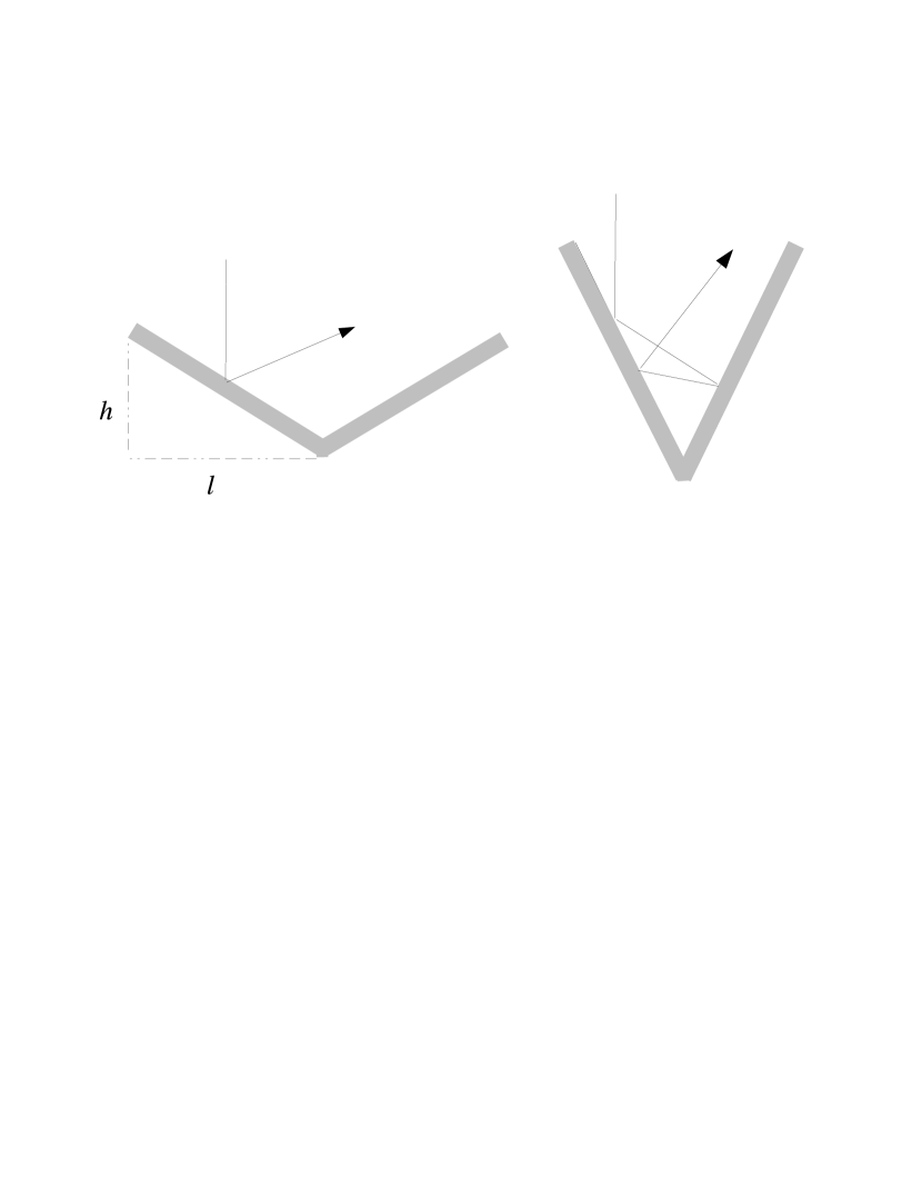
Figure 11.— Effect of surface roughness on the reflectivity. The surface roughness is characterized by the vertical scale $h$ and horizontal scale $l$, both much greater than the photon wavelength. For the idealized “triangular” surface, a normal incident ray goes through at least two reflections if $\theta=\tan^{-1}(l/h)<60^{\circ}$, at least three reflections if $\theta<36^{\circ}$, at least four reflections if $\theta<180^{\circ}/7$, etc. Thus net reflectivity of the rough surface is $\ll 1$ if $h>{\rm a~{}few}\times l$, and the emission spectrum will be close to blackbody.

The emission from a condensed NS surface is distinct from atmospheric emission in several aspects: (i) Atmospheric emission generally possesses a hard spectral tail (although this tail is somewhat suppressed by the QED effect for $B\gtrsim 10^{14}$ G; see §1), whereas the condensed surface emission does not; (ii) The spectrum of a cool NS atmosphere can have both cyclotron and atomic absorption features (again, they are reduced for $B\gtrsim 10^{14}$ G); the broad (cyclotron and plasma) features of condensed surface emission persist even in the magnetar field regime (if they are not smoothed out by variations of surface B fields or by the rough surface effect); (iii) The polarization signature of condensed matter emission is qualitatively different from that of atmospheric emission. All these aspects can serve as diagnostics for the physical condition of the emission region.

At the surface temperature of AXPs and SGRs, $T\simeq 5\times 10^{6}$ K, H is unlikely to be condensed, but Fe condensation is possible. The dim, isolated NSs have lower temperatures ($T\lesssim 10^{6}$ K), and if they possess magnetar-like fields, condensation is likely. In particular, the black-body X-ray spectra of RX J1856.5$-$3754 ($kT\simeq 64$eV) and RX J0420$-$5022 ($kT\simeq 45$eV; see Haberl et al. 2004b) could arise from condensed surface emission (e.g., non-smooth Fe surface at $B\gtrsim 10^{12}$ G), although to account for the optical data, nonuniform surface temperatures are still needed.

Appendix A A. Reflectivity Calculation

Here we fill in some of the details for the reflectivity calculation described in §3.2.

In the coordinate system xyz defined in §3.2, the explicit expression for eq. (12) is:

$$\left[\begin{array}[]{cc}\epsilon\cos^{2}\theta_{B}+\eta\sin^{2}\theta_{B}+n_{j}^{2}(\sin^{2}\theta^{(t)}_{j}\cos^{2}\varphi-1)&i\,g\cos\theta_{B}+n_{j}^{2}\sin^{2}\theta^{(t)}_{j}\sin\varphi\,\cos\varphi\\ -i\,g\cos\theta_{B}+n_{j}^{2}\sin^{2}\theta^{(t)}_{j}\sin\varphi\cos\varphi&\epsilon+n_{j}^{2}(\sin^{2}\theta^{(t)}_{j}\sin^{2}\varphi-1)\\ (\epsilon-\eta)\sin\theta_{B}\cos\theta_{B}+n_{j}^{2}\sin\theta^{(t)}_{j}\cos\theta^{(t)}_{j}\cos\varphi&i\,g\,\sin\theta_{B}+n_{j}^{2}\sin\theta^{(t)}_{j}\cos\theta^{(t)}_{j}\sin\varphi\\ \end{array}\right.$$ (A4)

$$\left.\begin{array}[]{c}(\epsilon-\eta)\sin\theta_{B}\cos\theta_{B}+n_{j}^{2}\sin\theta^{(t)}_{j}\cos\theta^{(t)}_{j}\cos\varphi\\ -i\,g\sin\theta_{B}+n_{j}^{2}\sin\theta^{(t)}_{j}\cos\theta^{(t)}_{j}\sin\varphi\\ \epsilon\sin^{2}\theta_{B}+\eta\cos^{2}\theta_{B}-n_{j}^{2}\sin^{2}\theta^{(t)}_{j}\end{array}\right]\cdot\left[\begin{array}[]{c}E_{x}\\ E_{y}\\ E_{z}\end{array}\right]\ =\ {\bf 0},$$ (A11)

where $n_{j}$ (with $j=1,2$) is the index of refraction in the medium, and $\theta_{j}^{(t)}$ is the formal complex angle of propagation calculated using Snell’s law (see Appendix B for a discussion of the interpretation of complex $\theta^{(t)}_{j}$). Taking the determinant of eq. (A4) yields:

$$a_{4}n_{j}^{4}+a_{2}n_{j}^{2}+\cos\theta^{(t)}_{j}\sin\theta^{(i)}\left(a_{1}n_{j}+a_{3}n^{3}_{j}\right)+a_{0}=0,$$ (A12)

where we have used Snell’s law and the following definitions:

$$a_{0} = (\epsilon^{2}-g^{2})\eta+{1\over 8}\left[g^{2}+\epsilon(\eta-\epsilon)\right]\left(2+6\cos 2\theta_{B}-4\sin^{2}\theta_{B}\cos 2\varphi\right)\sin^{2}\theta^{(i)}$$ (A13a)

$$-2\left(\epsilon\cos^{2}\theta_{B}+\eta\sin^{2}\theta_{B}\right)\sin^{2}\varphi\sin^{4}\theta^{(i)}$$

$$a_{1} = \left[\epsilon(\eta-\epsilon)+g^{2}\right]\sin 2\theta_{B}\cos\varphi$$ (A13b)

$$a_{2} = {1\over 2}\left[g^{2}-\epsilon(\epsilon+3\eta)-(g^{2}+\epsilon(\eta-\epsilon))\cos 2\theta_{B}\right]+$$ (A13c)

$$\left[\epsilon(\epsilon-\eta)\cos 2\theta_{B}+(\epsilon\cos^{2}\theta_{B}+\eta\sin^{2}\theta_{B})\sin^{2}\varphi-\epsilon\cos^{2}\varphi\right]\sin^{2}\theta^{(i)}$$

$$a_{3} = (\epsilon-\eta)\sin 2\theta_{B}\cos\varphi$$ (A13d)

$$a_{4} = \left(\epsilon^{2}-g^{2}\right)\eta.$$ (A13e)

The $\cos\theta^{(t)}_{j}$ term is moved to the right-hand side, and the entire equation is then squared. Using the identity $\cos^{2}\theta^{(t)}_{j}=1-\sin^{2}\theta^{(t)}_{j}$ and Snell’s law gives a polynomial equation in $n_{j}$:

$$a_{4}^{2}n_{j}^{8}+(2a_{2}a_{4}-a_{3}^{2}\sin^{2}\theta^{(i)})n_{j}^{6}+(a_{2}^{2}+2a_{0}a_{4}-2a_{1}a_{3}\sin^{2}\theta^{(i)}+a_{3}^{2}\sin^{4}\theta^{(i)})n_{j}^{4}+$$

$$(2a_{0}a_{2}-a_{1}^{2}\sin^{2}\theta^{(i)}+2a_{1}a_{3}\sin^{4}\theta^{(i)})n_{j}^{2}+a_{0}^{2}+a_{1}^{2}\sin^{4}\theta^{(i)}\ =\ 0$$ (A14)

The polynomial equation (A) has eight roots for $n_{j}$ which we found numerically using Laguerre’s method (Press et al, 1996). Only two of the roots are physical and satisfy the original equation (A12). In practice, it was found that for certain combinations of the parameters $E$, $\theta^{(i)}$, $\theta_{B}$, $\varphi$, a spurious root satisfies eqn. (A12) to the specified degree of accuracy, resulting in an unphysical result for the reflectivity. It is often the case that such roots can be discounted physically using the conditions (B3) and (B4) (see Appendix B). Once the indices of refraction $n_{1}$, $n_{2}$ are known, the normal mode polarization vectors can be determined. Solving eqn. (12) for the ratios $E^{(t)}_{x}/E^{(t)}_{y}$ and $E^{(t)}_{z}/E^{(t)}_{y}$ gives the expressions:

$$f_{j}=\left({E^{(t)}_{x}\over E^{(t)}_{y}}\right)_{j} = i\,{{\epsilon-i\,B_{j}\,g\sin\theta_{B}+n_{j}^{2}\sin\theta^{(t)}_{j}\sin\varphi\left(B_{j}\cos\theta^{(t)}_{j}+\sin\theta^{(t)}_{j}\sin\varphi\right)-n_{j}^{2}}\over{g\cos\theta_{B}+A_{j}\,g\sin\theta_{B}+i\,n_{j}^{2}\sin\theta^{(t)}_{j}\left(A_{j}\cos\theta^{(t)}_{j}+\sin\theta^{(t)}_{j}\cos\varphi\right)\sin\varphi}},$$ (A15a)

$$g_{j}=\left({E^{(t)}_{z}\over E^{(t)}_{y}}\right)_{j} = A_{j}\left(E^{(t)}_{x}\over E^{(t)}_{y}\right)_{j}+B_{j},$$ (A15b)

$$A_{j} = -{{\epsilon\cos^{2}\theta_{B}+\eta\sin^{2}\theta_{B}+n_{j}^{2}\sin^{2}\theta^{(t)}_{j}\cos^{2}\varphi}\over{(\epsilon-\eta)\sin\theta_{B}\cos\theta_{B}+n_{j}^{2}\sin\theta^{(t)}_{j}\cos\theta^{(t)}_{j}\cos\varphi}},$$ (A15c)

$$B_{j} = -{i\,g\cos\theta_{B}+n_{j}^{2}\sin\theta^{(t)}_{j}\sin\varphi\cos\varphi\over(\epsilon-\eta)\sin\theta_{B}\cos\theta_{B}+n_{j}^{2}\sin\theta^{(t)}_{j}\cos\theta^{(t)}_{j}\cos\varphi}.$$ (A15d)

With the propagation modes in the plasma determined, the latter two equations of (14) give:

$$\left(\begin{array}[]{cccc}\cos\theta^{(i)}\sin\varphi&\cos\varphi&C_{1}&C_{2}\\ \cos\theta^{(i)}\cos\varphi&\sin\varphi&-C_{1}&-C_{2}\\ -\cos\varphi&-\cos\theta^{(i)}\sin\varphi&C_{5}&C_{6}\\ -\sin\varphi&\cos\theta^{(i)}\cos\varphi&C_{7}&C_{8}\end{array}\right)\cdot\left\{\begin{array}[]{c}\left(\begin{array}[]{c}r_{11}\\ r_{12}\\ t_{11}\\ t_{12}\end{array}\right)\\ \left(\begin{array}[]{c}r_{21}\\ r_{22}\\ t_{21}\\ t_{22}\end{array}\right)\end{array}\right.=\left.\begin{array}[]{c}\left(\begin{array}[]{c}-\cos\theta^{(i)}\sin\varphi\\ \cos\theta^{(i)}\cos\varphi\\ \cos\varphi\\ \sin\varphi\end{array}\right)\\ \left(\begin{array}[]{c}-\cos\varphi\\ -\sin\varphi\\ -\cos\theta^{(i)}\sin\varphi\\ \cos\theta^{(i)}\cos\varphi\end{array}\right)\end{array}\right.$$ (A16)

for the incoming polarization modes ${\bf e}^{(i)}_{1}=(-\cos\theta^{(i)}\cos\varphi,-\cos\theta^{(i)}\sin\varphi,\sin\theta^{(i)})$ and ${\bf e}^{(i)}_{2}=(\sin\varphi,-\cos\varphi,0)$. Inverting the coefficient matrix of eqn. (A16) and performing extensive algebra yields the following expressions for the reflected field amplitudes:

$$r_{11} = {{4A\cos\theta^{(i)}-2B_{-}\sin^{2}\theta^{(i)}+(3+\cos 2\theta^{(i)})(B_{+}\cos 2\varphi+C_{+}\sin 2\varphi)}\over{4A\cos\theta^{(i)}+B_{-}(3+\cos 2\theta^{(i)})-2\sin^{2}\theta^{(i)}(B_{+}\cos 2\varphi+C_{+}\sin 2\varphi)}},$$ (A17a)

$$r_{12} = {{4\cos\theta^{(i)}(C_{-}+B_{+}\sin 2\varphi-C_{+}\cos 2\varphi)}\over{4A\cos\theta^{(i)}+B_{-}(3+\cos 2\theta^{(i)})-2\sin^{2}\theta^{(i)}(B_{+}\cos 2\varphi+C_{+}\sin 2\varphi)}},$$ (A17b)

$$r_{21} = {{4\cos\theta^{(i)}(C_{+}\cos 2\varphi-B_{+}\sin 2\varphi+C_{-})}\over{4A\cos\theta^{(i)}+B_{-}(3+\cos 2\theta^{(i)})-2\sin^{2}\theta^{(i)}(B_{+}\cos 2\varphi+C_{+}\sin 2\varphi)}},$$ (A17c)

$$r_{22} = {{(3+\cos 2\theta^{(i)})(B_{+}\cos 2\varphi+C_{+}\sin 2\varphi)-4A\cos\theta^{(i)}-2B_{-}\sin^{2}\theta^{(i)}}\over{4A\cos\theta^{(i)}+B_{-}(3+\cos 2\theta^{(i)})-2\sin^{2}\theta^{(i)}(B_{+}\cos 2\varphi+C_{+}\sin 2\varphi)}},$$ (A17d)

using the definitions:

$$C_{1,2} = \left[1+\left|f_{1,2}\right|^{2}+\left|g_{1,2}\right|^{2}\right]^{-1/2},$$ (A18a)

$$C_{5,6} = C_{1,2}\left[n_{1,2}\,\sin\theta^{(t)}_{1,2}\,\cos\varphi\,g_{1,2}-n_{1,2}\,\cos\theta^{(t)}_{1,2}\,f_{1,2}\right],$$ (A18b)

$$C_{7,8} = C_{1,2}\left[n_{1,2}\,\sin\theta_{1,2}^{(t)}\,\sin\varphi\,g_{1,2}-n_{1,2}\,\cos\theta_{1,2}^{(t)}\right],$$ (A18c)

$$A = (C_{6}C_{7}-C_{5}C_{8}),$$ (A18d)

$$B_{\pm} = (C_{2}C_{5}+C_{2}C_{6})\pm(C_{2}C_{7}-C_{1}C_{8}),$$ (A18e)

$$C_{\pm} = (C_{1}C_{6}+C_{2}C_{5})\pm(C_{2}C_{7}-C_{1}C_{8}),$$ (A18f)

The reflectivity and the emission spectrum and polarization are then determined by eqs. (7), (8), and (9).

Appendix B B. Complex Angle of Propagation

In this Appendix we outline some of the physical properties of the wave propagating in the plasma with complex index of refraction (cf. Born & Wolf 1970, §13.2).

For a medium with complex index of refraction $n=n_{R}+in_{I}$ (where $n_{R}$ and $n_{I}$ are real), the formal refraction angle $\theta^{(t)}$, as determined by Snell’s law, is complex. Let $\cos\theta^{(t)}=(1-\sin^{2}\theta^{(t)})^{1/2}=\cos\theta^{(t)}_{R}+i\cos\theta^{(t)}_{I}$. Defining the vector parallel to the plane of incidence $\hat{\mbox{\boldmath$s$}}=(-\cos\varphi,-\sin\varphi,0)$, the wavevector for the transmitted waves can be written:

$${\bf k}^{(t)} = {n\omega\over c}\left(\sin\theta^{(t)}\hat{\mbox{\boldmath$s$}}-\cos\theta^{(t)}{\bf\hat{z}}\right)$$ (B1)

$$= {\omega\over c}\left[\sin\theta^{(i)}\hat{\mbox{\boldmath$s$}}+(n_{I}\cos\theta^{(t)}_{I}-n_{R}\cos\theta^{(t)}_{R}){\bf\hat{z}}-i(n_{I}\cos\theta^{(t)}_{R}+n_{R}\cos\theta^{(t)}_{I}){\bf\hat{z}}\right]$$

The transmitted electric field has the form $E^{(t)}\propto e^{i{\bf k}^{(t)}\cdot{\bf r}-i\omega t}$. Substituting eqn. (B1) into this expression, the field takes the form:

$$E^{(t)} \propto \exp\left[(n_{R}\cos\theta^{(t)}_{I}+n_{I}\cos\theta^{(t)}_{R})z\right]\times$$ (B2)

$$\exp\left[i{\omega\over c}\left(\sin\theta^{(i)}s-(n_{R}\cos\theta^{(t)}_{R}-n_{I}\cos\theta^{(t)}_{I})z\right)-i\omega t\right].$$

Thus, the transmitted wave has a propagating component multiplied by a damping factor. Since the amplitude of the wave must decrease as it travels through the medium, eqn. (B2) gives the following condition on the index of refraction (recall that in the geometry of §3.2, $z<0$):

$$n_{R}\cos\theta^{(t)}_{I}+n_{I}\cos\theta^{(t)}_{R}>0.$$ (B3)

The traveling component can be used to define a new wavevector ${\bf k}^{\prime}=\sin\theta^{(i)}\hat{\mbox{\boldmath$s$}}-(n_{R}\cos\theta^{(t)}_{R}-n_{I}\cos\theta^{(t)}_{I}){\bf\hat{z}}$. The real angle of propagation is then given by $\cos\theta^{(t)^{\prime}}=\hat{{\bf k}^{\prime}}\cdot{\bf k}^{\prime}/|{\bf k}^{\prime}|$. By assumption, the angle of propagation for the refracted wave measured with respect to the $z$ axis must be greater than $\pi/2$, yielding a second condition on the index of refraction:

$$-1\leq\cos\theta^{(t)^{\prime}}={{n_{I}\cos\theta^{(t)}_{I}-n_{R}\cos\theta^{(t)}_{R}}\over{\sqrt{\sin^{2}\theta^{(i)}+(n_{I}\cos\theta^{(t)}_{I}-n_{r}\cos\theta^{(t)}_{R})^{2}}}}\leq 0.$$ (B4)

The real and imaginary parts of the indices of refraction for the birefringent transmitted waves must satisfy eqs. (B3) and (B4).

References

• Arras & Lai (1999) Arras, P., & Lai, D. 1999, Bull. of Amer. Astro. Soc., 31, 739
• Ashcroft & Mermin (1976) Ashcroft, N., & Mermin, D. 1976, Solid Sate Physics (New York: Holt, Rinehart, and Winston)
• Born & Wolf (1970) Born, M., & Wolf, E. 1970, Principles of Optics (4th ed.; Oxford: Pergamon Press)
• Braje & Romani (2002) Braje, T.M., & Romani, R.W. 2002, ApJ, 580, 1043
• Brinkmann (1980) Brinkmann, W. 1980, A&A, 82, 352
• Burwitz et al. (2001) Burwitz, V., Zavlin, V.E., Neuhäuser, R., Predehl, P., Trümper, & J., Brinkman, A.C. 2001, A&A, 379, L35
• Burwitz et al. (2003) Burwitz, V., Haberl, F., Neuhäuser, R., Predehl, P., Trümper, J., & Zavlin, V.E. 2003, A&A, 399, 1109
• Canuto & Ventura (1972) Canuto, V., & Ventura, J. 1972, Ap. Space Sci., 18, 104
• Chabrier (1993) Chabrier, G. 1993, ApJ, 414, 695
• De Luca et al. (2004) De Luca, A., Mereghetti, S., Caraveo, P.A., Moroni, M., Mignani, R.P., & Bignami, G.F. 2004, A&A, 418, 625
• Drake et al. (2002) Drake, J., et al. 2002, ApJ, 572, 996
• Flowers et al. (1977) Flowers, E.G., Lee, J.-F., Ruderman, M.A., Sutherland, P.G., Hillebrandt, W., & Müller, E. 1977, ApJ, 215, 291
• Ginzburg (1970) Ginzburg, V.L. 1970, Propagation of Electromagnetic Waves in Plasmas (2d ed.; Oxford: Pergamon Press)
• Haberl et al. (2003) Haberl, F., Schwope, A.D., Hambaryan, V., Hasinger, G., & Motch, C. 2003, A&A, 403, L19
• Haberl et al. (2004a) Haberl, F., Zavlin, V.E., Trümper, J., & Burwitz, V. 2004a, A&A, 419, 1077
• Haberl et al. (2004b) Haberl, F., Motch, C., Zavlin, V.E., Gänsicke, B.T., Cropper, M., Schwope, A.D., Turolla, R., & Zane, S. 2004b, A&A, 424, 635
• Hailey & Mori (2002) Hailey, C. J., & Mori, K. 2002, ApJ, 578, L133
• Ho & Lai (2003) Ho, W.C.G., & Lai, D. 2003, MNRAS, 338, 233
• Ho & Lai (2004) Ho, W.C.G., & Lai, D. 2004, ApJ, 607, 420
• Ho et al. (2003) Ho, W.C.G., Lai, D., Potekhin, A.Y., & Chabrier, G. 2003, ApJ, 599, 1293
• Hubbard (1966) Hubbard, W. B. 1966, ApJ 146, 858
• Itoh (1975) Itoh, N. 1975, MNRAS, 173, 1P
• Jones (1986) Jones, P.B. 1986, MNRAS, 218, 477
• Juett et al. (2002) Juett, A.M., Marshall, H.L., Chakrabarty, D., & Schulz, N.S. 2002, ApJ, 568, L31
• Kadomtsev (1970) Kadomtsev, B.B., 1970, Zh. Eksp. Teor. Fiz, 58, 1765 [Sov. Phys. JETP 31, 945 (1970)]
• Lai (2001) Lai, D. 2001, Review of Modern Physics, 73, 629
• Lai & Ho (2002) Lai, D., & Ho, W.C.G. 2002, ApJ, 566, 373
• Lai & Ho (2003a) Lai, D., & Ho, W.C.G. 2003a, ApJ, 588, 962
• Lai & Ho (2003b) Lai, D., & Ho, W.C.G. 2003b, Phys. Rev. Lett. 91, 071101
• Lai & Salpeter (1997) Lai, D., & Salpeter, E.E. 1997, ApJ, 491, 270
• Lenzen & Trümper (1978) Lenzen, R., & Trümper, J. 1978, Nature, 271, 216
• Lloyd (2003) Lloyd, D. 2003, MNRAS, submitted (astro-ph/0303561)
• Mereghetti et al. (2002) Mereghetti, S., De Luca, A., Caraveo, P.A., Becker, W., Mignani, R., & Bignami, G.F. 2002, ApJ, 581, 1280
• Mori & Hailey (2003) Mori, K., & Hailey, C. 2003, ApJ, submitted (astro-ph/0301161)
• Mori & Ruderman (2003) Mori, K., & Ruderman, M. 2003, ApJ, 592, L75
• Morii et al. (2003) Morii, M., Sato, R., Kataoka, J., & Kawai, N. 2003, PASJ, 55, L45
• Müller (1984) Müller, E. 1984, A&A, 130, 415
• Neuhauser et al. (1987) Neuhauser, D., Koonin, S.E., & Langanke, K. 1987, Phys. Rev. A, 36, 4163
• Ogata & Ichimaru (1990) Ogata, S., & Ichimaru, S. 1990, Phys. Rev. A, 42, 4867
• Paerels et al. (2001) Paerels, F., Rasmussen, A.P., Hartmann, H.W., Heise, J., Brinkman, A.C., de Vries, C.P., & den Herder, J.W. 2001, A&A, 365, L298
• Patel et al. (2003) Patel, S.K., et al. 2003, ApJ, 587, 367
• Pavlov & Zavlin (2003) Pavlov, G. G., & Zavlin, V. E. 2003, in XXI Texas Symposium on Relativistic Astrophysics, ed. R. Bandiera et al (Singapore: World Scientific), 319
• Pavlov et al. (1980) Pavlov, G. G., Shibanov, Yu. A, & Yakovlev, D. G. 1980, Ap. Space Sci., 73, 33
• Perez-Azorin et al. (2004) Perez-Azorin, J.F., Miralles, J.A., Pons, J.A. 2004, A&A, submitted (astro-ph/0410664)
• Pons et al. (2002) Pons, J.A., Walter, F.M., Lattimer, J.M., Prakash, M., Neuhäuser, R., & An, P. 2002, ApJ, 564, 981
• Potekhin (1999) Potekhin, A.Y. 1999, A&A, 351, 787
• Potekhin & Chabrier (2000) Potekhin, A.Y., & Chabrier, G. 2000, Phys. Rev. E, 62, 8554
• Potekhin & Chabrier (2003) Potekhin, A.Y., & Chabrier, G. 2003, ApJ, 585, 955
• Potekhin & Chabrier (2004) Potekhin, A.Y., & Chabrier, G. 2004, ApJ, 600. 317
• Potekhin et al. (1999a) Potekhin, A.Y., Chabrier, G., & Shibanov, Yu.A. 1999a, Phys. Rev. E, 60, 2193
• Potekhin et al. (1999b) Potekhin, A.Y., Baiko, D.A., Haensel, P., & Yakovlev, D.G. 1999b, A&A, 346, 345
• Potekhin et al. (2004) Potekhin, A.Y., Lai, D., Chabrier, G., & Ho, W.C.G. 2004, ApJ, 612, 1034
• Rajagopal & Romani (1996) Rajagopal, M., & Romani, R.W. 1996, ApJ, 461, 327
• Sanwal et al. (2002) Sanwal, D., Pavlov, G.G., Zavlin, V.E., & Teter, M.A. 2002, ApJ, 574, L61
• Ruderman (1971) Ruderman, M. 1971, Phys. Rev. Lett. 27, 1306
• Shibanov et al. (1992) Shibanov, Yu.A., Zavlin, V.E., Pavlov, G.G., & Ventura, J. 1992, A&A, 266, 313
• Tiengo et al. (2002) Tiengo, A., Göhler, E., Staubert, R., & Mereghetti, S. 2002, A&A, 383, 182
• Trümper et al. (2003) Trümper, J.E., et al. 2003, astro-ph/0312600
• Turolla et al. (2004) Turolla, R., Zane, S., & Drake, J.J. 2004, ApJ, 603, 265
• Usov et al. (1980) Usov, N.A., Grebenshchikov, Yu.B, & Ulinich, F.R. 1980, Sov. Phys.–JETP, 51, 148
• van Kerkwijk et al. (2004) van Kerkwijk, M.H., Kaplan, D.L., Durant, M., Kulkarni, S.R., & Paerels, F. 2004, ApJ, 608, 432
• Walter et al. (1996) Walter, F., Wolk, S.J., & Neuhauser, R. 1996, Nature, 379, 233
• Ziman (1979) Ziman, J.M. 1979, Principles of the Theory of Solids (Cambridge Univ. Press)