Number Counts At $3<\lambda<10\micron$ from the Spitzer Space Telescope

Abstract

Infrared source counts at wavelengths $3<\lambda<10$ µm cover more than 10 magnitudes in source brightness, four orders of magnitude in surface density, and reach an integrated surface density of $10^{5}$ sources deg^-2. At $m<14$ mag, most of the sources are Galactic stars, in agreement with models. After removal of Galactic stars, galaxy counts are consistent with what few measurements exist at nearby wavelengths. At 3.6 and 4.5 µm, the galaxy counts follow the expectations of a Euclidean world model down to $\sim$16 mag and drop below the Euclidean curve for fainter magnitudes. Counts at these wavelengths begin to show decreasing completeness around magnitude 19.5. At 5.8 and 8 µm, the counts relative to a Euclidean world model show a large excess at bright magnitudes. This is probably because local galaxies emit strongly in the aromatic dust (“PAH”) features. The counts at 3.6 µm resolve $<$50% of the Cosmic Infrared Background at that wavelength.

1 Introduction

Extragalactic galaxy counts are one of the four “classical” tests of observational cosmology because they sample the variation in the volume element with increasing luminosity distance to the source. Optical galaxy counts flourished in the last several decades (e.g., Tyson & Jarvis, 1979; Williams et al., 1996) with the advent of charge-coupled devices. Near-infrared counts arrived in the last decade (e.g., Djorgovski et al., 1995; Yan et al., 1998) with the availability of large format detectors. However, the original cosmological goals have been supplanted by the realization that galaxy evolution plays a major role in the results. The optical counts in particular demonstrated the faint blue galaxy problem—that there were too many faint blue galaxies compared to predictions based on the local luminosity function.

In order to understand the effects of galaxy evolution on counts, it is essential to have counts at a wide range of wavelengths because there are many types of galaxies that emit at different wavelengths over their lifetimes. For example, normal galaxies alone cannot explain the cosmic infrared background (Hauser & Dwek, 2001); instead, it is necessary to invoke a population of dusty, starbursting galaxies (e.g., M82) which re-radiate a substantial portion of their bolometric luminosity in the far-infrared. Such galaxies also exhibit mid-infrared colors redder than normal galaxies (e.g., Rigopoulou et al., 1999). Active galactic nuclei have redder colors than normal galaxies in the near infrared (e.g., 1.2 to 3.5 µm Ward et al., 1987). Populations of both starbursting galaxies and AGN have been predicted to be key components of the extragalactic number counts at wavelengths $>$3µm. Some models predict vastly different numbers of galaxies at 6.7 µm versus the $K$-band at 2.2µm. For example, compare the models of Franceschini et al. (1994), Xu et al. (2001), Rowan-Robinson (2001), Malkan & Stecker (2001), and Pearson & Rowan-Robinson (1996), which differ by $\sim$1 dex in integrated number counts at $F_{6.7}\sim 1$ mJy (although they differ less at fainter fluxes). Though all these models show reasonable agreement with the many observations of number counts at 2.2 µm, the disagreement at slightly longer wavelengths demonstrates that existing data are insufficient to constrain the models.

Mid-infrared measurements of galaxy counts are exceedingly difficult to make from the ground because of high thermal background emission and the limited wavelength regions that the atmosphere is transparent. Nonetheless, Hogg et al. (2000) detected nine extragalactic sources to a limit of 17.5 mag (33 $\mu$Jy) at 3.2µm. Observations at mid-infrared wavelengths are better made from space, where the thermal background is low and stable. The Infrared Space Observatory mission led to the first observations of galaxy counts at 6.75µm (Oliver et al., 1997), reaching 15.8 mag (40 $\mu$Jy) in the Hubble Deep Field. Similar observations (or up to 0.2 mag deeper) were reported by Taniguchi et al. (1997) for the Lockman Hole, Flores et al. (1999) for the CFRS 1415+52 field (part of the EGS, discussed below), and Oliver et al. (2002) for the Hubble Deep Field South. Altieri et al. (1999) observed a lensing cluster (A2390) to about the same depth on the sky but detected intrinsically fainter sources because of the lens amplification. Sato et al. (2003) reached sources as faint as 17.8 mag (6 $\mu$Jy) in the SSA 13 region. Serjeant et al. (2000) took a different approach, surveying to only 12.3 mag (1 mJy) but covering a large area of 6.5 deg².

Here, we report the first source counts at $3<\lambda<10$ µm made with the InfraRed Array Camera (IRAC) instrument on the Spitzer Space Telescope. With the low background available in space, the instrument can reach faint limiting fluxes in modest exposure times. In fact, IRAC can reach similar depths (19th magnitude) as the 10 m W. M. Keck Telescope with the NIRC2 camera at $\sim$ 3.6 µm in only one-hundredth of the exposure time and does so with a far larger field of view: $5^{\prime}\times 5^{\prime}$ versus $40^{\prime\prime}\times 40^{\prime\prime}$.

In order to cover a wide range of magnitudes and counts, we combine data from three survey fields of complementary area and depth. We first present the raw source counts, which give the first comprehensive picture of the infrared sky at these wavelengths and sensitivities. We then subtract the Galactic stellar contribution to derive the extragalactic source counts. Quantitative data in this paper are given in instrumental magnitudes relative to Vega, the units least dependent on calibration uncertainties. The flux density of Vega in the IRAC bandpasses is $(277.5,179.5,116.6,63.1)$ Jy (Fazio et al., 2004).

2 Observations and data analysis

The deepest image used here (Barmby et al., 2004) is of a $5^{\prime}\times 10^{\prime}$ field surrounding the QSO HS 1700+6416 (hereafter QSO1700). Heavily dithered coverage allowed removal of spurious sources such as cosmic rays, instrumental artifacts due to bright stars, and the wings of bright stars. The resulting average exposure time at each point in the field was 7.8 hours. Object detection used SExtractor (Bertin & Arnouts, 1996) with the detection threshold set to 2.5$\sigma$ and the minimum area 5 pixels (3.6, 4.5 $\mu$m) or 7 pixels (5.8, 8.0 $\mu$m). Objects without a central peak (bright star wings) or sets of objects that appeared in a line (‘muxbleed’ or ‘banding’ artifacts) were removed. The 5$\sigma$ depth reached was 22.0, 21.5, 20.4, 19.6 mag (0.4, 0.5, 0.8, and 0.9 $\mu$Jy) respectively at the four IRAC wavelengths 3.6, 4.5, 5.8, and 8.0 µm (Barmby et al., 2004). Custom IDL software was used to measure magnitudes of detected objects in $1\farcs 5$ and $3\farcs 0$ radius circular apertures with sky annuli of $25\arcsec<r<35\arcsec$. A correction to a $12\farcs 2$ radius aperture (the standard aperture for observations of IRAC calibration stars) was derived using curves of growth based on the in-flight IRAC point spread function.

The intermediate depth image covers $0\fdg 17\times 2\arcdeg$ in the Extended Groth Strip (hereafter EGS). Data processing and photometry were the same as for the QSO1700 field. Depth of coverage was 26 frames of 200-s each reaching 5$\sigma$ limits of 21.5, 21.0, 18.5, 17.9 mag (0.7, 0.7, 4.6, 4.4 $\mu$Jy) at the four IRAC wavelengths.

The widest area survey covers $\sim 3\arcdeg\times 3\arcdeg$ in the Boötes region of the “NOAO Deep-Wide Survey” (Jannuzi & Dey, 1999). Depth of coverage is three 30-s IRAC frames at each point. Because of the minimal dithering, all sky positions having fewer than three individual images in agreement were removed from the mosaic to avoid having chance coincidences of cosmic rays “detected” as objects. The limiting magnitudes for 5$\sigma$ detection are 18.4, 17.7, 15.5, and 14.8 (12, 15, 74, 76 $\mu$Jy) at the four IRAC wavelengths (Eisenhardt et al., 2004). Source magnitudes were measured with SExtractor. The bright end number counts, which mostly refer to stars, are limited by saturation at magnitudes of 10.0, 9.8, 7.5, 7.7 (28, 22, 117, 52 mJy).

Table 1 (columns 2, 6, and 11) and Figure 1 show the resulting number counts for each field.

In order to use the number counts to study galaxy evolution, stars must be subtracted. At bright magnitudes (Boötes field), the spatial extent of brighter galaxies is big enough to separate them from stars using the difference between aperture magnitudes and “magauto” (which is roughly an isophotal magnitude) generated by SExtractor. Near the bright limit of the survey, the distant wings of the stellar PSF are bright enough to be seen, and bright stars are classed as galaxies by the automated software. Therefore the few sources in this brightness range were examined and classified visually. At fainter magnitudes, $m\gtrsim 14.5$ mag, morphology can no longer easily separate stars and galaxies at our image resolution of $\geq$1$\farcs$7 FWHM. The stellar contribution to the total source counts at these magnitudes, however, is small, so their number can be estimated statistically. Table 1 shows measured star counts (column 4) for the Boötes field and model star counts (columns 8 and 13) for the two deeper fields. The model (Arendt et al., 1998) is similar to one by Wainscoat et al. (1992) but with additional geometric details and extended source colors. The model matches the unresolved Galactic emission seen by DIRBE but may not accurately predict actual star counts in all lines of sight. Despite that, for $m>16.5$ mag, stars are a negligible fraction of the total counts. In the troublesome region $14.5<m<16.5$ mag, results for different fields and methods agree, and the galaxy counts do not change slope, but the extragalactic counts may be less accurate than in other ranges.

At the faintest levels, all surveys fail to detect some objects brighter than the ostensible limiting magnitude. This incompleteness is estimated by inserting artificial sources into the sky images and finding their recovery rate as a function of magnitude. For the EGS and QSO1700 fields, we used the usual ‘Monte Carlo’ method: scaling images of objects in the field to fainter fluxes, inserting them in the images in sets of 200, re-running SExtractor, and counting the number of artificial objects recovered. Objects were considered to be recovered if they were detected within 1.5 pixels and 0.5 mag of their input positions and magnitudes. Source counts were truncated at the faint end when the incompleteness exceeded 50%. The results are shown in Table 1 (columns 9 and 14).

The incompleteness in the 3.6 and 4.5 µm images does not show the usual rapid increase near the magnitude limit of the images but rather shows a gradual increase that begins at bright magnitudes $([3.6],[4.5])\approx(17.5,17.0)$. Furthermore, the incompleteness curves at these two wavelengths are very similar for both the EGS and QSO1700 fields, despite the differing exposure times by a factor of $>$5. Both of these features of the data are consistent with the images being affected by source confusion at their faint limits. For this reason, we choose to truncate the source counts at a relatively bright magnitude $[3.6]=[4.5]=20.5$ mag. This corresponds to integral counts of $\sim$36 beams/source. We caution against any over-interpretation of our results at the faintest magnitudes due to the complications arising from the source confusion. An improved analysis—using more sophisticated image combination algorithms, source detection, and more extensive Monte Carlo incompleteness simulations—will be deferred to a future contribution.

The incompleteness factors at 5.8 and 8 µm show sharper declines near the faint limits at these wavelengths and significant improvement in the QSO1700 field compared to the EGS field. Evidently the images at these wavelengths are still not deep enough for confusion to be a strong factor. This is consistent with the integral source density of $\sim$60 beams/source to magnitude 18.

Incompleteness corrections were not calculated for the Boötes field because its faint flux limit overlaps the other surveys. The limit indicated in Table 1 is where the Boötes field counts drop below 95% of the counts expected from the EGS field.

Figure 1 shows that Galactic stars dominate the counts at the bright end but become much less important at $m>14.5$ mag. Approximately $(4.8\times 10^{4},7.3\times 10^{3},2.8\times 10^{2})$ sources were catalogued at $[3.6]<(17.25,20.75,20.75)$ mag in the Boötes, EGS, and QSO1700 fields, respectively. The incompleteness-corrected integrated source counts reach surface densities of $\sim(1.4\times 10^{5},1.2\times 10^{5},7.1\times 10^{4},6.8\times 10^{4})$ deg^-2 at the wavelengths of $(3.6,4.5,5.8,8.0)$ respectively. The QSO1700 field contains two galaxy clusters at redshifts of 0.25 and 0.44. These may contribute to increased counts in the $15.5<m<17$ range for this field.

3 Galaxy Counts

Figure 2 shows our best estimate of the extragalactic number counts with stars subtracted and completeness corrections included. Some of the previous galaxy counts at nearby wavelengths are also shown as are some simple models. There is general agreement with previous observations, although wavelength differences may affect the results. For example, the ISO LW2 filter overlaps considerably with both the 5.8 and 8.0 µm bandpasses of IRAC, but it shows consistency only with our 5.8 µm counts. This is most likely a result of the differing long wavelength cutoffs of the filters (8.5 µm for LW2 versus 9.5 µm for the IRAC $8\mu$m filter).

The 3.6 and 4.5 µm observations are best compared with ground-based $K$-band (2.2 µm) counts. There are many surveys in the literature, but the curve from Kochanek et al. (2001) represents all the data. The IRAC counts in the two bands are consistent with the prior observations with only a mean offset of $(K-[3.6])\sim 0.7$ mag being required to bring them into rough agreement at $[3.6]<17$ mag. Models that predict the 3.6 µm counts to differ markedly from the $K$-band counts can therefore be rejected. The various models plotted in Figure 2 demonstrate that there is no single model to date that can match the galaxy counts throughout the observed flux ranges and in all bandpasses simultaneously.

4 Discussion

The galaxy counts at 3.6 and 4.5 µm appear flat at $m\leq 16$ mag, consistent with a Euclidean world model. The $5.8$ and 8.0 µm counts, however, show a steep drop from $8<m<16$ mag. We attribute the drop to substantial contribution to the fluxes from the strong aromatic feature emission at 6.2 and 7.7 µm (e.g., Lu et al., 2003). The brightest galaxies tend to be local ones, and the emission features are within the IRAC bands. Fainter galaxies, on the other hand, tend to be at higher redshift, and at $z\geq 0.23$ the 7.7 µm feature is leaving the 8.0 µm IRAC band. In effect, these bands have a strong positive “K-correction” (decreasing intrinsic flux density) as redshift increases, as suggested by Aussel, Elbaz, & Cesarsky (1999) for the ISO 6.75 µm filter. The slopes have different shapes in the two bands, presumably because of the larger bandwidth of the 8 µm filter and the greater strength of the 7.7 µm feature relative to the 6.2 µm feature.

With these number counts, we can estimate the contribution of IRAC-detected galaxies to the cosmic infrared background (CIRB). The integrated galaxy counts (weighted according to uncertainties) in Table 1 correspond to 5.4, 3.5, 3.6, and 2.6 nW m^-2 sr^-1 at the four IRAC wavelengths. The 3.6 µm surface brightness is $<$50% of the estimated 12 nW m^-2 sr^-1 CIRB at this wavelength (Wright & Reese, 2000). At longer wavelengths (4.5 – 8 µm), no reliable direct measurements of the EBL exist because of the difficulty in accurately accounting for the zodiacal and Galactic foreground emission, which brighten rapidly at $\lambda\gtrsim 3.5$ µm. It may prove difficult to construct a model consistent with these resolved galaxy counts while producing enough far infrared flux to match the cosmic far-infrared background.

5 Summary

Source counts at $3<\lambda<10\mu$m taken with the IRAC instrument on the Spitzer Space Telescope demonstrate:

1. Galaxy counts follow the Euclidean expectation at brighter fluxes at $3.6$ and $4.5\mu$m;

2. Confusion begins to set in around 19.5 mag for the 3.6 and 4.5 µm images and present source extraction technique, but there is no evidence of confusion down to 18.5 mag at 5.8 µm and 18.0 mag at 8 µm;

3. Bright galaxy counts at 5.8 and 8.0 µm are more numerous than the Euclidean expectation, most likely due to PAH emission lines from low-redshift, star-forming galaxies;

4. No existing model matches the galaxy counts throughout the observed flux range and simultaneously in all the IRAC bandpasses.

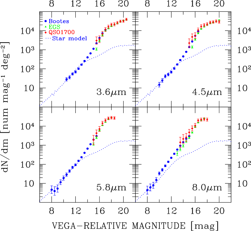
Figure 1: Differential number counts in the four IRAC bandpasses including all sources, stars and galaxies. Counts in the three fields are indicated by different colors. Only bins containing at least 10 sources are included. The dashed line shows stellar number counts predicted by the Faint Source Model as used by the DIRBE mission data analysis (Arendt et al., 1998) for the Boötes field. Stars dominate at the bright end of the counts but are a minor contributor at the faint end.

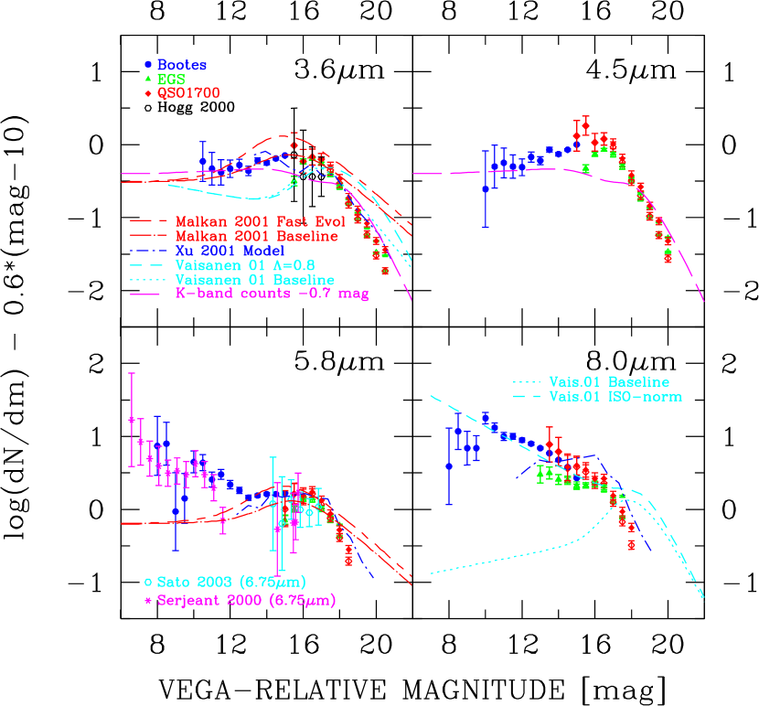
Figure 2: Extragalactic differential number counts in the four IRAC bandpasses normalized by the expected growth rate in a Euclidean Universe, i.e., $N(m)\times 10^{[-0.6(m-10)]}$. Open symbols are raw galaxy counts; filled symbols have the derived incompleteness correction applied. Stars were removed from the Boötes data using a morphological criterion and from the EGS and QSO1700 data statistically using the Galactic Faint Source Model (Arendt et al. 1998; see text). The 3.6 µm panel shows comparison data from Hogg et al. (2000, $3.2\mu$m) and the $K$-band number counts model from Kochanek et al. (2001), which is a good representation of the $K$-band data in this brightness range. The Kochanek et al. curve has been shifted by an arbitrary -0.7 mag to better match the 3.6 µm counts; this value could be interpreted as the average $K-[3.6]$ color for the galaxies contributing to the counts. The 5.8 µm panel contains comparison 6.75 µm counts from Serjeant et al. (2000) and Sato et al. (2003). Also plotted are models from Malkan & Stecker (2001, 3.6 and 5.8 µm), Xu et al. (2001, 3.6, 5.8, and 8 µm), and Väisänen, Tollestrup & Fazio (2001, 3.6 and 8 µm).

Table 1: IRAC Differential Number Counts

	Boötes				EGS					QSO1700
Magnitude	Total	$\pm$	Stars	Galaxies	Total	$\pm$	Stars	Comp.	Galaxies	Total	$\pm$	Stars	Comp.	Galaxies
1	2	3	4	5	6	7	8	9	10	11	12	13	14	15
$\lambda=3.6\mu$m
10.5	1.45	0.09	1.43	0.07	$\cdots$	$\cdots$	$\cdots$	$\cdots$	$\cdots$	$\cdots$	$\cdots$	$\cdots$	$\cdots$	$\cdots$
11.0	1.55	0.08	1.52	0.27	$\cdots$	$\cdots$	$\cdots$	$\cdots$	$\cdots$	$\cdots$	$\cdots$	$\cdots$	$\cdots$	$\cdots$
11.5	1.73	0.06	1.71	0.52	$\cdots$	$\cdots$	$\cdots$	$\cdots$	$\cdots$	$\cdots$	$\cdots$	$\cdots$	$\cdots$	$\cdots$
12.0	1.84	0.06	1.80	0.87	$\cdots$	$\cdots$	$\cdots$	$\cdots$	$\cdots$	$\cdots$	$\cdots$	$\cdots$	$\cdots$	$\cdots$
12.5	2.01	0.05	1.93	1.22	$\cdots$	$\cdots$	$\cdots$	$\cdots$	$\cdots$	$\cdots$	$\cdots$	$\cdots$	$\cdots$	$\cdots$
13.0	2.22	0.04	2.14	1.44	$\cdots$	$\cdots$	$\cdots$	$\cdots$	$\cdots$	$\cdots$	$\cdots$	$\cdots$	$\cdots$	$\cdots$
13.5	2.41	0.03	2.27	1.88	$\cdots$	$\cdots$	$\cdots$	$\cdots$	$\cdots$	$\cdots$	$\cdots$	$\cdots$	$\cdots$	$\cdots$
14.0	2.60	0.02	2.41	2.15	$\cdots$	$\cdots$	$\cdots$	$\cdots$	$\cdots$	$\cdots$	$\cdots$	$\cdots$	$\cdots$	$\cdots$
14.5	2.81	0.02	2.51	2.51	$\cdots$	$\cdots$	$\cdots$	$\cdots$	$\cdots$	$\cdots$	$\cdots$	$\cdots$	$\cdots$	$\cdots$
15.0	3.05	0.01	2.61	2.85	$\cdots$	$\cdots$	$\cdots$	$\cdots$	$\cdots$	$\cdots$	$\cdots$	$\cdots$	$\cdots$	$\cdots$
15.5	3.34	0.01	$\cdots$	$\cdots$	3.03	0.07	2.66	1.00	2.80	3.48	0.19	3.03	1.00	3.29
16.0	3.62	0.01	$\cdots$	$\cdots$	3.46	0.04	2.71	1.00	3.37	3.55	0.18	3.09	1.00	3.37
16.5	3.86	0.01	$\cdots$	$\cdots$	3.76	0.03	2.78	1.00	3.71	3.83	0.13	3.14	1.00	3.73
17.0	4.05	0.00	$\cdots$	$\cdots$	3.98	0.02	2.85	1.00	3.94	4.06	0.10	3.20	1.00	4.00
17.5	$\cdots$	$\cdots$	$\cdots$	$\cdots$	4.11	0.02	2.91	0.94	4.11	4.20	0.09	3.23	0.91	4.19
18.0	$\cdots$	$\cdots$	$\cdots$	$\cdots$	4.23	0.02	2.96	0.89	4.26	4.31	0.08	3.26	0.86	4.33
18.5	$\cdots$	$\cdots$	$\cdots$	$\cdots$	4.32	0.02	3.00	0.86	4.36	4.33	0.08	3.28	0.83	4.37
19.0	$\cdots$	$\cdots$	$\cdots$	$\cdots$	4.39	0.01	3.02	0.79	4.48	4.41	0.07	3.27	0.76	4.50
19.5	$\cdots$	$\cdots$	$\cdots$	$\cdots$	4.47	0.01	3.01	0.77	4.56	4.49	0.06	3.24	0.69	4.62
20.0	$\cdots$	$\cdots$	$\cdots$	$\cdots$	4.53	0.01	3.01	0.69	4.68	4.50	0.06	3.20	0.63	4.68
20.5	$\cdots$	$\cdots$	$\cdots$	$\cdots$	4.58	0.01	3.02	0.61	4.78	4.59	0.06	3.17	0.52	4.86
$\lambda=4.5\mu$m
10.0	1.17	0.12	1.16	-0.61	$\cdots$	$\cdots$	$\cdots$	$\cdots$	$\cdots$	$\cdots$	$\cdots$	$\cdots$	$\cdots$	$\cdots$
10.5	1.39	0.10	1.38	-0.00	$\cdots$	$\cdots$	$\cdots$	$\cdots$	$\cdots$	$\cdots$	$\cdots$	$\cdots$	$\cdots$	$\cdots$
11.0	1.61	0.08	1.58	0.35	$\cdots$	$\cdots$	$\cdots$	$\cdots$	$\cdots$	$\cdots$	$\cdots$	$\cdots$	$\cdots$	$\cdots$
11.5	1.70	0.07	1.66	0.60	$\cdots$	$\cdots$	$\cdots$	$\cdots$	$\cdots$	$\cdots$	$\cdots$	$\cdots$	$\cdots$	$\cdots$
12.0	1.83	0.06	1.78	0.89	$\cdots$	$\cdots$	$\cdots$	$\cdots$	$\cdots$	$\cdots$	$\cdots$	$\cdots$	$\cdots$	$\cdots$
12.5	2.02	0.05	1.92	1.33	$\cdots$	$\cdots$	$\cdots$	$\cdots$	$\cdots$	$\cdots$	$\cdots$	$\cdots$	$\cdots$	$\cdots$
13.0	2.23	0.04	2.12	1.58	$\cdots$	$\cdots$	$\cdots$	$\cdots$	$\cdots$	$\cdots$	$\cdots$	$\cdots$	$\cdots$	$\cdots$
13.5	2.46	0.03	2.27	2.03	$\cdots$	$\cdots$	$\cdots$	$\cdots$	$\cdots$	$\cdots$	$\cdots$	$\cdots$	$\cdots$	$\cdots$
14.0	2.65	0.02	2.42	2.27	$\cdots$	$\cdots$	$\cdots$	$\cdots$	$\cdots$	$\cdots$	$\cdots$	$\cdots$	$\cdots$	$\cdots$
14.5	2.89	0.02	2.53	2.63	$\cdots$	$\cdots$	$\cdots$	$\cdots$	$\cdots$	$\cdots$	$\cdots$	$\cdots$	$\cdots$	$\cdots$
15.0	3.14	0.01	2.58	3.00	$\cdots$	$\cdots$	$\cdots$	$\cdots$	$\cdots$	3.35	0.22	2.96	1.00	3.12
15.5	3.43	0.01	$\cdots$	$\cdots$	3.14	0.06	2.66	1.00	2.97	3.67	0.16	3.03	1.00	3.56
16.0	3.73	0.01	$\cdots$	$\cdots$	3.54	0.04	2.71	1.00	3.47	3.74	0.15	3.09	1.00	3.63
16.5	3.96	0.01	$\cdots$	$\cdots$	3.86	0.03	2.78	1.00	3.83	4.03	0.11	3.14	1.00	3.98
17.0	$\cdots$	$\cdots$	$\cdots$	$\cdots$	4.08	0.02	2.85	0.93	4.08	4.22	0.09	3.20	0.92	4.21
17.5	$\cdots$	$\cdots$	$\cdots$	$\cdots$	4.20	0.02	2.91	0.91	4.22	4.29	0.08	3.23	0.89	4.31
18.0	$\cdots$	$\cdots$	$\cdots$	$\cdots$	4.31	0.02	2.96	0.89	4.35	4.34	0.08	3.26	0.84	4.38
18.5	$\cdots$	$\cdots$	$\cdots$	$\cdots$	4.37	0.01	3.00	0.83	4.43	4.43	0.07	3.28	0.77	4.52
19.0	$\cdots$	$\cdots$	$\cdots$	$\cdots$	4.43	0.01	3.02	0.77	4.53	4.45	0.07	3.27	0.72	4.56
19.5	$\cdots$	$\cdots$	$\cdots$	$\cdots$	4.49	0.01	3.01	0.67	4.64	4.49	0.07	3.24	0.65	4.65
20.0	$\cdots$	$\cdots$	$\cdots$	$\cdots$	4.55	0.01	3.01	0.64	4.73	4.46	0.07	3.20	0.57	4.68
$\lambda=5.8\mu$m
8.0	0.67	0.20	0.63	-0.33	$\cdots$	$\cdots$	$\cdots$	$\cdots$	$\cdots$	$\cdots$	$\cdots$	$\cdots$	$\cdots$	$\cdots$
8.5	0.60	0.22	0.60	0.00	$\cdots$	$\cdots$	$\cdots$	$\cdots$	$\cdots$	$\cdots$	$\cdots$	$\cdots$	$\cdots$	$\cdots$
9.0	0.73	0.19	0.71	-0.63	$\cdots$	$\cdots$	$\cdots$	$\cdots$	$\cdots$	$\cdots$	$\cdots$	$\cdots$	$\cdots$	$\cdots$
9.5	1.06	0.13	1.03	-0.15	$\cdots$	$\cdots$	$\cdots$	$\cdots$	$\cdots$	$\cdots$	$\cdots$	$\cdots$	$\cdots$	$\cdots$
10.0	1.28	0.11	1.16	0.65	$\cdots$	$\cdots$	$\cdots$	$\cdots$	$\cdots$	$\cdots$	$\cdots$	$\cdots$	$\cdots$	$\cdots$
10.5	1.46	0.09	1.31	0.94	$\cdots$	$\cdots$	$\cdots$	$\cdots$	$\cdots$	$\cdots$	$\cdots$	$\cdots$	$\cdots$	$\cdots$
11.0	1.65	0.07	1.54	1.01	$\cdots$	$\cdots$	$\cdots$	$\cdots$	$\cdots$	$\cdots$	$\cdots$	$\cdots$	$\cdots$	$\cdots$
11.5	1.84	0.06	1.66	1.38	$\cdots$	$\cdots$	$\cdots$	$\cdots$	$\cdots$	$\cdots$	$\cdots$	$\cdots$	$\cdots$	$\cdots$
12.0	1.97	0.05	1.78	1.54	$\cdots$	$\cdots$	$\cdots$	$\cdots$	$\cdots$	$\cdots$	$\cdots$	$\cdots$	$\cdots$	$\cdots$
12.5	2.18	0.04	1.97	1.76	$\cdots$	$\cdots$	$\cdots$	$\cdots$	$\cdots$	$\cdots$	$\cdots$	$\cdots$	$\cdots$	$\cdots$
13.0	2.37	0.03	2.15	1.96	$\cdots$	$\cdots$	$\cdots$	$\cdots$	$\cdots$	$\cdots$	$\cdots$	$\cdots$	$\cdots$	$\cdots$
13.5	2.60	0.02	2.31	2.29	$\cdots$	$\cdots$	$\cdots$	$\cdots$	$\cdots$	$\cdots$	$\cdots$	$\cdots$	$\cdots$	$\cdots$
14.0	2.82	0.02	2.41	2.61	$\cdots$	$\cdots$	$\cdots$	$\cdots$	$\cdots$	$\cdots$	$\cdots$	$\cdots$	$\cdots$	$\cdots$
14.5	3.05	0.01	2.50	2.91	$\cdots$	$\cdots$	$\cdots$	$\cdots$	$\cdots$	$\cdots$	$\cdots$	$\cdots$	$\cdots$	$\cdots$
15.0	3.29	0.01	2.48	3.22	3.05	0.07	2.60	0.98	2.86	3.28	0.24	2.96	0.96	3.02
15.5	3.48	0.01	$\cdots$	$\cdots$	3.39	0.05	2.66	0.96	3.31	3.63	0.17	3.03	0.96	3.52
16.0	$\cdots$	$\cdots$	$\cdots$	$\cdots$	3.77	0.03	2.71	0.95	3.75	3.85	0.13	3.09	0.94	3.79
16.5	$\cdots$	$\cdots$	$\cdots$	$\cdots$	4.04	0.02	2.78	0.92	4.05	4.15	0.10	3.14	0.92	4.14
17.0	$\cdots$	$\cdots$	$\cdots$	$\cdots$	4.21	0.02	2.85	0.92	4.23	4.30	0.08	3.20	0.89	4.32
17.5	$\cdots$	$\cdots$	$\cdots$	$\cdots$	4.35	0.01	2.91	0.82	4.42	4.41	0.07	3.23	0.87	4.44
18.0	$\cdots$	$\cdots$	$\cdots$	$\cdots$	4.44	0.01	2.96	0.69	4.59	4.44	0.07	3.26	0.78	4.52
18.5	$\cdots$	$\cdots$	$\cdots$	$\cdots$	$\cdots$	$\cdots$	$\cdots$	$\cdots$	$\cdots$	4.42	0.07	3.28	0.69	4.55
$\lambda=8.0\mu$m
8.0	0.65	0.21	0.62	-0.61	$\cdots$	$\cdots$	$\cdots$	$\cdots$	$\cdots$	$\cdots$	$\cdots$	$\cdots$	$\cdots$	$\cdots$
8.5	0.79	0.18	0.67	0.17	$\cdots$	$\cdots$	$\cdots$	$\cdots$	$\cdots$	$\cdots$	$\cdots$	$\cdots$	$\cdots$	$\cdots$
9.0	0.90	0.16	0.79	0.24	$\cdots$	$\cdots$	$\cdots$	$\cdots$	$\cdots$	$\cdots$	$\cdots$	$\cdots$	$\cdots$	$\cdots$
9.5	1.18	0.12	1.07	0.54	$\cdots$	$\cdots$	$\cdots$	$\cdots$	$\cdots$	$\cdots$	$\cdots$	$\cdots$	$\cdots$	$\cdots$
10.0	1.52	0.08	1.19	1.25	$\cdots$	$\cdots$	$\cdots$	$\cdots$	$\cdots$	$\cdots$	$\cdots$	$\cdots$	$\cdots$	$\cdots$
10.5	1.71	0.07	1.39	1.42	$\cdots$	$\cdots$	$\cdots$	$\cdots$	$\cdots$	$\cdots$	$\cdots$	$\cdots$	$\cdots$	$\cdots$
11.0	1.92	0.05	1.63	1.60	$\cdots$	$\cdots$	$\cdots$	$\cdots$	$\cdots$	$\cdots$	$\cdots$	$\cdots$	$\cdots$	$\cdots$
11.5	2.13	0.04	1.76	1.90	$\cdots$	$\cdots$	$\cdots$	$\cdots$	$\cdots$	$\cdots$	$\cdots$	$\cdots$	$\cdots$	$\cdots$
12.0	2.34	0.03	1.89	2.15	$\cdots$	$\cdots$	$\cdots$	$\cdots$	$\cdots$	$\cdots$	$\cdots$	$\cdots$	$\cdots$	$\cdots$
12.5	2.55	0.03	2.02	2.40	$\cdots$	$\cdots$	$\cdots$	$\cdots$	$\cdots$	$\cdots$	$\cdots$	$\cdots$	$\cdots$	$\cdots$
13.0	2.77	0.02	2.17	2.64	2.56	0.11	2.25	1.00	2.28	$\cdots$	$\cdots$	$\cdots$	$\cdots$	$\cdots$
13.5	2.97	0.02	2.28	2.87	2.80	0.09	2.37	1.00	2.60	3.15	0.27	2.66	1.00	2.99
14.0	3.16	0.01	2.39	3.08	2.97	0.07	2.45	1.00	2.81	3.33	0.23	2.77	1.00	3.19
14.5	3.34	0.01	2.47	3.28	3.20	0.06	2.53	0.96	3.11	3.41	0.21	2.87	0.95	3.28
15.0	3.47	0.01	2.43	3.43	3.39	0.04	2.60	0.94	3.34	3.67	0.16	2.96	0.95	3.60
15.5	$\cdots$	$\cdots$	$\cdots$	$\cdots$	3.66	0.03	2.66	0.94	3.64	3.88	0.13	3.03	0.93	3.84
16.0	$\cdots$	$\cdots$	$\cdots$	$\cdots$	3.96	0.02	2.71	0.92	3.97	4.03	0.11	3.09	0.91	4.02
16.5	$\cdots$	$\cdots$	$\cdots$	$\cdots$	4.18	0.02	2.78	0.89	4.22	4.29	0.08	3.14	0.88	4.32
17.0	$\cdots$	$\cdots$	$\cdots$	$\cdots$	4.31	0.02	2.85	0.85	4.37	4.34	0.08	3.20	0.81	4.39
17.5	$\cdots$	$\cdots$	$\cdots$	$\cdots$	4.40	0.01	2.91	0.51	4.68	4.36	0.08	3.23	0.72	4.47
18.0	$\cdots$	$\cdots$	$\cdots$	$\cdots$	$\cdots$	$\cdots$	$\cdots$	$\cdots$	$\cdots$	4.34	0.08	3.26	0.56	4.55

Note. — Columns labelled “Total” tabulate the logarithm of the observed differential number counts in units of number mag^-1 deg^-2. Columns labeled “$\pm$” give the Poisson uncertainty of the total counts in logarithmic units. “Star” counts are in the same units. For the EGS and QSO1700 fields, the completeness (“Comp.”) estimated from the Monte Carlo simulations is tabulated and applied to the corresponding “Galaxy” counts. Total source counts are provided in the Boötes field fainter than stars and galaxies could be reliably separated using the morphology criterion (see text).

References

- Altieri et al. (1999) Altieri, B., et al. 1999, A&A, 343, L65
- Arendt et al. (1998) Arendt, R.G., et al. 1998, ApJ, 508, 74
- Aussel, Elbaz, & Cesarsky (1999) Aussel, H., Elbaz, D., & Cesarsky, C. J. 1999, Ap&SS, 266, 307
- Barmby et al. (2004) Barmby, P. et al. 2004, ApJS, this volume
- Bertin & Arnouts (1996) Bertin, E. & Arnouts, S. 1996, A&AS, 117, 393
- Davis et al. (2003) Davis, M., et al. 2003, Proc. SPIE, 4834, 161
- Djorgovski et al. (1995) Djorgovski, S. 1995, ApJ, 438, L13
- Eisenhardt et al. (2004) Eisenhardt, P. R. M., et al. 2004, ApJS, this volume
- Fazio et al. (2004) Fazio, G. G., et al. 2004, ApJS, this volume
- Flores et al. (1999) Flores, H., et al. 1999, ApJ, 517, 148
- Franceschini et al. (1994) Franceschini, A., Mazzei, P., de Zotti, G., & Danese, L. 1994, MNRAS, 427, 140
- Gardner, Cowie, & Wainscoat (1993) Gardner, J. P., Cowie, L. L., & Wainscoat, R. J. 1993, ApJ, 415, L9
- Hauser & Dwek (2001) Hauser, M.G., & Dwek, E. 2001, ARA&A, 39, 249
- Hogg et al. (2000) Hogg, D.W., Neugebauer, G., Cohen, J.G., Dickinson, M., Djorgovski, S., Matthews, K., & Soifer, B.T. 2000, AJ, 119, 1519
- Jannuzi & Dey (1999) Jannuzi, B.T. & Dey, A. 1999, in ASP Conf. Ser. 191, Photometric Redshifts and High Redshift Galaxies, ed. R. J. Weymann, L. J. Storrie-Lombardi, M. Sawicki, & R. J. Brunner (San Francisco: ASP), 111
- Kochanek et al. (2001) Kochanek, C.S., Pahre, M.A., Falco, E.E., Huchra, J.P., Mader, J., Jarrett, T.H., Chester, T., Cutri, R., & Schneider, S.E. 2001, ApJ, 560, 566
- Lu et al. (2003) Lu, N., Helou, G., Werner, M.W., Dinerstein, H.L., Dale, D.A., Silbermann, N.A., Malhotra, S., Beichman, C.A., & Jarrett, T.H. 2003, ApJ, 588, 199
- Malkan & Stecker (2001) Malkan, M. A. & Stecker, F. W. 2001, ApJ, 555, 641
- Oliver et al. (1997) Oliver, S. J., et al. 1997, MNRAS, 289, 471
- Oliver et al. (2002) Oliver, S., et al. 2002, MNRAS, 332, 536
- Pearson & Rowan-Robinson (1996) Pearson, C. Rowan-Robinson, M. 1996, MNRAS, 283, 174
- Peebles (2001) Peebles, P. J. E. 2001, International Journal of Modern Physics A, 16, 4223
- Rigopoulou et al. (1999) Rigopoulou, D., Spoon, H. W. W., Genzel, R., Lutz, D., Moorwood, A. F. M., & Tran, Q. D. 1999, AJ, 118, 2625
- Rowan-Robinson (2001) Rowan-Robinson, M. 2001, New Astronomy Reviews, 45, 631
- Sato et al. (2003) Sato, Y., et al. 2003, A&A, 405, 833
- Serjeant et al. (2000) Serjeant, S. et al. 2000, MNRAS, 316, 768
- Taniguchi et al. (1997) Taniguchi, Y., et al. 1997, A&A, 328, L9
- Tyson & Jarvis (1979) Tyson, J.A. & Jarvis, J.F. 1979, ApJ, 230, L153
- Väisänen, Tollestrup & Fazio (2001) Väisänen, P., Tollestrup, E.V. & Fazio, G.G. 2001, MNRAS, 325, 1241
- Wainscoat et al. (1992) Wainscoat, R. J., Cohen, M., Volk, K., Walker, H. J., & Schwartz, D. E. 1992, ApJS, 83, 111
- Ward et al. (1987) Ward, M., Elvis, M., Fabbiano, G., Carleton, N. P., Willner, S. P., & Lawrence, A. 1987, ApJ, 315, 74
- Werner et al. (2004) Werner, M.W. et al. 2004, ApJS, this volume
- Williams et al. (1996) Williams, R.F. et al. 1996, AJ, 112, 1335
- Wright & Reese (2000) Wright, E. L. & Reese, E. D. 2000, ApJ, 545, 43
- Xu et al. (2001) Xu, C., Lonsdale, C.J., Shupe, D.L., O’Linger, J., Masci, F. 2001, ApJ, 562, 179
- Yan et al. (1998) Yan, L., McCarthy, P.J., Storrie-Lombardi, L.J., & Weymann, R.J. 1998, ApJ, 503, L19