The Statistical Discrepancy between the IGM and Dark Matter Fields: One-Point Statistics

Abstract

We investigate the relationship between the mass and velocity fields of the intergalactic medium (IGM) and dark matter. Although the evolution of the IGM is dynamically governed by the gravity of the underlying dark matter field, some statistical properties of the IGM inevitably decouple from those of the dark matter once the nonlinearity of the dynamical equations and the stochastic nature of the field is considered. With simulation samples produced by a hybrid cosmological hydrodynamic/N-body code, which is effective in capturing shocks and complicated structures with high precision, we find that the one-point distributions of the IGM field are systematically different from that of dark matter as follows: 1.) the one-point distribution of the IGM peculiar velocity field is exponential at least at redshifts less than 2, while the dark matter velocity field is close to a Gaussian field; 2.) although the one-point distributions of the IGM and dark matter are similar, the point-by-point correlation between the IGM and dark matter density fields significantly differs on all scales and redshifts analyzed; 3.) the one-point density distributions of the difference between IGM and dark matter fields are highly non-Gaussian and long tailed. These discrepancies violate the similarity between the IGM and dark matter and cannot be explained simply as Jeans smoothing of the IGM. However, these statistical discrepancies are consistent with the fluids described by stochastic-force driven nonlinear dynamics.

1 Introduction

The mass field of the universe is dominated by dark matter with only a tiny fraction of cosmic matter in the form of baryonic particles. Gravitational clustering of dark matter is the major imputes for cosmic structure formation. Collapsed dark matter halos host various baryonic light-emitting and absorbing objects and information about dark matter is available only via baryons. The major component of baryonic matter is in the form of gas, the intergalactic medium (IGM) (Here we use IGM to mean baryonic gas both before and after the galaxy formation). Therefore, the dynamical relationship between baryonic gas and the underlying dark matter field is essential in order to understand the origin and evolution of cosmic structures.

Since the IGM is only a tiny fraction of cosmic matter, it is usually assumed that its clustering behavior on scales larger than the Jeans length traces the underlying dark matter field. The density and velocity distribution of the IGM is considered to be the same as the dark matter field point-by-point on scales larger than the Jeans length scales. That is

$$\delta_{igm}({\bf x},t)=\delta_{dm}({\bf x},t),\hskip 14.22636pt{\bf v}_{igm}({\bf x},t)={\bf v}_{dm}({\bf x},t)$$ (1)

where $\delta_{igm}$ and $\delta_{dm}$ are the mass density contrasts and ${\bf v}_{igm}$ and ${\bf v}_{dm}$ are the velocity fields, smoothed on the Jeans length scales. Eq.(1) applies during the linear regime. Even if the IGM is initially distributed differently than the dark matter, linear growth modes will lead to eq.(1) on scales larger than the Jeans length (Bi, Börner & Chu 1992, Fang et al. 1993; Nusser 2000, Nusser & Haehnelt 1999, see also Appendix B). In this case, all statistical properties of the IGM at scales greater than the Jean’s length are completely determined by the dark matter field. In other words, the dynamical behavior of the IGM field can be obtained from the dark matter field via a similarity mapping (e.g., Kaiser 1986).

Because the nonlinear evolution of the IGM is also driven by the gravity of the underlying dark matter, it is often assumed that the relation (1) will hold even in the nonlinear regime. However, this assumption is probably not valid. It has been shown in hydrodynamic studies that a passive substance generally decouples from the underlying field during nonlinear evolution (for a review, Shraiman & Siggia 2001). For instance, a passive substance might be highly non-Gaussian even when the underlying field is Gaussian (Kraichnan 1994). This non-linear decoupling is generic to systems consisting of a “passive substance” and an underlying stochastic mass field.

The IGM and dark matter fields interact stochastically since the initial perturbations of the cosmic mass and velocity fields are randomly distributed. Their mass and velocity fields act as random variables. The importance of the stochastic nature for the evolution of cosmic mass and velocity field has been emphasized in many studies (e.g. Berera & Fang 1994, Jones, 1999, Buchert, Dominguez & Peres-Mercader 1999, Coles & Spencer 2003, Ma & Bertschinger 2003). In this paper, we will address the statistical discrepancy between the random fields of the IGM and dark matter in nonlinear regime.

Statistical discrepancies between the IGM and dark matter mass fields may have already been detected in previous studies. The adhesion model of the IGM shows that the deterministic relation $\delta_{b}({\bf x},t)=\delta({\bf x},t)$ no longer holds (Jones, 1999). The stochastic nature of cosmic mass field indicates that the IGM should be described by a random-force driven Burgers’ equation (Matarrese & Mohayee 2002) which does not always yield the deterministic solution $\delta_{b}({\bf x},t)=\delta({\bf x},t)$. Cosmological hydrodynamic simulations also find that $\rho_{igm}$ does not tightly correlate with $\rho_{dm}$, but is largely scattered around the line $\delta_{igm}=\delta_{dm}$, with this scatter not due to noise (Gnedin & Hui 1998). It has also been found that the scatter defined by

$$\bigtriangleup\delta({\bf x},t) = \delta_{dm}({\bf x},t)-\delta_{igm}({\bf x},t)$$ (2)

$$\bigtriangleup{\bf v}({\bf x},t) = {\bf v}_{dm}({\bf x},t)-{\bf v}_{igm}({\bf x},t)$$

is highly non-Gaussian (Feng, Pando & Fang 2003). This strengthens the conclusion that the discrepancy between $\delta_{igm}$ and $\delta_{dm}$ is not due to computational noise or other Gaussian processes, but probably arises from the nonlinear evolution of the random fields.

Here we study this discrepancy at a more fundamental level. As a first step, we concentrate on the density and velocity field one-point IGM distributions, and their discrepancy from dark matter. The outline of this paper is as follows. §2 addresses the dynamical mechanisms, and gives predictions on the statistical discrepancy between the IGM and dark matter density and velocity fields. §3 presents the cosmological hydro simulation scheme and samples. The relevant one-point statistics are developed in §4. §5 shows the discrepancy and tests the predictions with one-point statistics of the density and velocity fields. Finally, conclusions and discussions are in §6.

2 Statistical discrepancy between the IGM and dark matter fields

During the linear regime, thermal diffusion leads to a discrepancy between the IGM field and dark matter field on scales up to the Jeans length. That is, the IGM mass density perturbations are suppressed on scales less than the Jeans length. The IGM density perturbations on scales larger than the Jeans length are Gaussian if the dark matter density perturbations are Gaussian. However, in the nonlinear regime, a statistical discrepancy very different from a simple thermal diffusion can appear. This can be illustrated by considering the isothermal model of the IGM. In this case, the IGM density is given by $\rho_{igm}({\bf x})\propto\exp[-m\phi({\bf x})/k_{B}T]$, where $\phi({\bf x})$ is gravitational potential, $T$ local temperature, $m$ the mass of the IGM particles and $k_{B}$ the Boltzmann constant. If $\phi({\bf x})$ is a Gaussian random field, $\rho_{igm}$ will be a lognormal random field (Zeldovich, Ruzmaikin & Sokoloff 1990) and a statistical discrepancy between $\rho_{igm}({\bf x})$ and dark matter arises. Although the isothermal model is not realistic on large scales in general, it reveals that the statistical discrepancy between the IGM and dark matter might arise if 1.) the IGM evolution is nonlinear and 2.) the relevant fields, like $\phi({\bf x})$, are stochastic.

2.1 The statistical discrepancy of velocity fields

A more realistic discrepancy appears when considering the differences between the dynamics of the peculiar velocity fields of the IGM ${\bf v}_{igm}$ and dark matter ${\bf v}_{dm}$. Since dark matter particles are collision-less, the intersection of the dark matter particle trajectories will lead to a multi-valued velocity field. On the other hand, as a fluid, the velocity field of the IGM will always be single-valued. At the intersection of dark matter particle trajectories, the IGM velocity field will be discontinuous and yield shocks or complicated structures (Shandarin & Zeldovich 1989). Shocks in the IGM can significantly change the mass density and velocity of the baryon gas, but will exert no direct effect on the dark matter field. It is at this point that the dynamical similarity between the IGM and dark matter is broken.

We analyze this situation using the dynamical equations for dark matter and the IGM. For growth modes, the peculiar velocity field of the dark matter is vortex-free. One can define a velocity potential $\varphi$ as ${\bf v}_{dm}=-(1/a)\nabla\varphi_{dm}$, where $a$ is the cosmic scale factor. The dynamical equation of the velocity potential is (see Appendix §A)

$$\frac{\partial\varphi_{dm}}{\partial t}-\frac{1}{2a^{2}}(\nabla\varphi_{dm})^{2}=\phi,$$ (3)

where $\phi$ is the gravitational potential and depends on density perturbation $\delta_{dm}=[\rho_{dm}-\overline{\rho}_{dm}]/\overline{\rho}_{dm}$ via the Poisson equation (A3). Generally, the field $\phi$ is Gaussian, or only slightly deviates from a Gaussian field with $\langle\phi\rangle=0$ and variance $\langle\phi^{2}\rangle$. Equation (3) is valid till the intersection or shell crossing of dark matter particle trajectories has occurred.

For the IGM growth modes, one can also define a velocity potential $\varphi_{igm}$, by ${\bf v}_{igm}=-(1/a)\nabla\varphi_{igm}$. The dynamical equation (3) are approximately given by (see Appendix §B)

$$\frac{\partial\varphi_{igm}}{\partial t}-\frac{1}{2a^{2}}(\nabla\varphi_{igm})^{2}-\frac{\nu}{a^{2}}\nabla^{2}\varphi_{igm}=\phi.$$ (4)

The coefficient $\nu$ is given by

$$\nu=\frac{\gamma k_{B}T_{0}}{\mu m_{p}(d\ln D(t)/dt)},$$ (5)

where $D(t)$ describes the linear growth behavior. The diffusion term $\nu$ in eq.(4) is given by the Jeans smoothing. The wavenumber of the comoving Jeans scale is $k_{J}^{2}=(a^{2}/t^{2})(\mu m_{p}/\gamma k_{B}T_{0})$, where $m_{p}$ is proton mass. The parameters $\gamma$ and $\mu$ are, respectively, the polytropic index and molecular weight of the IGM.

The nonlinear equation (4) is actually the stochastic-force driven Burgers’ equation or the KPZ equation (Kardar, Parisi & Zhang 1986; Berera & Fang 1994). Fields governed by eq.(5) have been extensively studied to model structure formation (Barabási & Stanley 1995). The solution to eq. (4) depends on two characteristic scales: 1.) the correlation length $r_{c}$ of the random field $\phi$; 2.) the dissipation length $d=\nu^{3/4}r_{c}^{1/2}\langle\phi^{2}\rangle^{-1/4}(d\ln D/dt)^{-1/4}$, which is due to Jeans smoothing. The behavior of the field $\varphi_{igm}$ governed by eq.(4) is determined by its Reynolds number defined as ${\cal R}\equiv(r_{c}/d)^{4/3}$ (e.g., Lässig 2000) or

$${\cal R}=(k_{J}r_{c})^{2/3}\left(\frac{k_{J}}{k}\right)^{4/3}\langle\delta_{dm}^{2}(k)\rangle^{1/3}$$ (6)

where $r_{c}$ is the comoving correlation length, and $\delta_{dm}(k)$ is the Fourier component of the density contrast on wavenumber $k$. To derive eq.(6), we assume that the gravitational potential $\phi$ is only given by the dark matter mass perturbation. When the Reynolds number is larger than 1, Burgers turbulence occurs in the $\varphi_{igm}$ field.

The correlation length $r_{c}$ of the gravitational potential $\phi$ is larger than the Jeans length and we have $k_{J}r_{c}>1$. Therefore, ${\cal R}$ can be larger than 1 on scales larger than the Jeans length, even when $\delta_{dm}(k_{J})$ is on order 1. That is, Burgers turbulence develops in the IGM $\varphi_{igm}$ field while the dark matter mass density perturbations are still quasi-linear or weakly nonlinear. We can conclude that the evolution of the PDFs of ${\bf v}_{igm}({\bf x},t)$ and ${\bf v}_{dm}({\bf x},t)$ should be significantly different, the former becoming non-Gaussian earlier than the latter.

When Burgers turbulence develops in the IGM, $\varphi_{igm}$ is characterized by strong intermittency and contains discontinuities, or shocks. The probability distribution function (PDF) of $\varphi_{igm}$ is long tailed (Lässig 2000). The intermittent spikes are the events that populate the long tail. This feature is supported by observations of the Ly$\alpha$ flux transmission (Jamkhedkar, Zhan & Fang 2000, Pando et al. 2002, Jamkhedkar et al. 2003). That is, the randomly distributed shocks and intermittent spikes lead to the statistical discrepancy between the velocity fields of the IGM and dark matter. One can then expect that the PDF of the difference, $\bigtriangleup{\bf v}({\bf x})$, is long tailed. Moreover, the non-trivial difference between the IGM and dark matter holds on the scales larger than the Jeans length of the IGM.

2.2 The 2^nd moment of the density distributions

The non-trivial velocity difference $\bigtriangleup{\bf v}({\bf x},t)$ will lead to a non-trivial density difference between the IGM and dark matter. The linearized continuity equations for dark matter [eq.(A1)] and IGM [eq.(B1)] are, respectively

$$\frac{\partial\delta_{dm}}{\partial t}+\frac{1}{a}\nabla\cdot{\bf v}_{dm} = 0$$ (7)

$$\frac{\partial\delta_{igm}}{\partial t}+\frac{1}{a}\nabla\cdot{\bf v}_{igm} = 0.$$ (8)

Thus, using the definition for $\bigtriangleup\delta({\bf x},t)$, we have

$$\bigtriangleup\delta({\bf x})\equiv\delta_{dm}-\delta_{igm}=-\int dt\nabla\cdot\bigtriangleup{\bf v}.$$ (9)

This result shows that the IGM mass field $\delta_{igm}({\bf x})$ does not trace the dark matter field $\delta_{dm}({\bf x})$ point-by-point due to the discrepancy in their velocity fields.

The discrepancy in the mass fields can be measured by the 2^nd moments of the density fields defined as

$$I_{dm}=\frac{\langle[\bigtriangleup\delta({\bf x})]^{2}\rangle^{1/2}}{\langle\delta^{2}_{dm}({\bf x})\rangle^{1/2}},$$ (10)

$$I_{igm}=\frac{\langle[\bigtriangleup\delta({\bf x})]^{2}\rangle^{1/2}}{\langle\delta^{2}_{igm}({\bf x})\rangle^{1/2}},$$ (11)

and

$$I=\frac{\langle[\bigtriangleup\delta({\bf x})]^{2}\rangle^{1/2}}{\langle[\delta_{igm}({\bf x})+\delta_{dm}({\bf x})]^{2}\rangle^{1/2}}.$$ (12)

If $\delta_{igm}({\bf x})$ is perfect tracer of $\delta_{dm}({\bf x})$, we have $I_{dm}=I_{igm}=I=0$. If both $\delta_{igm}({\bf x})$ and $\delta_{igm}({\bf x})$ are statistically independent, we have $I=1$. Thus, from eq.(9), we expect that $I$, $I_{dm}$ and $I_{igm}$ are smaller at higher redshift, and larger at lower redshifts.

2.3 The density PDF discrepancy

From the continuity equations eqs.(A1), eq.(B1) and the definitions eq.(2), we have

$$\frac{\partial\bigtriangleup\delta({\bf x})}{\partial t}=-\frac{1}{a}\nabla\cdot\left[\bigtriangleup{\bf v}+(\bigtriangleup\delta){\bf v}_{dm}+(\bigtriangleup{\bf v})\delta_{igm}\right].$$ (13)

We define a window sampling given by

$$\bigtriangleup^{R}({\bf x_{0}})=\int W_{R}({\bf x^{\prime}-x}_{0})\bigtriangleup\delta({\bf x^{\prime}})d{\bf x^{\prime}},$$ (14)

where the normalized window function $W_{R}({\bf x^{\prime}-x}_{0})$ is non-zero around ${\bf x_{0}}$ on spatial scale $R$. Since $\bigtriangleup\delta$ and $\bigtriangleup\delta_{igm}$ are statistically isotropic, for an isotropic window function $W_{R}({\bf x^{\prime}})$ the terms containing $\nabla\bigtriangleup\delta$ and $\nabla\delta_{igm}$ are negligible. Thus, eq.(13) becomes a Langevin equation for $\bigtriangleup^{R}({\bf x})$

$$\frac{d\bigtriangleup^{R}}{dt}=-\frac{1}{a}\lambda\bigtriangleup^{R}+\frac{1}{a}\eta,$$ (15)

The first term on the r.h.s. of eq.(15) is a friction term with friction coefficient given by

$$\lambda=g_{W}\int W_{R}({\bf x^{\prime}-x}_{0})(\nabla_{\bf x^{\prime}}\cdot{\bf v}_{dm})d{\bf x^{\prime}},$$ (16)

where the factor $g_{W}$ depends only on the window function (see §5.3). The random driving force $\eta$ of eq.(15) is

$$\eta=-\int d{\bf x^{\prime}}W_{R}({\bf x^{\prime}-x}_{0})\,(\nabla\cdot\bigtriangleup{\bf v})(1+\delta_{igm}).$$ (17)

Since $|\delta_{igm}|<1$ at most places, we can drop $\delta_{igm}$ in eq.(17).

Eq.(15) contains an additive stochastic force, $\eta$, and a multiplicative stochastic force, $\lambda$. Both stochastic forces are given by the random velocity field. The Langevin equation eq.(15) with both additive and multiplicative noise is typically used to model intermittent fields (Graham, Höhnerbach & Schenzle, 1982; Platt, Hammel & Heagy 1994, Nakao 1998). In the nonlinear regime, most locations in the dark matter density field have $\delta_{dm}<0$, and therefore, $\nabla\cdot{\bf v}_{dm}$ and $\lambda$ are larger than zero. The friction term $\lambda$ leads to the decay of $\bigtriangleup^{R}$. That is, the density perturbation difference $\bigtriangleup^{R}$ caused by the noise $\eta$ tends to zero on average. Although $\lambda$ is positive in most cases, it can go negative due to fluctuations. In these cases, $\bigtriangleup^{R}$ will be amplified exponentially and attain large values, which are the spikes in the field. This is intermittency and the PDF of $\bigtriangleup^{R}$ will be long-tailed. It has been shown that when the stochastic terms $\eta$ and $\lambda$ are Gaussian, the PDF of $\bigtriangleup^{R}$ is a power law in general (Appendix C). Although $\eta$ and $\lambda$ for the dark matter given by eqs.(16) and (17) are not Gaussian, we still can conclude that the PDF of $\bigtriangleup^{R}$ is generally long tailed, as long tails are a common result of a multiplicative stochastic force. For instance, if one ignores the additive noise term $\eta$, the solution for eq.(15) is $\bigtriangleup^{R}\propto\exp(-\int\frac{1}{a}\lambda dt)$. Thus, the PDF tail $\bigtriangleup^{R}$ is longer than that of $\lambda$ so that, for instance, when $\lambda$ is Gaussian, $\bigtriangleup^{R}$ is lognormal. Using Appendix eq.(C7), we see that the PDF of $\bigtriangleup^{R}$ is generally highly non-Gaussian on scales larger than the Jeans length. It is flat in the central part and gradually becomes a power law with index not lower than -1.

By closely studying the dynamics of the velocity fields we have found that the statistical discrepancy between the dark matter and IGM velocity fields will manifest itself as follows:

1. The evolution of the PDF’s of ${\bf v}_{igm}$ and ${\bf v}_{dm}$ will be significantly different. The former becomes non-Gaussian earlier than the latter. Further the PDF of the difference $\bigtriangleup$v(x) will be long tailed.

2. The second moments $I,I_{dm},$ and $I_{igm}$ (eqs 10-12) will be smaller at higher redshifts and larger at smaller redshifts.

3. The PDF of $\bigtriangleup^{R}$ are generally highly non-Gaussian on scales larger than the Jeans length.

In the following sections we will test these predictions

3 Hydrodynamic simulations

3.1 WENO hydrodynamic simulations

To simulate the IGM, we use the the hydrodynamic equations of the IGM in the form of conservation laws, eqs.(B4)-(B6). Although the momentum equation (B5) is the typical Navier-Stokes equation, gravitational instability leads to a system dominated by growth modes and the dynamical equations essentially become a Burgers equation if only the growth modes are considered (Berera & Fang 1994). It is well known that the Burgers equation does not reduce initial chaos, but increases it (Kraichman 1968). That is, when the Reynolds number is high, an initially random field always yields a collection of shocks with a smooth and simple variation of the field between the shocks. We conclude that an optimal simulation scheme should capture shock and discontinuity transitions as well as to calculate piecewise smooth functions with a high resolution.

For these reasons we do not use schemes based on smoothed particle hydrodynamic (SPH) algorithms. It is well known that one of the main challenges to the SPH scheme is how to handle shocks or discontinuities because SPH schemes smooth the fields. This problem is not yet well settled (e.g. Borve, Omang, & Trulsen, 2001, Omang, Borve, & Trulsen 2003). Instead, we will take an Eulerian approach to simulating the IGM. However there is a basic problem in Eulerian based codes in that they cause unphysical oscillations near a discontinuity. An effective method to reduce the spurious oscillations is given by designed limiters, such as the total-variation diminishing (TVD) schemes (Harten, 1983). However, TVD accuracy degenerates to first order near smooth extrema (Godlewski & Raviart 1996). This problem is serious in calculating the difference between fluid quantities on the two sides of the shock when the Mach number of a gas is high. But this is exactly the case in the gravitationally coupled IGM and dark matter system. In this system, the IGM temperature is generally around $10^{4-6}$ K and the sound speed a few km s^-1 to a few tens km s^-1, while the IGM rms bulk velocity is on order of hundreds km s^-1 (Zhan & Fang 2002). Hence, the Mach number of the IGM can be as high as $\sim$100 (Ryu et al 2003).

To overcome this problem, two algorithms ENO and then WENO were developed (Harten et al. 1987, Shu 1998, Fedkiw, Guillermo & Shu 2003, Shu, 2003.) The precision of the WENO scheme is found to be higher than that of TVD and the piecewise parabolic method (PPM) for both strong and weak shocks. TVD schemes degenerate to first-order accuracy at locations of smooth extrema, while the ENO and WENO schemes maintain their high-order accuracy. Both ENO and WENO use the idea of adaptive stencils in the reconstruction procedure based on the local smoothness of the numerical solution to automatically achieve high order accuracy and non-oscillatory properties near discontinuities (Liu, Osher, & Chan 1994; Jiang & Shu 1996). This scheme is probably the first successful attempt to obtain a self-similar (no mesh size dependent parameter), uniformly high order accurate, yet essentially non-oscillatory, interpolation for piecewise smooth functions. WENO is robust and stable and simultaneously provides high order precision for both the smooth part of the solution and sharp shock transitions.

WENO has been successfully applied to hydrodynamic problems containing shocks and complex structures, such as shock-vortex interaction (Grasso & Pirozzoli, 2000a, 2000b), interacting blast waves (Liang & Chen, 1999; Balsara & Shu 2000), Rayleigh-Taylor instability (Shi, Zhang & Shu 2003), and magneto-hydrodynamics (Jiang & Wu, 1999). WENO has also been used to study astrophysical hydrodynamics, including stellar atmospheres (Zanaa, Velli & Londrillo, 1998), high Reynolds number compressible flows with supernova (Zhang et al. 2003), and high Mach number astrophysical jets (Carrillo et al. 2003). In the context of cosmological applications, WENO has proved especially adept at handling the Burgers’ equation (Shu 1999). Recently, a hybrid hydrodynamic/N-body code based on the WENO scheme was developed and passed typical reliability tests including the Sedov blast wave and the formation of the Zeldovich pancakes (Feng, Shu & Zhang 2004). This code has been successful in producing the QSO $Ly\alpha$ transmitted flux, including the high resolution sample HS1700+6416 (Feng, Pando & Fang 2003). The statistical features of these samples are in good agreement with observed features not only on second order measures, like the power spectrum, but also to orders as high as eighth order for the intermittent behavior. The code also has been shown to be effective in capturing gravitational shocks during the large scale structure formation (He, Feng and Fang 2004). Hence we believe that for the purposes of this work the Eulerian code based on the WENO scheme is the best approach.

3.2 Samples

For the present application, we run the hybrid N-body/hydrodynamic code to trace the cosmic evolution of the coupled system of dark matter and baryonic gas in a flat low density CDM model ($\Lambda$CDM), which is specified by the cosmological parameters $(\Omega_{m},\Omega_{\Lambda},h,\sigma_{8},\Omega_{b})=(0.3,0.7,0.7,0.9,0.026)$. The baryon fraction is fixed with the constraint from primordial nucleosynthesis as $\Omega_{b}=0.0125h^{-2}$ (Walker et al. 1991). The linear power spectrum is taken from the fitting formulae presented by Eisenstein & Hu (1998).

Atomic processes including ionization, radiative cooling and heating are modeled similarly as in Cen (1992) in a plasma of hydrogen and helium of primordial composition ($X=0.76$, $Y=0.24$). Processes such as star formation, and feedback due to SN and AGN activities are not taken into account as yet. A uniform UV-background of ionizing photons is assumed to have a power-law spectrum of the form $J(\nu)=J_{21}\times 10^{-21}(\nu/\nu_{HI})^{-\alpha}$erg s^-1cm^-2sr^-1Hz^-1, where the photo-ionizing flux is normalized by the parameter $J_{21}$ at the Lyman limit frequency $\nu_{HI}$, and is suddenly switched on at $z>10$ to heat the gas and re-ionize the universe.

The simulations are performed in a periodic, cubic box of size 25 h^-1Mpc with a 192³ grid and an equal number of dark matter particles. The simulations start at a redshift $z=49$ and the results are output at redshifts $z=$4.0, 3.0, 2.0, 1.0, 0.5 and 0.0. At each output stage, we read $\rho_{dm}$, $\rho_{igm}$ (both are, respectively, in the units of $\overline{\rho}_{dm}$ and $\overline{\rho}_{igm}$), ${\bf v}_{dm}$ and ${\bf v}_{igm}$ in each cell.

The time step is chosen by the minimum value among the following three time scales. The first is from the Courant condition given by

$$\delta t\leq\frac{cfl\times a(t)\Delta x}{\hbox{max}(|v_{x}|+c_{s},|v_{y}|+c_{s},|v_{z}|+c_{s})}$$ (18)

where $\Delta x$ is the cell size, $c_{s}$ is the local sound speed, $v_{x}$, $v_{y}$ and $v_{z}$ are the local fluid velocities and $cfl$ is the Courant number, which we take as $cfl=0.6$. The second time scale is imposed by cosmic expansion which requires that $\Delta a/a<0.02$ within a single time step. The last time scale comes from the requirement that a particle moves not more than a fixed fraction of the cell size.

The effect of the numerical resolution of these samples has been tested to higher order statistics(Feng, Pando & Fang, 2003). It was found that two samples with different resolutions give about the same statistical result in the intermittency out to order eight.

For statistical studies, we randomly sample 500 one-dimensional (1D) fields from the simulation results at redshifts z=4, 3, 2, 1, 0.5 and 0. Each 1D sample, covering size $L$=25 h^-1Mpc, contains 192 data points, each one containing the mass density and peculiar velocity of dark matter, and the mass density and peculiar velocity of the IGM.

3.3 $\rho_{igm}$ vs. $\rho_{dm}$

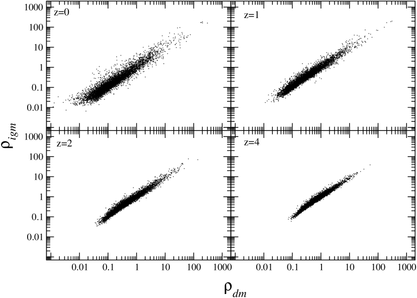
Figure 1: he relation between $\rho_{igm}(x)$ and $\rho_{dm}(x)$ for redshifts $z=0$, 1, 2 and 4. The data consists of $\simeq$ 7000 randomly drawn points from the simulation sample

As first evidence of the discrepancy between the IGM and dark matter, Fig. 1 gives the relation between $\rho_{dm}$ and $\rho_{igm}$ at redshifts 4, 2, 0.5 and 0. If $\rho_{dm}$ traces $\rho_{igm}$ point-by-point, we should have a tight correlation along the line $\rho_{dm}=\rho_{igm}$. However, Fig. 1 shows that although the relation $\rho_{dm}=\rho_{igm}$ is correct on average, the data points are significantly scattered around the line $\rho_{dm}=\rho_{igm}$ in the entire density range from $\rho_{dm}\sim$ 0.01 to $10^{2}$.

The scatter of the IGM vs. dark matter has been noted in SPH simulations (Gnedin & Hui 1998). They found that the IGM density contrast is significantly different from that of dark matter. They correctly pointed out that a pure N-body simulation would fail to reproduce the IGM distribution without mimicking the dynamical effect of the gas. They explain the scatter as a dynamical effect of gas pressure. The pressure of the IGM with temperature $\sim 10^{4}$ K is higher at higher redshifts, as the mean density of the gas is higher at earlier times. However, Fig. 1 shows that the scatter is smaller at higher redshifts. This would seem to contradict the gas pressure as an explanation for the scatter. On the other hand, the higher the nonlinearity, the higher the Reynolds number [eq.(6)], and the higher the discrepancy. Therefore, the gravitational nonlinear evolution of the IGM and dark matter system provides a plausible explanation of the scatter of Fig. 1.

4 One-point Statistics

4.1 One-point variables with the DWT decomposition

To calculate the one point distribution, we use the discrete wavelet transform (DWT). The scaling functions of the DWT analysis serve as the sampling window function. For the details of the mathematical properties of the DWT see Mallat (1989a,b); Meyer (1992); Daubechies (1992), and for cosmological applications see Fang & Thews (1998), Fang & Feng (2000).

Let us briefly introduce the DWT-decomposition for a random field. Consider a 1-D density fluctuation $\delta(x)$ on a spatial range from $x=0$ to $L$. We divide the space into $2^{j}$ segments labeled by $l=0,1,...2^{j}-1$ each of size $L/2^{j}$. The index $j$ is a positive integer and gives the length scale $L/2^{j}$. The larger the $j$ is, the smaller the length scale. Any reference to a property as a function of scale $j$ below must be interpreted as the property at length scale $L/2^{j}$. The index $l$ represents position and it corresponds to the spatial range $lL/2^{j}<x<(l+1)L/2^{j}$. Hence, the space $L$ is decomposed into cells $(j,l)$.

The discrete wavelet is constructed such that each cell $(j,l)$ supports a compact function, the scaling function $\phi_{j,l}(x)$, which satisfies the orthonormal relation

$$\int\phi_{j,l}(x)\phi_{j,l^{\prime}}(x)dx=\delta^{K}_{l,l^{\prime}},$$ (19)

where $\delta^{K}$ is Kronecker delta function. The scaling function $\phi_{j,l}(x)$ is a window function on scale $j$ centered around the segment $l$.

For a field $F(x)$, its mean in cell $(j,l)$ can be estimated by

$$F_{j,l}=\frac{\int_{0}^{L}F(x)\phi_{j,l}(x)dx}{\int_{0}^{L}\phi_{j,l}(x)dx}=\frac{1}{\int_{0}^{L}\phi_{j,l}(x)dx}\epsilon^{F}_{j,l},$$ (20)

where $\epsilon^{F}_{j,l}$ is called scaling function coefficient (SFC), given by

$$\epsilon^{F}_{j,l}=\int_{0}^{L}F(x)\phi_{j,l}(x)dx.$$ (21)

Thus, a 1-D field $F(x)$ can be decomposed into

$$F(x)=\sum_{l=0}^{2^{j}-1}\epsilon^{F}_{j,l}\phi_{j,l}(x)+O(\geq j).$$ (22)

The term $O(\geq j)$ in eq.(22) contains only the fluctuations of the field $F(x)$ on scales equal to and less than $L/2^{j}$. This term does not have any contribution to the window sampling on scale $j$. Thus, for a given $j$, the one-point variables $F_{j,l}$ or $\epsilon^{F}_{j,l}$ ($l=0,1...2^{j}-1$) give a complete description of the field $F(x)$ smoothed on scale $L/2^{j}$. As one-point variables the $\epsilon^{F}_{j,l}$ are similar to the measure given by count-in-cell technique. However, the orthonormality eq.(19) insures that the set of $F_{j,l}$ or $\epsilon^{F}_{j,l}$ do not cause false correlations. In the calculations below, we use the Daubechies 4 (D4) wavelet (Daubechies, 1992).

4.2 One-point variables of density fields

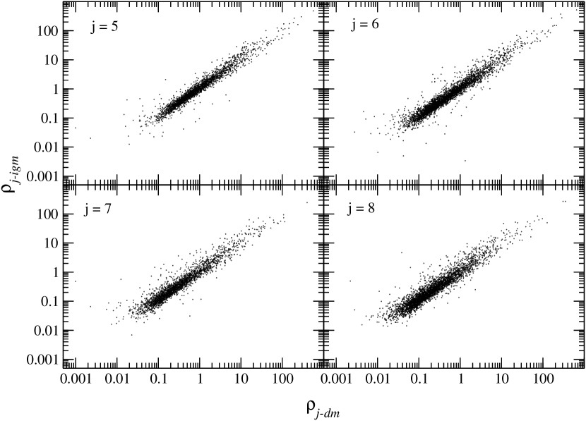
Figure 2: The relation between $\rho_{j,l-igm}$ and $\rho_{j,l-dm}$ on scales $j=5$, 6, 7 and 8, at redshifts $z=0$. The comoving scale corresponding to $j$ is $33/2^{j}$ h Mpc^-1. The data consists of $\simeq$ 7000 randomly drawn points from the simulation sample

We first calculate the one-point distributions of variables $\rho_{j,l-igm}$ and $\rho_{j,l-dm}$, which are the one-point variables given by eq.(20) replacing $F(x)$ by the density fields $\rho_{igm}(x)$ and $\rho_{dm}(x)$. We then plot in Fig. 2 $\rho_{j,l-igm}$ vs. $\rho_{j,l-dm}$ for $j=5$, 6, 7 and 8, corresponding to comoving length scales 1.03, 0.516, 0.258 and 0.129 h^-1 Mpc, respectively. Fig. 2 shows that the scatter around the line $\rho_{j,l-igm}=\rho_{j,l-dm}$ is little smaller for smaller $j$. That is, the discrepancy between the IGM and dark matter is smaller on larger scales. Nevertheless, the discrepancy is still substantial on scale $j=5$ or 1.03 h^-1 Mpc, which is larger than the Jeans length of the IGM.

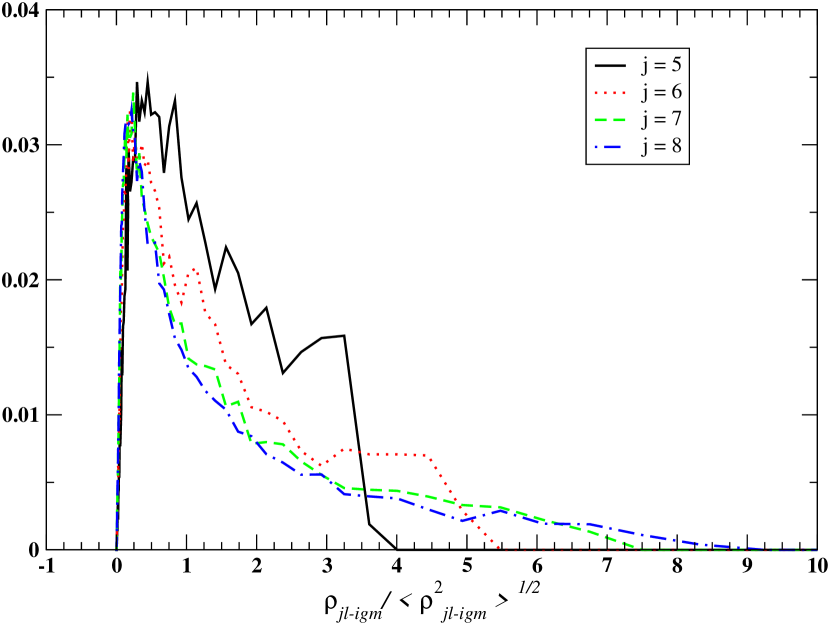
Figure 3: One-point distributions of the IGM density $\rho_{jl-igm}/\langle\rho^{2}_{jl-igm}\rangle^{1/2}$ at redshift $z=1$ and on scales $j=5$, 6, 7, 8. The comoving scale corresponding to $j$ is $33/2^{j}$ h^-1 Mpc.

When the “fair sample hypothesis” (Peebles 1980) holds, each set of 2^j ($l=0...2^{j-1}$) points form an ensemble from which the one-point distribution can be studied. Figure 3 gives the one-point distribution of $\rho_{j,l-igm}$ on scale $j=$ 5, 6, 7 and 8 at $z=1$. These distributions are generally non-Gaussian, having a longer tail at higher $j$, i.e., smaller scales. These distributions show significant $j$-dependence. The distribution at $j=8$ has a tail longer than 9 times the variance, while the tail of the distribution of $j=5$ is only about four times of the variance. We also see from Fig. 3 that the distribution has large change from $j=5$ to $j=6$, and from $j=6$ to $j=7$, but a smaller change from $j=7$ to $j=8$. This is because the scale $j=8$ is 0.129 h^-1 Mpc which is close to the Jeans length. On these scales the perturbations in the IGM field are weak. We show the redshift-evolution of the $\rho_{j,l-igm}$ one-point distributions in Fig. 4. The one-point distributions also undergoes significant redshift evolution. However, a long tail PDF is already pronounced at redshift $z=4$.

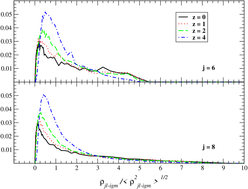
Figure 4: The redshift-dependence of the one-point distribution of the IGM density $\rho_{jl-igm}/\langle\rho^{2}_{jl-igm}\rangle^{1/2}$ on scales $j=6$ and 8 corresponding to comoving length scales 0.52 and 0.13 h^-1 Mpc

5 Statistical discrepancy between the IGM and dark matter

5.1 One-point distributions of velocity fields

To demonstrate the statistical discrepancy addressed in §2, we first analyze the one-point distributions of the 1-D velocity fields $v_{igm}({\bf x})$ and $v_{dm}({\bf x})$. For the linear solution $v_{igm}({\bf x})=v_{dm}({\bf x})$ [eq.(1)], we have $v_{j,l-igm}=v_{j,l-dm}$, which are the one-point variables given by eq.(20) replacing $F(x)$ by the velocity distribution. It is clear from Figure 5 that the one-point distributions of $v_{j,l-igm}$ and $v_{j,l-dm}$ at redshift $z=0$ are very different on all scales, $j=5$, 6, 7 and 8. This difference is smaller at higher redshift. At $z=4$, the one-point distributions of both $v_{j,l-igm}$ and $v_{j,l-dm}$ are basically the same on all scales.

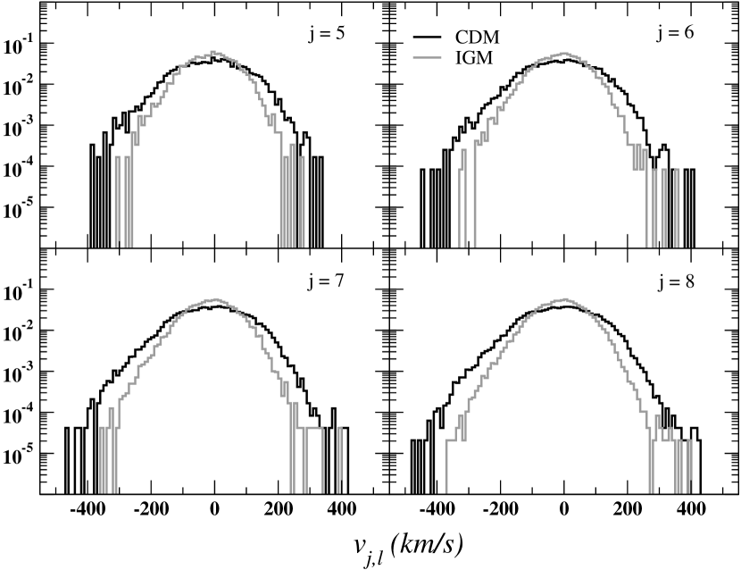
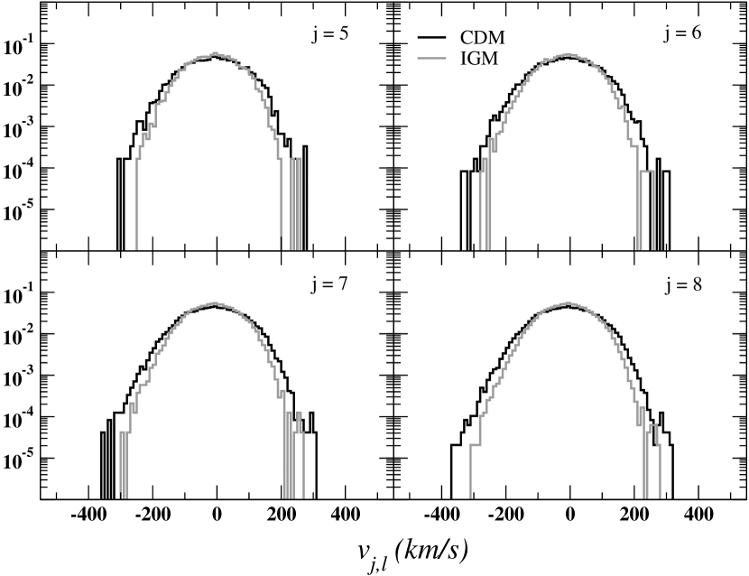
Figure 5: One-point distributions of the velocity fields of the IGM $v_{jl-igm}$ and dark matter $v_{jl-igm}$ on scales $j=5$, 6, 7, 8, and for redshifts $z=0$ (5a), 1 (5b), 2 (5c), 4 (5d).

The nature of the statistical difference between the $v_{j,l-igm}$ and $v_{j,l-dm}$ one-point distributions is not only quantitative, but also qualitative. The $v_{dm}({\bf x})$ one-point distributions are small deviations from a Gaussian PDF on all scales and all redshifts considered. This result is consistent with previous studies using N-body simulation samples (e.g. Yang et al 2001). On the other hand, the one-point distributions of the IGM velocity field shown in Fig. 5 are generally exponential at redshifts $z<2$. Even when the scale is as large as $j=5$ or $\sim 1$ h^-1 Mpc, the distribution of $v_{igm}({\bf x})$ is still exponential (Fig. 5a). This emphatically shows that the statistical discrepancy between the IGM and dark matter developed with dynamical evolution.

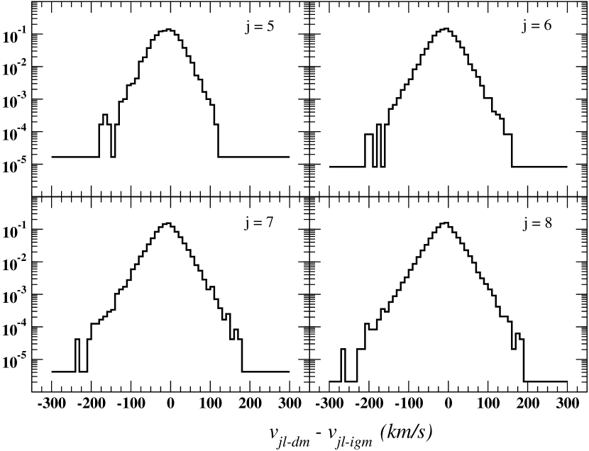
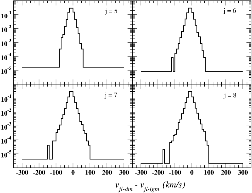
Figure 6: One-point distributions of the difference $v_{jl-dm}-v_{jl-igm}$ on scales $j=5$, 6, 7, 8, and for redshifts $z=0$ (6a), 1 (6b), 2 (6c), 4 (6d).

The dynamical equation (3) for the dark matter looks very similar to eq.(4) for the IGM. So why do the two one-point distributions have such different shapes? The reason is that the $\phi$ term of eq.(4) is truly an external force, as the gravity potential is independent of the IGM density and velocity, dependent only on the dark matter. Therefore, when its Reynolds number is large at lower redshifts, shocks or Burgers’ turbulence will develop in the IGM field due to the external driving force and the IGM velocity field will be highly non-Gaussian. On the other hand, the dark matter mass density in eq.(3) is not independent of the gravitational potential and there is no external driving force. Thus, when the gravity potential $\phi$ is Gaussian in weakly non-linear evolution, the dark matter velocity PDF will approximately be Gaussian too.

The statistical discrepancy of the velocity fields can also be seen with Fig. 6 which gives the one-point distribution of the difference $\bigtriangleup{\bf v}_{j,l}\equiv v_{j,l-dm}-v_{j,l-igm}$ on scales $j=5$, 6, 7 and 8, and redshifts 0, 1,2 and 4. These one-point distributions are non-Gaussian on all scales and redshift considered. Although the one-point distributions of $v_{dm}({\bf x})$ and $v_{igm}({\bf x})$ at redshift $z=4$ are not very different [Fig. 5d], their differences [Fig. 6d] are highly non-Gaussian. Therefore, the discrepancy between $v_{j,l-dm}$ and $v_{j,l-igm}$ is not due to noise, but arises from the non-linear evolution of the IGM fluid.

5.2 One-point distributions of density fields

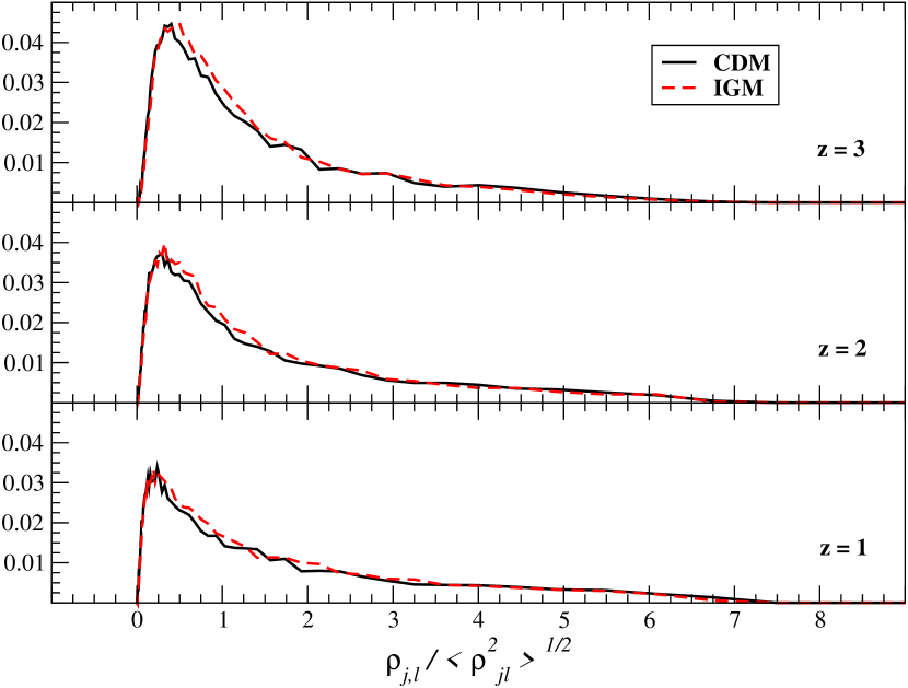
Figure 7: One-point distributions of the IGM density $\rho_{jl-igm}/\langle\rho^{2}_{jl-igm}\rangle^{1/2}$ and dark matter $\rho_{jl-dm}/\langle\rho^{2}_{jl-dm}\rangle^{1/2}$ at redshift $z=1$, 2 and 3 and on scales $j=7$, or comoving length scale 0.26 h^-1 Mpc.

Figure 7 presents the one-point distributions for $\rho_{j,l-igm}$ and $\rho_{j,l-dm}$ on scale $j=7$ and redshifts $z=1$, 2 and 3. The horizontal axes are the variance-normalized densities, $\rho_{j,l-igm}/\langle\rho^{2}_{j,l-igm}\rangle^{1/2}$ and $\rho_{j,l-igm}/\langle\rho^{2}_{j,l-dm}\rangle^{1/2}$. Unlike the velocity fields, both the IGM and dark matter show highly non-Gaussian behavior even at redshift $z=3$. Additionally, the two curves in Fig. 7 are not significantly different. That is, the mass density one-point distribution is not as sensitive to the statistical discrepancy as the velocity one-point distribution. This is probably because the statistical discrepancy between a “passive substance” and underlying field is significant only for non-conserved quantities (temperature, velocity etc.) (Shraiman & Siggia 2001.) Nevertheless, one can see from Fig. 7 that the IGM distributions are always a little higher than the corresponding distribution for the dark matter at the range around $\rho_{j,l-igm}/\langle\rho^{2}_{j,l-igm}\rangle^{1/2}\simeq 1$. This indicates that the tail of the IGM one-point distribution should be shorter than that of dark matter. Therefore, we can expect that the high order moments of the one-point distributions will more clearly show the discrepancy between the IGM and dark matter.

In this paper, we use only the second order moment. The correlation between $\rho_{j,l-igm}$ and $\rho_{j,l-dm}$ can be measured with the ratio $I_{dm}$, $I_{igm}$ [eqs.(10), (11)], or $I$ [eq.(12)]. Using the DWT one-point variables $\rho_{j,l-igm}$ and $\rho_{j,l-dm}$, we can redefine, respectively, the ratios $I_{dm}$ and $I_{igm}$ as

$$I_{j,-dm}=\frac{[\langle[\rho_{j,l-dm}-\rho_{j,l-igm}]^{2}\rangle^{1/2}}{\langle\rho_{j,l-dm}^{2}\rangle^{1/2}}$$ (23)

$$I_{j,-igm}=\frac{[\langle[\rho_{j,l-dm}-\rho_{j,l-igm}]^{2}\rangle^{1/2}}{\langle\rho_{j,l-igm}^{2}\rangle^{1/2}}$$ (24)

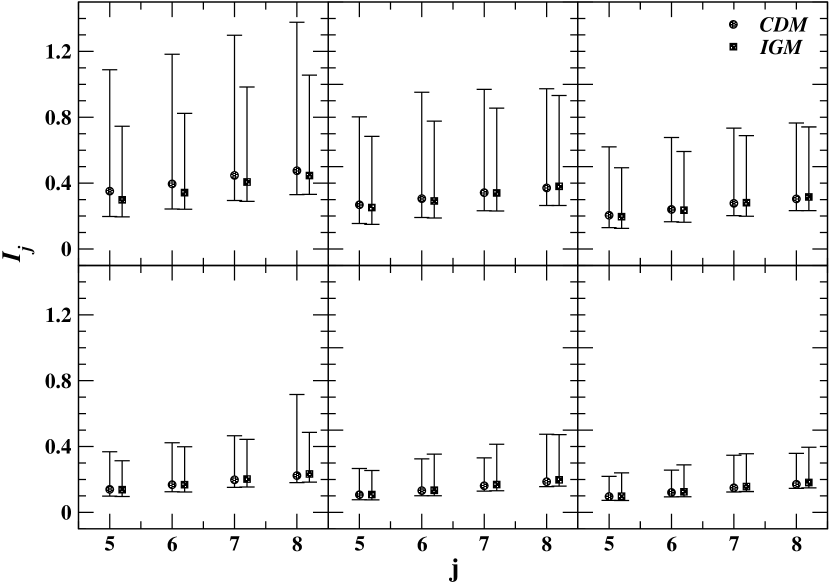
Figure 8: The ratio $I_{j}$ at redshifts $z=0$, top left panel, to redhsifts 0.5, 1, 2, 3, 4, (moving left to right) and on scales $j=5$, 6, 7, 8, which corresponds to the comoving scales $33/2^{j}$ h^-1 Mpc.

From the one-point distributions of Fig. 7, we have $\langle\rho_{j,l-dm}^{2}\rangle\simeq\langle\rho_{j,l-igm}^{2}\rangle$. Thus, if $\rho_{j,l-igm}$ perfectly traces $\rho_{j,l-dm}$, we have correlation $\langle\rho_{j,l-igm}\rho_{j,l-dm}\rangle\simeq\langle\rho^{2}_{j,l-igm}\rangle\simeq\langle\rho^{2}_{j,l-dm}\rangle$, and therefore, $I_{j,-dm}\simeq I_{j,-igm}\simeq 0$. If $\rho_{j,l-igm}$ is fully independent of $\rho_{j,l-dm}$, we have $I_{j,-dm}\simeq I_{j,-igm}\simeq\sqrt{2}$.

Figure 8 plots $I_{j,-dm}$ and $I_{j,-igm}$ for $z=0$, 0,5, 1, 2, 3 and 4 on scales $j=5$, 6, 7 and 8. The error bars are the 67% confidence level of the 500 1-D samples. Figure 8 shows that $I_{j}$ is always larger than 0, equal to $\sim 0.1-0.2$ at redshift $\geq 2$, and $\sim 0.3-0.6$ at redshift $<2$, and weakly dependent on scales. That is, the cross correlation at redshift $<$ 2 is

$$\frac{\langle\rho_{j,l-igm}\rho_{j,l-dm}\rangle}{\langle\rho^{2}_{j,l-igm}\rangle},{\rm\ \ \ or\ \ \ }\frac{\langle\rho_{j,l-igm}\rho_{j,l-dm}\rangle}{\langle\rho^{2}_{j,l-dm}\rangle}\simeq 0.70-85$$ (25)

Therefore, the IGM is not a perfect tracer at low redshift and on scales larger than the Jeans length. These results indicate that 15 -30% of the two density fields are off-correlated. This is consistent with the analysis in §2.2.

5.3 One-point distribution of $\bigtriangleup\delta({\bf x})$

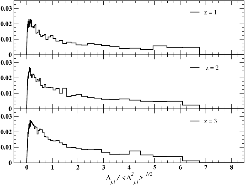
Figure 9: One-point distributions of the difference $\bigtriangleup_{j,l}/\langle\bigtriangleup^{2}_{j,l}\rangle^{1/2}>0$ for redshift $z=1$, 2 and 3, and on scale $j=7$, or 0.26 h^-1 Mpc.

The DWT one-point variable for the density difference $\bigtriangleup\delta(x)$ [eq.(2)] is given by

$$\bigtriangleup_{j,l}=\int\bigtriangleup\delta(x)\phi_{j,l}(x)dx.$$ (26)

Since $\phi_{j,l}(x)$ is localized in cell $(j,l)$, the integral $\int\phi_{j,l}\phi_{j,l^{\prime}}\phi_{j,l^{\prime\prime}}dx$ is generally non-zero only for $l=l^{\prime}=l^{\prime\prime}$ (for Haar wavelet, this is exactly true. For other wavelets, the integral with $l\neq l^{\prime},\ l^{\prime\prime}$ is much less than that of $l=l^{\prime}=l^{\prime\prime}$). Thus, for two fields $A(x)$ and $B(x)$, we have $\int A(x)B(x)\psi_{jl}(x)dx\simeq g_{j}\epsilon^{A}_{jl}\epsilon^{B}_{jl}$, where $\epsilon^{A}_{jl}$ and $\epsilon^{B}_{jl}$ are the WFCs of $A(x)$ and $B(x)$. The factor $g_{j}$ is

$$g_{j}=\int\psi^{3}_{jl}(x)dx.$$ (27)

which is the factor $g_{W}$ used in eq.(16).

With $\bigtriangleup_{j,l}$, eq. (15) can be rewritten as

$$\frac{d\bigtriangleup_{j,l}}{dt}=-\frac{1}{a}\lambda_{j}\bigtriangleup_{j,l}+\frac{1}{a}\eta_{j},$$ (28)

where

$$\eta_{j}=\int dx^{\prime}\psi_{jl}(x^{\prime})(\nabla\cdot\bigtriangleup{\bf v}(x)).$$ (29)

and

$$\lambda_{j}=g_{j}\int x^{\prime}\psi_{jl}(x^{\prime})(\nabla\cdot{\bf v}_{dm}).$$ (30)

As discussed in §2.3, the PDF of $\bigtriangleup_{j,l}$ should be long tailed.

The normalized one-point distributions of $\bigtriangleup_{j,l}/\langle\bigtriangleup^{2}_{j,l}\rangle^{1/2}$ for $j=7$ and redshifts 1,2, and 3 are plotted in Fig. 9. All the tails of the distributions are remarkably long. They have 6 $\sigma$ events at $z\leq 3$ with probability $\sim$ 0.005, while for a Gaussian field, the probability of 6-$\sigma$ is $<10^{-8}$. This shows again that the statistical discrepancy between the IGM and dark matter is not due to processes like Jeans diffusion or Gaussian noise. Fitting the tails with a power law $(\bigtriangleup_{j,l}/\langle\bigtriangleup^{2}_{j,l}\rangle^{1/2})^{-\beta}$, we have $\beta<1$. This result is consistent with the dynamical eq.(28).

6 Conclusion

Using the dynamical equations governing the IGM, we have shown that the decoupling of important statistical properties of the gas component from the underlying dark matter field on scales larger than the Jeans length is inevitable. The one-point distribution of the IGM peculiar velocity field is found to be substantially different from that of dark matter at redshift $\leq 2$. Although the one-point distribution of the IGM mass density field shows only a little deviation from that of the dark matter, the density fields of the IGM and dark matter are not point-by-point correlated, and a significant part of the two fields is off-correlated on all redshifts $z\leq 4$.

It is difficult to explain the discrepancy as an effect of Jeans smoothing, as the discrepancy is still evident even when the fields are smoothed on scales $>1$ h^-1 Mpc ($j=5$). This is much larger than the Jeans length of the IGM with temperature $\sim 10^{4}$ K at the mean density. The Jeans length of the IGM may be $>1$ h^-1 Mpc in an area with high temperatures $\simeq 10^{7}$ K, but not one with high density. Yet, even in this case Jeans smoothing does not adequately explain the statistical discrepancy, because the difference between the density distributions of the IGM and dark matter is highly non-Gaussian.

The decoupling of the IGM from the dark matter mass field is important for problems in large scale structure formation. Some observations have already implied that the IGM and dark matter have decoupled. For instance, X-ray measurements find no evidence for the baryon fraction of clusters to be equal to the universal value from cosmological nucleosynthesis (White & Fabian 1995; David 1997; Ettori, Fabian & White 1997; White, Jones & Forman 1997; Ettori & Fabian, 1999). This result violates the similarity the IGM and dark matter if typical galaxy clusters formed from linear fields on scales of a few ten (comoving) Mpc, which is much larger than the Jeans length of the IGM. Moreover, the X-ray observed luminosity-temperature relation for groups and clusters is found to be inconsistent with the prediction given by the similarity between the IGM and dark matter. The high entropy floor observed in nearby groups and low mass clusters directly violates the dynamical self-similar scaling (Ponman, Cannon, & Navarro 1999; Lloyd-Davies, Ponman, & Cannon 2000). Although, at present we cannot attribute all these discrepancies to the decoupling shown in this paper, we now understand that the dynamics of the IGM and dark matter fields will lead to a qualitatively different evolution of those fields. While we did not consider stellar formation and its feedback to the IGM in our present simulations, we believe that the statistical discrepancy will still be a common feature even when these effects are considered because the reason for discrepancy we have uncovered arises from the nonlinear evolution of the random fields of the IGM and dark matter.

Finally, we should mention the effect of the size of the simulated sample. Since the simulation box is only 25 h^-1 Mpc, the use of the fair sample hypothesis may not be appropriate when considering perturbations on scales larger than this. We can estimate the effect of these larger perturbations by adding long-wavelength modes (Tormen & Bertscinger 1996). Since the IGM and dark matter fields are linear or quasi-linear on scales larger than 25 h^-1 Mpc, the effect of long-wavelength perturbations can be analyzed by adding a displacement to each particle in the simulation box. The displacement is given by the linear field or Zeldovich approximation of the field consisting of modes on scales larger than 25 h^-1 Mpc. As was discussed in §1, there is no discrepancy between the IGM and dark matter in the linear or quasi-linear regime. Thus, the displacement for the IGM is the same as that of the dark matter meaning that long wavelength modes are not a source of the discrepancy between the IGM and dark matter.

Appendix A Hydrodynamic equations for dark matter fields

Let us consider a flat universe having cosmic scale factor $a(t)\propto t^{2/3}$ and dominated by dark matter. In a hydrodynamic description, the dark matter is described by a mass density field $\rho_{dm}({\bf x},t)$ and a peculiar velocity field ${\bf v}_{dm}({\bf x},t)$, where ${\bf x}$ is the comoving coordinate. The field is described by the equations of continuity, momentum and gravitational potential as (Wasserman 1978)

$$\frac{\partial\delta_{dm}}{\partial t}+\frac{1}{a}\nabla\cdot(1+\delta_{dm}){\bf v}_{dm}=0$$ (A1)

$$\frac{\partial a{\bf v}_{dm}}{\partial t}+({\bf v}_{dm}\cdot\nabla){\bf v}_{dm}=-\nabla\phi$$ (A2)

$$\nabla^{2}\phi=4\pi Ga^{2}\bar{\rho}_{dm}\delta_{dm}.$$ (A3)

The mean density is $\bar{\rho}_{dm}(t)=1/6\pi Gt^{2}\propto a^{-3}$. The gravitational potential $\phi$ is zero (or constant) when the density perturbation $\delta_{dm}=0$. The operator $\nabla$ acts on the comoving coordinate ${\bf x}$.

For growth modes in the perturbations, velocity is irrotational. We can then define a velocity potential by

$${\bf v}_{dm}=-\frac{1}{a}\nabla\varphi_{dm}.$$ (A4)

The momentum equation (A2) can then be rewritten as

$$\frac{\partial\varphi_{dm}}{\partial t}-\frac{1}{2a^{2}}(\nabla\varphi_{dm})^{2}=\phi.$$ (A5)

This is the Bernoulli equation.

Appendix B Hydrodynamic equations for the IGM

As usual, the IGM is assumed to be ideal fluid with polytropic index $\gamma=5/3$. The hydrodynamic equations of the IGM are (Peebles 1980)

$$\frac{\partial\delta_{igm}}{\partial t}+\frac{1}{a}\nabla\cdot(1+\delta_{igm}){\bf v}_{igm}=0$$ (B1)

$$\frac{\partial a{\bf v}_{igm}}{\partial t}+({\bf v}_{igm}\cdot\nabla){\bf v}_{igm}=-\frac{1}{\rho_{igm}}\nabla p-\nabla\phi$$ (B2)

$$\frac{\partial{\cal E}}{\partial t}+5\frac{\dot{a}}{a}{\cal E}+\frac{1}{a}\nabla\cdot({\cal E}{\bf v}_{igm})=-\frac{1}{a}\nabla\cdot(p{\bf v}_{igm})-\frac{1}{a}\rho_{igm}{\bf v}_{igm}\cdot\nabla\phi-\Lambda_{rad},$$ (B3)

where $\rho_{igm}$, ${\bf v}_{igm}$, ${\cal E}$ and $p$ are, respectively, the mass density, peculiar velocity, energy density and pressure of the IGM. The term $\Lambda_{rad}$ in Eq.(2) is given by the radiative heating-cooling of the baryonic gas per unit volume. The gravitational potential $\phi$ in eqs.(B2) and (B3) can still be given by eq. (A3). That is, the gravity of the IGM is negligible. The evolution of the IGM mass field $\rho_{igm}({\bf x},t)$ is governed by the gravity of dark matter only.

The hydrodynamic equations for the IGM, eqs.(B1)-(B3) can be written in the form of conservation laws for mass, momentum, and energy in a comoving volume as

$$\frac{\partial a^{3}\rho}{\partial t}+\frac{1}{a}\frac{\partial}{\partial x_{i}}(a^{3}\rho v_{i})=0,$$ (B4)

$$\frac{\partial a^{3}\rho v_{i}}{\partial t}+\frac{1}{a}\frac{\partial}{\partial x_{j}}(a^{3}\rho v_{i}v_{j}+a^{3}p\delta_{ij})=-\dot{a}a^{2}\rho v_{i}-a^{2}\rho\nabla\phi$$ (B5)

$$\frac{\partial a^{3}{\cal E}}{\partial t}+\frac{1}{a}\frac{\partial}{\partial x_{i}}[a^{3}({\cal E}+p)v_{i}]=-2\dot{a}a^{2}{\cal E}-a^{2}\rho{\bf v}\cdot\nabla\phi-a^{3}\Lambda_{rad}.$$ (B6)

In eqs.(B4)-(B6), we dropped the subscript $igm$ for simplicity.

To sketch the gravitational clustering of the IGM, it is not necessary to consider the details of heating and cooling. Thermal processes are generally highly localized, and therefore, it is reasonable to describe all thermal processes by a polytropic relation $p({\bf x},t)\propto\rho_{igm}^{\gamma}({\bf x},t)$. Thus eq.(B2) becomes

$$\frac{\partial a{\bf v}_{igm}}{\partial t}+({\bf v}_{igm}\cdot\nabla){\bf v}_{igm}=-\frac{\gamma k_{B}T}{\mu m_{p}}\frac{\nabla\delta_{igm}}{(1+\delta_{igm})}-\nabla\phi$$ (B7)

where the parameter $\mu$ is the mean molecular weight of the IGM particles, and $m_{p}$ the proton mass. Here, we don’t need the energy equation and the IGM temperature evolves as $T\propto\rho^{\gamma-1}$, or $T=T_{0}(1+\delta_{igm})^{\gamma-1}$.

Eq.(B7) differs from eq.(A2) only by the temperature-dependent term. If we treat this term in the linear approximation, we have

$$\frac{\partial\varphi_{igm}}{\partial t}-\frac{1}{2a^{2}}(\nabla\varphi_{igm})^{2}-\frac{\nu}{a^{2}}\nabla^{2}\varphi_{igm}=\phi,$$ (B8)

where $\varphi_{igm}$ is the velocity potential for the IGM field defined by

$${\bf v}_{igm}=-\frac{1}{a}\nabla\varphi_{igm}.$$ (B9)

The coefficient $\nu$ is given by

$$\nu=\frac{\gamma k_{B}T_{0}}{\mu m_{p}(d\ln D(t)/dt)},$$ (B10)

where $D(t)$ describes the linear growth behavior. The term with $\nu$ in eq.(B8) acts like a viscosity (due to thermal diffusion) characterized by the Jeans length $k_{J}^{2}=(a^{2}/t^{2})(\nu m_{p}/\gamma k_{B}T_{0})$.

The unperturbed solutions of the density and velocity fields of both dark and baryonic matter are $\bar{\rho}_{b}=(\Omega_{b}/\Omega_{dm})\bar{\rho}\propto a^{-3}$, and ${\bf v}_{b}={\bf v}=0$, where $\Omega_{b}$ and $\Omega_{dm}$ are, respectively, the density parameters of the IGM and dark matter. Therefore, the linearlization of eqs. (B1) and (B7) yields

$$\frac{\partial\delta_{igm}}{\partial t}+\frac{1}{a}\nabla\cdot{\bf v}_{igm}=0$$ (B11)

$$\frac{\partial a{\bf v}_{igm}}{\partial t}=-\frac{\gamma k_{B}\overline{T}}{\mu m_{p}}\nabla\delta_{igm}-\nabla\phi$$ (B12)

where the mean temperature $\overline{T}\propto\overline{\rho_{b}}^{\gamma-1}\propto a^{-3(\gamma-1)}$. In Fourier space, we have

$$\frac{\partial^{2}\delta_{igm}({\bf k},t)}{\partial t^{2}}+2\frac{\dot{a}}{a}\frac{\partial\delta_{igm}({\bf k},t)}{\partial t}+\frac{1}{t^{2}}\frac{k^{2}}{k_{J}^{2}}\delta_{igm}({\bf k},t)=4\pi G\bar{\rho}\delta_{dm}({\bf k},t)$$ (B13)

$$\frac{\partial\upsilon_{igm}({\bf k},t)}{\partial t}+\frac{\dot{a}}{a}\upsilon_{igm}({\bf k},t)=-\frac{1}{t^{2}a}\frac{1}{k^{2}_{J}}\delta_{igm}({\bf k},t)+\frac{4\pi G\bar{\rho}a}{k^{2}}\delta_{dm}({\bf k},t),$$ (B14)

where ${\bf v}_{igm}({\bf k},t)=i{\bf k}\upsilon_{igm}({\bf k},t)$, and the Jeans wavenumber $k^{2}_{J}=(a^{2}/t^{2})(\mu m_{p}/\gamma k_{b}\overline{T})\propto a^{3\gamma-4}$. If $\gamma=4/3$, $k_{J}$ is time-independent.

In solving equations (B13) and (B14), we consider only the growth mode of the perturbation of dark matter, i.e. $\delta({\bf k},t)\propto a$. In the case of $\gamma=4/3$, the solution of eqs.(B13) and (B14) is (Bi, Börner, Chu 1993)

$$\delta_{igm}({\bf k},t)=\frac{\delta_{bm}({\bf k},t)}{1+3k^{2}/2k_{J}^{2}}+c_{1}t^{-(1+\epsilon)/6}+c_{2}t^{-(1-\epsilon)/6}$$ (B15)

where $\epsilon=(1-4k^{2}/9k_{J}^{2})^{1/2}$, and constants $c_{1}$ and $c_{2}$ depend on the initial condition $\delta_{igm}({\bf k},0)$ and $\upsilon_{igm}({\bf k},0)$. Therefore, regardless the initial condition of IGM, after a long evolution we have

$$\delta_{igm}({\bf k},t)=\delta_{dm}({\bf k},t),\hskip 14.22636pt{\bf v}_{igm}({\bf k},t)={\bf v}_{dm}({\bf k},t),\hskip 28.45274pt{\rm if}\ k\ll k_{J}.$$ (B16)

These solutions mean that the initial conditions of the IGM are unimportant. The IGM will, in the end, follow the same trajectory as the dark matter on scales larger than the Jeans length.

The solutions of linear equations (B11) and (B12) have also been found by using assumptions of the IGM thermal processes other than that used in eqs.(B13) and (B14) (e.g. Nusser 2000, Matarrese & Mohayee 2002). A common feature of these solutions is

$$\delta_{b}({\bf k},t)=(1+{\rm decaying\ terms})\delta({\bf k},t)+{\rm decaying\ terms},\hskip 28.45274pt{\rm if}\ k\ll k_{J}.$$ (B17)

The initial conditions of the IGM field affects only the decaying terms, and therefore, the linear solutions eq.(B16) hold in general regardless specific assumptions of IGM thermal processes.

Appendix C PDF of $\bigtriangleup_{j,l}$ in eq.(27)

Using $d\tau=dt/a$, eq. (28) can be rewritten as

$$\frac{d\bigtriangleup_{j,l}}{d\tau}=-\lambda_{j}\bigtriangleup_{j,l}+\eta_{j}.$$ (C1)

If the stochastic forces $\lambda_{j}$ and $\eta_{j}$ are Gaussian, then

$$\langle\lambda_{j}\rangle = \overline{\lambda}_{j}$$ (C2)

$$\langle[\lambda_{j}(\tau)-\overline{\lambda}_{j}][\lambda_{j}(\tau^{\prime})-\overline{\lambda}_{j}]\rangle = 2D_{\lambda,j}\delta(\tau-\tau^{\prime})$$

$$\langle\eta_{j}\rangle = 0$$

$$\langle\eta_{j}(\tau)\eta_{j}(\tau^{\prime})\rangle = =2D_{\eta,j}\delta(\tau-\tau^{\prime})$$

The Fokker-Planck equation corresponding to eq.(C1) is (Venkataramani et al. 1996)

$$\frac{\partial}{\partial\tau}P(\bigtriangleup_{j,l},\tau)=-\frac{\partial}{\partial\bigtriangleup_{j,l}}j(\bigtriangleup_{j,l},\tau)$$ (C3)

where $P(\bigtriangleup_{j,l},\tau)$ is the PDF of $\bigtriangleup_{j,l}$, and the flux $j(\bigtriangleup_{j,l},\tau)$ is given by

$$j(\bigtriangleup_{j,l},\tau)=(-\overline{\lambda}_{j}+D_{\lambda,j})\bigtriangleup_{j,l}P(\bigtriangleup_{j,l},\tau)-\frac{\partial}{\partial\bigtriangleup_{j,l}}[D_{\lambda,j}|\bigtriangleup_{j,l}|^{2}+D_{\eta,j}]P(\bigtriangleup_{j,l},\tau).$$ (C4)

For stationary solution, $\partial P(\bigtriangleup_{j,l},\tau)/\partial\tau=0$, and therefore, $\partial j(\bigtriangleup_{j,l},\tau)/\partial\bigtriangleup_{j,l}=0$. We have $j(\bigtriangleup_{j,l})=$ const. However, when $\bigtriangleup_{j,l}$ is very large, we should have $j(\bigtriangleup_{j,l})=0$, and therefore $j(\delta^{R}_{D})=0$. Thus, we have equation as

$$(-\overline{\lambda}_{j}+D_{\lambda,j})\bigtriangleup_{j,l}P(\bigtriangleup_{j,l},\tau)-\frac{\partial}{\partial\bigtriangleup_{j,l}}[D_{\lambda,j}|\bigtriangleup_{j,l}|^{2}+D_{\eta,j}]P(\bigtriangleup_{j,l},\tau)=0$$ (C5)

The solution of eq.(C5) is

$$P(\bigtriangleup_{j,l})=C(D_{\lambda,j}|\bigtriangleup_{j,l}|^{2}+D_{\eta,j})^{-\overline{\lambda}_{j}/2D_{\lambda,j}-1/2}$$ (C6)

where $C$ is a normalization constant. Th PDF is then

$$P(\bigtriangleup_{j,l})\propto\left\{\begin{array}[]{ll}{\rm const}&\mbox{$0<\bigtriangleup_{j,l}|\ll s$ }\\ (\bigtriangleup_{j,l})^{-\beta}&\mbox{$|\bigtriangleup_{j,l}|\gg s$}\\ \end{array}\right.$$ (C7)

where

$$s=\frac{D_{\eta,j}}{D_{\lambda,j}},$$ (C8)

and

$$\beta=\frac{\overline{\lambda}_{j}}{D_{\lambda,j}}+1.$$ (C9)

References

- (1)
- (2) Balsara, D. & Shu, C.-W., 2000, J. Comput. Phys., 160, 405
- (3)
- (4) Barabási, A.L. & Stanley, H.E. 1995, Fractal Concepts in Surface Growth, (Cambridge Univ. Press)
- (5)
- (6) Berera, A. & Fang, L.Z. 1994, Phys. Rev. Lett., 72, 458
- (7)
- (8) Bi, H., Börner, G. & Chu, Y.Q. 1992, A&A, 266, 1.
- (9)
- (10) Borve, S., Omang, M., & Trulsen, J. 2001, ApJ, 561, 82
- (11)
- (12) Buchert,T., Domínguez,A., Pérez-Mercader, J., 1999, A&A,349,3432.
- (13)
- (14) Carrillo, J.A., Gamba, I. M., Majorana, A.. Shu, C.W. 2003, J. of Comput. Physics, 184, 498
- (15)
- (16) Cen, R.Y., 1992, ApJS, 78, 341
- (17)
- (18) Coles, P., Spencer, K., 2003, MNRAS, 342, 176.
- (19)
- (20) Daubechies I. 1992, Ten Lectures on Wavelets (Philadelphia: SIAM)
- (21)
- (22) David, L.P. 1997, ApJ, 484, 11
- (23)
- (24) Eisenstein,D.J. & Hu, W., 1999, ApJ, 511, 5
- (25)
- (26) Ettori, S.; Fabian, A. C. 1999, MNRAS, 305, 834
- (27)
- (28) Ettori, S. Fabian, A. C. & White, D. A. 1997, MNRAS, 289, 787
- (29)
- (30) Fang, L.Z., Bi, H.G., Xiang, S.P & Börner, G. 1993, ApJ, 413, 477
- (31)
- (32) Fang, L.Z. & Feng, L.L. 2000, ApJ, 539, 5
- (33)
- (34) Fang, L.Z. & Thews, R. 1998, Wavelet in Physics (Singapore: World Scientific)
- (35)
- (36) Fedkiw, R. P., Guillermo, S. & Shu, C.-W 2003, J. of Computational Physics, 185, 309
- (37)
- (38) Feng, L.L. Pando, J. & Fang, L.Z. 2003, ApJ, 587, 487
- (39)
- (40) Feng, L.L., Shu, C.-W., & Zhang, M. 2004, ApJ, in press.
- (41)
- (42) Gnedin, N. & Hui, L. 1998, ApJ, 296, 44.
- (43)
- (44) Godlewski, E., & Raviart, P.A. 1996, Numerical approximation of hyperbolic systems of conservation laws, (Springer)
- (45)
- (46) Graham, R., Höhnerbach, M. & Schenzle, A. 1982, Phys. Rev. Lett., 48, 1396
- (47)
- (48) Grasso F., & Pirozzoli, S., 2000a, Theor. Comp. Fluid Dyn., 13, 421
- (49)
- (50) Grasso, F., & Pirozzoli, S., 2000b, Phys. Fluids, 12, 205
- (51)
- (52) Harten, J. Comp. Phys. 49, 357, 1983
- (53)
- (54) Harten, A., Osher, S., Engquist, B., & Chakravarthy, S. 1987, Applied Numerical Mathematics, 2, 347
- (55)
- (56) He, P., Feng, L.L. and Fang, L.Z. 2004, ApJ, in press
- (57)
- (58) Jamkhedkar, P., Feng, L.L., Zheng, W., Kirkman, D., Tytler, D., and Fang, L.Z. 2003, MNRAS, 343, 1110
- (59)
- (60) Jamkhedkar, P., Zhan, H. and Fang, L.Z. 2000, ApJ, 543, L1
- (61)
- (62) Jiang, G. & Shu, C.W., 1996, J. Comput. Phys. 126, 202
- (63)
- (64) Jiang, G. & Wu, C.-C. 1999, J. Comput. Phys., 150, 561
- (65)
- (66) Jones, B.T., 1999, MNRAS, 307, 376
- (67)
- (68) Kaiser, N. 1986, MNRAS, 222, 323
- (69)
- (70) Kardar, M, Parisi, G & Zhang, Y.C. 1986, Phys. Rev. Lett. 56, 342.
- (71)
- (72) Kraichnan, R. H. 1968, Phys. of Fluids, 11, 265
- (73)
- (74) Kraichnan, R. H. 1994, Phys. Rev. Lett., 72, 1016
- (75)
- (76) Lässig, M. 2000, Phys. Rev. Lett. 84, 2618
- (77)
- (78) Liang, S. & Chen, H., 1999, AIAA J., 37, 1010
- (79)
- (80) Lui, X.-D, Osher, S. & Chan, T. 1994, J. Comput. Phys., 115, 200.
- (81)
- (82) Lloyd-Davies, E. J. Ponman, T. J. & Cannon, D. B. 2000, MNRAS, 315, 689
- (83)
- (84) Ma,C.P., & Bertschinger, E., 2003, Phys Rev D submitted, astro-ph/0311049
- (85)
- (86) Mallat, S.G. 1989a, IEEE Trans., 11, 674
- (87)
- (88) Mallat, S.G. 1989b, Trans. Am. Math. Soc., 315, 69
- (89)
- (90) Matarrese, S. & Mohayaee, R. 2002, MNRAS, 329, 37
- (91)
- (92) Meyer, Y. 1992, Wavelets and Operators (New York: Cambridge Press)
- (93)
- (94) Nakao, H. 1998, Phys. Rev. E58, 1591
- (95)
- (96) Nusser, A., 2000, MNRAS, 317, 902.
- (97)
- (98) Nusser, A. & Haehnet, M. 1999, MNRAS, 303, 179
- (99)
- (100) Omang, M., Borve, S. & Trulsen, J. 2003, Comput. Fluid Dynamics 12, 32.
- (101)
- (102) Pando, J., Feng, L.L., Jamkhedkar, P., Zheng, W., Kirkman, D., Tytler, D. and Fang, L.Z. 2002, ApJ, 574, 575
- (103)
- (104) Peebles, P. J. E., 1980, The large scale structure of the universe, (Princeton University Press)
- (105)
- (106) Platt, N., Hammel, S.M. & Heagy, J.F. 1994, Phys. Rev. Lett., 72, 3498
- (107)
- (108) Ponman, T. J. Cannon, D. B. & Navarro, J. F. 1999, Nature, 397, 135
- (109)
- (110) Ryu, D., Kang, H., Hallman, E., & Jones, T.W. 2003, ApJ, 593, 599
- (111)
- (112) Shandarin, S.F. & Zel’dovich, Ya.B. 1984, Phys.. Rev. Lett., 52, 1448
- (113)
- (114) Shi, J., Zhang, Y.T. & Shu, C.W., 2003, J. of Comput. Physics, 186, 690
- (115)
- (116) Shraiman B.I. & Siggia, E.D. 2000, Nature, 405, 639
- (117)
- (118) Shu, C.W. 1998, in Advanced Numerical Approximation of Nonlinear Hyperbolic Equations, Ed. A. Quarteroni, Lecture Notes in Mathematics, (Springer), 1697, 325
- (119)
- (120) Shu, C.W. 1999, in High-Order Methods for Computational Physics, Eds. T.J. Barth and H. Deconinck, Lecture Notes in Computational Science and Engineering, (Springer), volume 9, 439
- (121)
- (122) Shu, C.W. 2003, Inter. J. of Computational Fluid Dynamics, 17, 107
- (123)
- (124) Tormen, G. & Bertschinger, E. 1996, ApJ, 472, 14
- (125)
- (126) Venkataramani, S.C., Antonsen,jr. T.M., Ott, E., & Sommerer, J.C., 1996, Physica D, 96, 66
- (127)
- (128) Walker, T.P., Steigman, G., Schramm, D.N., Olive, K.A. & Kang, H.S., 1991, ApJ376, 51
- (129)
- (130) Wasserman, I., 1978 ApJ, 224, 337
- (131)
- (132) White, D. A.& Fabian, A.C. 1995, MNRAS, 273, 72
- (133)
- (134) White, D. A.; Jones, C.; Forman, W. 1997, MNRAS, 292, 419
- (135)
- (136) Yang, H.X., Feng, L.L., Y.Q. Chu & Fang, L.Z. 2001, ApJ, 560, 549
- (137)
- (138) Zanna, L. Del, Velli, M. & Londrillo, P., 1998, A&A, 330, L13
- (139)
- (140) Zeldovich, Y.B., Ruzmaikin, A.A. & Sokoloff, D.D., 1990, The Almighty Chance, (World Scientific)
- (141)
- (142) Zhan, H. & Fang, L.Z., 2002, ApJ, 566, 9
- (143)
- (144) Zhang, Y.T., Shi, J., Shu, C.W. & Zhou, Y. 2003, Phys. Rev. E68, 046709
- (145)