All-sky component separation in the presence of anisotropic noise and dust temperature variations

Abstract

We present an extension of the harmonic-space maximum-entropy component separation method (MEM) for multi-frequency CMB observations that allows one to perform the separation with more plausible assumptions about the receiver noise and foreground astrophysical components. Component separation is considered in the presence of spatially-varying noise variance and spectral properties of the foreground components. It is shown that, if not taken properly into account, the presence of spatially-varying foreground spectra, in particular, can severely reduce the accuracy of the component separation. Nevertheless, by extending the basic method to accommodate such behaviour and the presence of anisotropic noise, we find that the accuracy of the component separation can be improved to a level comparable with previous investigations in which these effects were not present.

1 Introduction

An important stage in the reduction of CMB anisotropy data is the separation of the astrophysical and cosmological components. Several techniques have been suggested, including blind (Baccigalupi et al. 2000, Maino et al. 2002) and non-blind (Hobson et al. 1998, Bouchet and Gispert 1999, Stolyarov et al. 2002) approaches. Non-blind methods, such as the maximum-entropy method (MEM) or Wiener filtering, allow one to use all available prior information about the components in the separation process.

A detailed description of the harmonic-space MEM approach for flat patches of the sky was described by Hobson et al. (1998), and was extended later to the sphere by Stolyarov et al. (2002; hereinafter S02). Accounting for the presence of point sources was discussed by Hobson et al. (1999) for the flat patches and point source detection on the full sky maps using Spherical Mexican Hat Wavelets (SMHW) was analyzed by Vielva et al. (2003). A joint technique using both SMHW and MEM for the flat case was investigated by Vielva et al. (2001), and for the spherical case it will be described in a forthcoming paper by Stolyarov et al. (in preparation). The method has also been used to construct simulated all-sky catalogues of the thermal Sunyaev-Zel’dovich effect in galaxy clusters (Geisbüsch, Kneissl and Hobson, in preparation).

The separation tests described in previous articles were performed making some simplifying assumptions. In particular, the receiver noise was assumed uncorrelated and statistically homogeneous over the sky, which is a reasonable approximation for some scanning strategies. Another simplification concerned the foreground spectral behaviour. It was assumed that spectral parameters, such as the synchrotron spectral index and dust emission properties, were spatially-invariant. In the analysis of real data, however, one cannot simply ignore these effects, and it is very important to investigate their influence on the component separation results.

For real observations, each point in the sky is observed a different number of times depending on the scanning strategy of the instrument. In the case of simple scanning strategies, such as constant latitude scans, the spin axis stays close to the plane of the ecliptic. In this situation, pixels near the ecliptic pole are observed several times more often than those near the ecliptic plane. This uneven coverage leads to marked differences in the noise rms per pixel across the sky. We also note that instrinsic gain fluctuations in the instrument can also contribute to the variable noise rms.

Component separation using incomplete maps containing cuts (e.g. along the Galactic plane) can be considered as an extreme case of varying noise rms. One approach is to assume that the noise rms for pixels in the cut is formally infinite (or, equivalently, that they have zero statistical weight). We show below that this method does indeed allow the separation method to cope straightforwardly with cuts. Moreover, this technique can in principle be applied to analyse arbitrarily-shaped regions on the celestial sphere.

The assumed isotropy of the foreground spectral parameters over the sky is another extreme simplification. For example, the synchrotron spectral index varies in a wide range. Giardino et al. (2002) calculated the synchrotron temperature spectral index using three low-frequency radio survey maps and found it to vary in the range 2.5$\leq\beta_{408/1420}\leq$3.2. Variation of the dust colour temperature $T_{\rm dust}$ is more important for the Planck experiment because the HFI channels are quite sensitive to thermal dust emission. Schlegel et al. (1998) found $T_{\rm dust}$ to vary in the range 16K to 20K, about a mean value $\langle T_{\rm dust}\rangle$=18K assuming a single–component model.

The effect of a spatially-varying Galactic dust emissivity index $\beta$ on the MEM reconstruction was investigated for case of a flat-sky patch by Jones et al. (2000). Several dust sub-components with different emissivities, but with the same colour temperature, were included in the separation process, which provided a good reconstruction of the components. More recently, Barreiro et al. (2004) used a combined real and harmonic space-based MEM technique to perform a component separation on real data, in the presence of anisotropic noise, cut-sky maps and spectral index uncertainties. Since this approach requires multiple transitions between pixel and spectral domains, however, the computation of the necessary spherical harmonic transforms makes it is much slower than harmonic-space MEM, and hence it was implemented only for low-resolution COBE data.

In this paper we will demonstrate how to extend the full-sky harmonic-space MEM component separation method to take into account anisotropic noise and variations in spectral parameters, by making use of prior knowledge of the uneven sky coverage and the average value of the spectral parameters. The structure of the paper is as follows. In a Section 2 we summarise the basics of the MEM component separation technique, describe the model of the microwave sky used in the simulations, and review the impact of the non-isotropic noise on the CMB reconstruction. In a Section 3 we will introduce an approach for taking account of dust colour temperature variations in the component separation process, describe the new microwave sky model with variable $T_{\rm dust}$ and show the results for the reconstruction tests made using different approximations. In Section 4 we discuss the results and present our conclusions.

2 Anisotropic noise and incomplete sky coverage

Following the notation from previous articles (Hobson et al. 1998; S02), a data vector of length $n_{f}$, which contains the observed temperature (or specific intensity) fluctuations at $n_{f}$ observing frequencies in any given direction ${\hat{\textbf{{x}}}}$, can be defined as

$$d_{\nu}({\hat{\textbf{{x}}}})=\int_{4\pi}B_{\nu}({\hat{\textbf{{x}}}}\cdot{\hat{\textbf{{x}}}}^{\prime})\sum_{p=1}^{n_{c}}F_{\nu p}\,s_{p}({\hat{\textbf{{x}}}}^{\prime})\,{\rm d}\Omega^{\prime}+\epsilon_{\nu}({\hat{\textbf{{x}}}})$$ (1)

where $F_{\nu p}$ is the frequency response matrix, $B_{\nu}$ is the beam profile for the $\nu$th frequency channel, $\epsilon_{\nu}({\hat{\textbf{{x}}}})$ is the instrumental noise contribution in the $\nu$th channel, and $s_{p}({\hat{\textbf{{x}}}})$ is the signal from $p$th physical component. An integration is performed over the solid angle $\Omega$.

For observations over the whole sky and for a Gaussian (or at least circularly symmetric) beam profile at each frequency we can rewrite the previous equation in matrix notation using the spherical harmonic coefficients:

$${\textbf{{d}}}_{\ell m}={\textbf{{R}}}_{\ell}{\textbf{{a}}}_{\ell m}+\mn@boldsymbol{\epsilon}_{\ell m},$$ (2)

where ${\textbf{{d}}}_{\ell m}$, ${\textbf{{a}}}_{\ell m}$ and $\mn@boldsymbol{\epsilon}_{\ell m}$ are column vectors containing $n_{f}$, $n_{c}$ and $n_{f}$ complex components respectively. The response matrix ${\textbf{{R}}}_{\ell}$ has dimensions $n_{f}\times n_{c}$ and accommodates the beam smearing and the frequency scaling of the components.

We assume that the anisotropic, uncorrelated pixel noise represents a non-stationary random process in the signal domain with mean value $\langle\epsilon_{\nu}({\hat{\textbf{{x}}}})\rangle=0$ and an rms that varies across the sky. This leads to correlations between different $(\ell,m)$ modes in the spherical harmonic domain. Assuming that the instrumental noise is uncorrelated between different frequency channels, we have

$$\langle\epsilon_{\ell m}(\nu)\epsilon^{\dagger}_{\ell^{\prime}m^{\prime}}(\nu^{\prime})\rangle={\cal N}_{\ell m,\ell^{\prime}m^{\prime}}(\nu)\delta_{\nu\nu^{\prime}},$$ (3)

where the form of ${\cal N}_{\ell m,\ell^{\prime}m^{\prime}}(\nu)$ is discussed in detail in Appendix A. In particular, for the case in which the instrumental noise is uncorrelated between pixels (as we consider in Section 2.1), we have

$${\cal N}_{\ell m,\ell^{\prime}m^{\prime}}(\nu)\equiv\Omega^{2}_{\rm pix}\sum_{p=1}^{N_{\rm pix}}Y_{\ell m}({\hat{\textbf{{x}}}}_{p})Y^{*}_{\ell^{\prime}m^{\prime}}({\hat{\textbf{{x}}}}_{p})\sigma_{\nu}^{2}({\hat{\textbf{{x}}}}_{p}),$$ (4)

where $\sigma_{\nu}^{2}({\hat{\textbf{{x}}}}_{p})=\langle\epsilon_{\nu}^{2}({\hat{\textbf{{x}}}}_{p})\rangle$ is the noise variance in the $p$th pixel, $\Omega_{\rm pix}$ is the pixel area and $N_{\rm pix}$ is the total number of pixels. For each frequency $\nu$, if we define the double indices $i\equiv\ell m$ and $j\equiv\ell^{\prime}m^{\prime}$, we may consider the quantities (4) as the components of the noise covariance matrix $\mn@boldsymbol{\cal N}(\nu)$ in the spherical harmonic domain. It is also shown in Appendix A that the elements of the inverse of this matrix are given by

$$\left[\mn@boldsymbol{{\cal N}}^{-1}(\nu)\right]_{\ell m,\ell^{\prime}m^{\prime}}=\sum_{p=1}^{N_{\rm pix}}Y_{\ell m}({\hat{\textbf{{x}}}}_{p})Y^{*}_{\ell^{\prime}m^{\prime}}({\hat{\textbf{{x}}}}_{p})\frac{1}{\sigma_{\nu}^{2}({\hat{\textbf{{x}}}}_{p})},$$ (5)

where, in general, the notation $[\cdots]_{ij}$ denotes the $ij$th element of the corresponding matrix.

Ideally, one would like to take into account the full noise covariance matrix in performing the component separation. As discussed in Stolyarov et al. (2002), however, it is not computationally feasible to determine the entire vector, $\hat{\textbf{{a}}}$, containing the best estimate of the harmonic coefficients of the physical components, using all the elements of the data vector d simultaneously. Instead, a ‘mode-by-mode’ approach is used, in which any a priori coupling between different $(\ell,m)$ modes is neglected. Taking the modes to be independent corresponds to assuming that the likelihood and prior probability distributions factorise, such that

$$\Pr({\textbf{{d}}}|{\textbf{{a}}}) = \prod_{\ell,m}\Pr({\textbf{{d}}}_{\ell m}|{\textbf{{a}}}_{\ell m}),$$ (6)

$$\Pr({\textbf{{a}}}) = \prod_{\ell,m}\Pr({\textbf{{a}}}_{\ell m}).$$ (7)

This offers an enormous computational advantage, since one can maximise the posterior probability

$$\Pr({\textbf{{a}}}_{\ell m}|{\textbf{{d}}}_{\ell m})\propto\Pr({\textbf{{d}}}_{\ell m}|{\textbf{{a}}}_{\ell m})\Pr({\textbf{{a}}}_{\ell m})$$ (8)

at each mode separately, where $\Pr({\textbf{{d}}}_{\ell m}|{\textbf{{a}}}_{\ell m})$ is the likelihood and $\Pr({\textbf{{a}}}_{\ell m})$ is an entropic prior.

The factorisation (6), together with the assumption that the instrumental noise is Gaussian, implies that the likelihood function is given by

$$\Pr({\textbf{{d}}}_{\ell m}|{\textbf{{a}}}_{\ell m})\propto\exp\left[-\chi^{2}({\textbf{{a}}}_{\ell m})\right],$$ (9)

where $\chi^{2}$ is the standard misfit statistic

$$\chi^{2}({\textbf{{a}}}_{\ell m})=({\textbf{{d}}}_{\ell m}-{\textbf{{R}}}_{\ell}{\textbf{{a}}}_{\ell m})^{\dagger}{\textbf{{N}}}^{-1}_{\ell m}({\textbf{{d}}}_{\ell m}-{\textbf{{R}}}_{\ell}{\textbf{{a}}}_{\ell m}).$$ (10)

In this expression ${\textbf{{N}}}^{-1}_{\ell m}$ is the $n_{f}\times n_{f}$ inverse noise covariance matrix for the $(\ell,m)$ mode, which can be different for each mode. For the case in which the instrumental noise is uncorrelated between frequency channels, it is a diagonal matrix and we take the $\nu$th diagonal entry to be

$$\left[{\textbf{{N}}}^{-1}_{\ell m}\right]_{\nu\nu}=\left[\mn@boldsymbol{{\cal N}}^{-1}(\nu)\right]_{\ell m,\ell m},$$ (11)

where the right-hand side is obtained by setting $\ell^{\prime}=\ell$ and $m^{\prime}=m$ in (5). One should note that we are considering inverse noise covariance matrices in the expression (11). This is clearly not equivalent simply to setting $[{\textbf{{N}}}_{\ell m}]_{\nu\nu}=[\mn@boldsymbol{{\cal N}}(\nu)]_{\ell m,\ell m}$ and then inverting the resulting matrix (which reduces in this case to taking reciprocals of the diagonal elements).

The reason for using the definition (11) is that it allows for the straightforward analysis of cut-sky data. We can consider the missing areas in cut-sky maps as an extreme case of anisotropic noise in which the noise rms of the pixels in the cut is formally infinite. As can be seen from (4), this leads to elements of $\mn@boldsymbol{\cal N}(\nu)$ which are also formally infinite, and hence this causes problems for the analysis. One might try to avoid such difficulties by, for example, setting the noise rms in the cut to be some arbitrary large value. This can itself cause problems of computational accuracy, however, and one also has no a priori means of deciding to which large value the noise rms in the cut should be set. Moreover, the resulting component separation may depend on the value adopted. Using (5) instead, we see that formally infinite noise rms in the cut is easily accommodated. It corresponds simply to omitting the pixels in the cut from the summation in (5). Adopting this approach also means that there is no need to apply any smoothing to the edges of the cut, or to perform the analysis on some cut-sky harmonic basis. One is, in effect, still performing the component separation over the whole sky, but not constraining the solution in the cut region in any way. After the component separation has been performed one may then apply whichever cut is desired to the resulting component maps.

2.1 Simulated Planck observations

For our component separation tests, we prepared simulated Planck observations for 9 frequency bands at 30, 44, 70 GHz (LFI) and 100, 143, 217, 353, 545 and 857 GHz (HFI) with a resolution of 3.4 $arcmin$ (HEALPix parameter $N_{side}$=1024). The key parameters of the satellite, such as beam FWHMs and average noise levels, were taken from the relevant web-page. In our simulations and separation tests, we assumed symmetrical Gaussian beams.

The models of the astrophysical components used in the simulations are the same as those presented in S02. We assume the presence of six physical components of emission: primordial CMB, thermal and kinetic Sunyaev-Zel’dovich (SZ) effects, and Galactic synchrotron, free-free and thermal dust emission. Fig. 1 shows the template of the primordial CMB anisotropies used in the simulations.

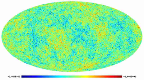
Figure 1: The template of the primordial CMB anisotropies used in the simulations. The map is plotted in units of $\mu K$

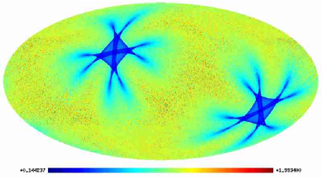
Figure 2: The noise rms variation across the sky, in Galactic coordinates, due to uneven coverage resulting from a sinusoidal-precession scanning strategy with $\theta=90\degr$, $\Delta\theta=7\degr$, opening angle $\phi=85\degr$ and $n_{cycle}=4$. The plot is scaled such that unity corresponds to the average noise rms. Note that the noise rms decreases near the ecliptic poles.

Anisotropic, uncorrelated instrumental noise is simulated for the sinusoidal-precession scanning strategy with $\theta=90\degr$, $\Delta\theta=7\degr$, opening angle $\phi=85\degr$ and $n_{\rm cycle}=4$. The ecliptic latitude $\beta$ depends on the ecliptic longitude $\lambda$ as $\beta=\Delta\theta\sin(n_{\rm cycle}\lambda)$. A map of the corresponding sky coverage for this scanning strategy is shown in Fig. 2. All frequency maps are modelled with the same sky coverage for simplicity.

On calculating the ‘statistical weight’ $w_{\ell m}\equiv[\mn@boldsymbol{{\cal N}}^{-1}]_{\ell m,\ell m}$ for each $(\ell,m)$ mode using (5), we might expect some trends and variations along both $\ell$ and $m$. For this particular scanning strategy, however, with full sky coverage the variations are not very large. In Fig. 3 we plot the relative amplitude of the statistical weights for the 100 GHz channel on large scales ($\ell\leq 200$). It is clear from the plot that the deviations from the average level do not exceed the 10 per cent level.

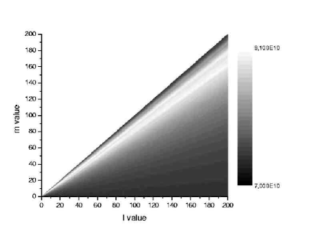
Figure 3: The statistical weight $w_{\ell m}$ of each $(\ell,m)$ mode for the 100 GHz HFI frequency channel assuming the scanning strategy illustrated in Fig. 2. In the case of uniform noise $w_{\ell m}=6.1\times 10^{10}$ (MJy/Sr)^-2 for this channel.

As mentioned above, a cut-sky map can be considered as an extreme case of anisotropic noise. To test the accuracy of the component separation in the presence of a cut, we also prepared a set of channel maps with a symmetric, constant-latitude cut of $\pm 10\degr$ applied along the Galactic plane. In the remainder of the map, we preserved the anisotropic noise pattern resulting from the uneven coverage produced by our assumed scanning strategy, but in the cut region the noise rms was considered as formally infinite. As might be expected, an extreme anisotropy of this sort leads to more profound variations in the statistical weight $w_{\ell m}$ of the modes. In Fig. 4, we plot $w_{\ell m}$ for the 100 GHz channel in this case. It is easy to see from the plot that the deviations from the average level are significant.

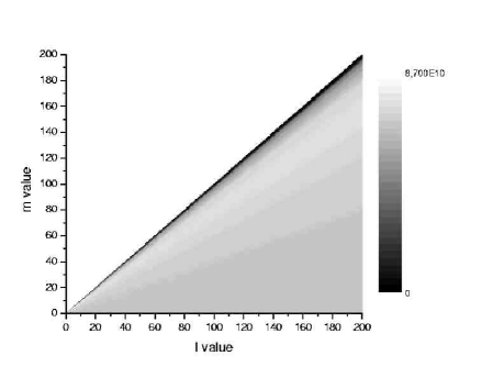
Figure 4: As in Fig. 3, but for a map containing a symmetric, constant-latitude cut of $\pm 10\degr$ along the Galactic plane.

2.2 Results for all-sky data

We first performed a component separation of simulated data with the anisotropic noise distribution shown in Fig. 2, assuming diagonal inverse noise covariance matrices ${\textbf{{N}}}^{-1}_{\ell m}$ with elements given by (11). The reconstructed map obtained for each physical component was of a similar visual quality to those obtained in S02, and so they are not presented here. Instead, we plot only the residuals of the reconstruction of the primordial CMB component in Fig. 5. We see that these residuals are essentially featureless, except for a small band in the Galactic plane. We note, however, that the residuals do contain a faint imprint of the noise rms distribution plotted in Fig. 2.

In Fig. 6 we present the unbiased estimator (see S02) of the CMB power spectrum, obtained from the reconstructed modes for this component, and compare it with the power spectrum of the input primordial CMB realisation used in the simulations. We see from the figure that, even in the presence of realistic anisotropic noise, the reconstructed CMB power spectrum follows the input spectrum out to $\ell\approx 2500$, recovering the correct positions and heights of the first seven acoustic peaks.

In fact, even without making use of our prior knowledge of the noise anisotropy, the effect of the spatially-varying noise rms on the reconstructions is negligible. In order to compare our new approach with that presented in S02, we analysed the same simulated data once more, but assuming that the noise was in fact isotropic. The resulting recovered maps were visually indistingushable from those obtained using the approach outlined above. In Fig 7, we plot the difference in the unbiased estimators of the CMB power spectrum obtained by the two methods. We see that the two approaches yield almost identical results. This is not too surprising, since the variation in the values of the statistical weight per $(\ell,m)$ mode are quite small in the all-sky case, as illustrated in Fig. 3.

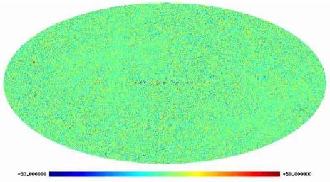
Figure 5: The residuals of the CMB anisotropy reconstruction. The map is plotted in units of $\mu K$

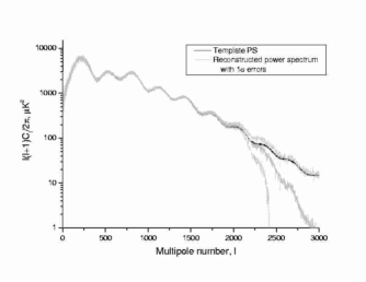
Figure 6: Initial and unbiased reconstructed CMB power spectra for the modelled data with non-uniform pixel noise. The 1$\sigma$ errors on the reconstructed power spectrum are also shown.

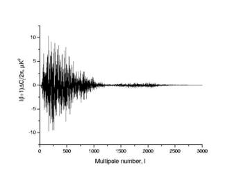
Figure 7: The difference in the unbiased estimators of the CMB power spectrum obtained assuming uniform noise across the sky, and by taking into account noise rms variations.

2.3 Results for cut-sky data

In the process of foreground removal from CMB data (as opposed to component separation), it is common practice to impose some cut along the Galactic plane prior to performing the analysis. In S02, it was shown that such an approach is unnecessary, since accurate results may be obtained by instead performing the component separation on all-sky data, and then imposing a Galactic cut in the reconstructed CMB map, if required, prior to any further analysis. Nevertheless, the question of analysing cut-sky data sets might occur, for example, in the event of instrument failure, and it is thus of interest to investigate how to accommodate this complication.

To test our approach of modelling cut-sky data as an extreme case of anisotropic noise, we performed a component separation using a set of frequency maps with $\pm 10\degr$ symmetrical, constant-latitude cut along the Galactic plane, within which the pixels were set to zero. In Fig. 8 we show the reconstruction of the primordial CMB component, and the corresponding residuals are shown in Fig. 9.

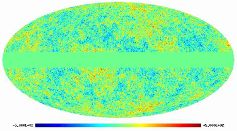
Figure 8: The reconstruction of the CMB anisotropy in the cut-sky case. The map is plotted in units of $\mu K$

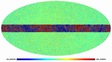
Figure 9: The residuals of the reconstruction in cut-sky case. The map is plotted in units of $\mu K$

The reconstructed physical components were not explicitly restricted to be zero in the cut. Instead, as explained above, the reconstruction was simply not constrained by the data in the cut region. As a result the reconstruction of spherical harmonic modes that lie predominantly in the cut will be prior driven. Since the maximum of the entropic prior occurs for zero signal, such modes will have zero amplitude in the reconstruction. This does not mean, however, that the reconstructed temperature map will be precisely zero in the cut. Modes that are not restricted to the cut region will have amplitudes that are constrained to be non-zero by data on the un-cut part of the sky. Such modes may, in general, contribute to the reconstructed pixel values in the cut region.

We note from Fig. 8 and Fig. 9 that, by using our approach, the quality of the CMB reconstruction outside the cut is unaffected by the presence of the cut. In particular, we see that the reconstruction residuals are featureless over the un-cut part of the sky, and show no identifiable structure even directly adjacent to the cut region. In making this observation, it should also be remembered that no smoothing was applied to the edges of the cut prior to the analysis.

Finally, in Fig. 10, we plot the unbiased estimator (see S02) of the CMB power spectrum, obtained from the reconstructed modes for this component, and compare it with the power spectrum of the input primordial CMB realisation used in the simulations. We see that, even in the presence of the cut, the reconstructed CMB power spectrum follows the input spectrum out to $\ell\approx 2500$.

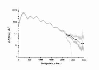
Figure 10: Initial and unbiased reconstructed CMB power spectra for data containing a Galactic cut. The 1$\sigma$ errors on the reconstructed power spectrum are also shown.

3 Spatially-varying foreground spectra

Another major problem for harmonic-space component separation methods, such as MEM and Wiener filtering, is the implicit assumption in (1) that the emission from each physical component can be factorised into a spatial template at some reference frequency $\nu_{0}$ and a frequency dependence, so that

$$I_{\nu}({\hat{\textbf{{x}}}})=\sum_{c=1}^{n_{c}}s_{c}({\hat{\textbf{{x}}}})f_{c}(\nu).$$ (12)

This clearly represents the idealised case in which the spectral parameters of each component do not vary with direction on the sky. In terms of the detailed operation of the harmonic-space MEM algorithm (and Wiener filtering), this assumption is quite central. The MEM approach seeks to find the most probable values for the harmonic coefficients a of the astrophysical components, given the observed data and an entropic regularisation prior on the solution. At each step in the optimisation, the predicted data corresponding to the current best estimate of a is compared (through the Gaussian likelihood function) with the real data. In calculating the predicted data at each frequency, one must determine the contribution of the physical components at this frequency by scaling the solution from the reference frequency $\nu_{0}$ using the conversion matrix $F_{\nu c}$. This matrix determines the frequency behaviour of the components and its coefficients are calculated in accordance to some model of spectral scaling – power law for the synchrotron, modified blackbody emission law for the dust emission, and so on. The scaling is taken to be the same for all $(\ell,m)$ modes, which implies that the parameters defining the spectral scaling do not vary across the sky.

The assumption of spatially-invariant spectral parameters is reasonable for the primordial CMB and the two SZ effects. The thermal SZ effect does depend on the electron temperature of the clusters $T_{e}$, which can reach 10–15 keV; this dependence is rather weak, but can be used to determine $T_{e}$ during component separation, as will be explored in a forthcoming paper. For the Galactic components, however, our assumption is clearly not valid. For example, as discussed in Section 1, the spectral indices of the synchrotron and thermal dust emission are known to vary considerably across the sky. In the case of Planck observations, variation in the synchrotron spectral index will not cause severe problems. Even in the lowest frequency channel at $\nu=30$ GHz, the synchrotron emission is quite weak. A similar conclusion may be drawn for free-free emission. Unfortunately, variations in the spectral parameters of thermal dust emission can give rise to severe difficulties in performing component separation for Planck data.

In the previous simulations presented in S02, the thermal dust emission was assumed to follow a simple single-component grey-body model with spectral emissivity index $\beta=2$ and mean dust temperature $\langle T_{\rm dust}\rangle=18$ K. It is easy to show that variations in these parameters at 20—30 per cent level can lead to differences of the same factor (in specific intensity units) when scaling from the reference frequency $\nu_{0}=300$ GHz to the highest HFI channel at $\nu=857$ GHz. This can cause huge errors in the prediction of dust emission which can reach up to $10^{5}$ MJy/Sr in some regions of the galactic plane. As a result, incorrectly assuming the emissivity and dust temperature to be spatially-invariant can severely reduce the accuracy with which all the physical components are recovered. The dominant cause of these difficulties is in fact the uncertainty in the dust temperature, which is known to vary in the range 5–25 K. It is therefore necessary to take proper account of the variation in the dust temperature to obtain reliable component separation results.

Using the simplest single-component grey-body model as an example, the scaling with frequency of the dust emission can be defined, in terms of specific intensity, by

$$I_{\nu}({\hat{\textbf{{x}}}})=I_{\nu_{0}}({\hat{\textbf{{x}}}})\frac{\nu^{\alpha}B(\nu,T({\hat{\textbf{{x}}}}))}{\nu_{0}^{\alpha}B(\nu_{0},T({\hat{\textbf{{x}}}}))}=I_{\nu_{0}}({\hat{\textbf{{x}}}})F_{\nu c}(T({\hat{\textbf{{x}}}})),$$ (13)

where $I_{\nu}({\hat{\textbf{{x}}}})$ is the dust specific intensity at frequency $\nu$ in the direction ${\hat{\textbf{{x}}}}$, $T({\hat{\textbf{{x}}}})$ is dust colour temperature in this direction, $\beta$ is the emissivity spectral index, which is assumed to be uniform over the sky, and $B(\nu,T)$ is the blackbody function. The quantity $F_{\nu c}(T({\hat{\textbf{{x}}}}))$ is the appropriate element of the conversion matrix for the dust component, which depends on the position on the sky.

Since (13) takes the form of a product of two functions in the spatial domain, we cannot easily pass to the spectral domain, because this product will turn into a convolution over the whole range of the spherical harmonics. In order to work in terms of harmonic coefficients, we instead begin by expanding (13) around the mean dust temperature $T_{0}$ to obtain

$$I_{\nu}({\hat{\textbf{{x}}}})\approx I_{\nu_{0}}({\hat{\textbf{{x}}}})F_{\nu c}(T_{0})+I_{\nu_{0}}({\hat{\textbf{{x}}}})\Delta T({\hat{\textbf{{x}}}})\left.\frac{\partial F_{\nu c}}{\partial T}\right|_{T=T_{0}}+\cdots$$ (14)

where $\Delta T({\hat{\textbf{{x}}}})$ is the deviation from the mean temperature in a given direction. We have not included further terms in the expansion for the sake of brevity, but these may be written down trivially. Given our Taylor series expansion, it is now possible to use our standard formalism to reconstruct several separate (but highly correlated) fields – intensity at the reference frequency $I_{\nu_{0}}$ and intensity-weighted temperature fields $I_{\nu_{0}}\Delta T$, $I_{\nu_{0}}(\Delta T)^{2}$, and so on, to obtain an increasingly accurate approximation to $I_{\nu}({\hat{\textbf{{x}}}})$.

A similar approach may also be used for accommodating spatial variation in any other foreground spectral parameter, such as the dust emissivity or synchrotron spectral index. One may also treat the electron temperature of SZ clusters in the same way. It should be noted, however, that the number of terms used in the Taylor expansion cannot simply increase without limit. Typically, one is constrained such that the total number of fields to be reconstructed does not exceed the number of frequencies at which observations are made.

3.1 Simulated Planck observations

The simulated Planck observations considered here are similar to those described in Section 2.1. We assume six physical components and simulate nine frequency maps, smoothed with appropriate FWHMs and add anisotropic pixel noise. The only difference here is that the thermal dust emission has a spatially-varying temperature distribution.

In simulating the thermal dust emission, it is more accurate to use a two-component best-fit thermal dust model, with the dominant component having a mean temperature of $\langle T_{1}\rangle=16.2$ K and a small contribution of cold dust with $\langle T_{2}\rangle=9.4$ K (Finkbeiner et al. 1999). The two components are fully correlated and their temperature is related by $T_{2}=0.352\,T_{1}^{1.18}$, so we have only one effective temperature parameter. A template for the temperature $T_{1}({\hat{\textbf{{x}}}})$ across the sky was constructed from the colour temperature of Schlegel et al. (1998). The latter was constructed assuming a single-component dust model with the uniform emissivity index of $\beta=2$ and has the mean temperature $\langle T_{\rm dust}\rangle=18$K. This map was simply scaled to $\langle T_{\rm dust}\rangle=16.2K$ to obtain the $T_{1}({\hat{\textbf{{x}}}})$ map for the two-component model used in our simulations (see Fig. 11).

For a multi-component dust model, the dust emission, in specific intensity units, scales with frequency as

$$I_{\nu}({\hat{\textbf{{x}}}}) = I_{\nu_{0}}({\hat{\textbf{{x}}}})\frac{\sum_{k}{f_{k}B(\nu,T_{k}({\hat{\textbf{{x}}}}))q_{k}(\frac{\nu}{\nu_{0}})^{\alpha_{k}}}}{\sum_{k}{f_{k}B(\nu_{0},T_{k}({\hat{\textbf{{x}}}}))q_{k}}}$$ (15)

$$= I_{\nu_{0}}({\hat{\textbf{{x}}}})F_{\nu c}(T({\hat{\textbf{{x}}}})),$$

where $k=1,2,...$ labels the dust component, $f_{k}$ is a normalisation factor for the $k$th component and $\sum_{k}{f_{k}}=1$. The terms $q_{k}(\nu/\nu_{0})^{\alpha_{k}}$ represent the relative emission efficiency for each component (see Finkbeiner et al (1999) for details). For the two-component best-fit model used in our simulations, $f_{1}$=0.0363, $\alpha_{1}$=1.67, $\alpha_{2}$=2.70 and $q_{1}/q_{2}$=13.0 . We can expand the multi-component dust model around the mean temperature an analogous manner to that given in (14) for the single component case.

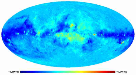
Figure 11: The map of the temperature variations across the sky in K (Schlegel et al. 1998). The original map from Schlegel et al. 1998, with $\langle T_{\rm dust}\rangle=18K$, was scaled to $\langle T_{\rm dust}\rangle=16.2K$ and the mean value has been subtracted.

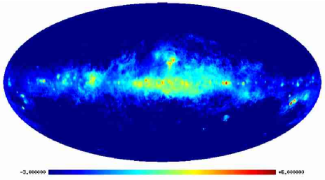
Figure 12: The reconstruction of the colour dust temperature variations $\Delta T_{\rm dust}$. The map is plotted in units of $K$

3.2 Component separation results

Several separation tests were performed to investigate the approach outlined above. In our first test, we recreated the method used in S02, in which the dust temperature was assumed to be spatially-invariant (the zeroth-order approximation), and so only intensity fields $I^{(k)}_{\nu_{0}}$ $(k=1,2,\ldots,6)$ for the six physical components were reconstructed at the reference frequency $\nu_{0}$. In the second test, we attempted to reconstruct 7 components, which included $I^{(k)}_{\nu_{0}}$ for $k=1,2,\ldots,6$, but also the intensity-weighted dust colour temperature field $I_{\nu_{0}}\Delta T$ (the first order of the expansion). Finally, in a third test, 8 components were reconstructed, namely $I^{(k)}_{\nu_{0}}$ for $k=1,2,\ldots,6$, together with $I_{\nu_{0}}\Delta T$ and $I_{\nu_{0}}(\Delta T)^{2}$, thereby accounting for dust temperature variations up to second order.

3.2.1 Quality of the CMB reconstruction

The reconstruction of the primordial CMB component and the corresponding residuals are shown in Fig. 13 for all three separation tests. It is clear from the figure that the separation assuming $T_{\rm dust}$ to be constant over the sky has a very strong residual signal along the plane of Galaxy on the CMB map, where the dust component is strong. Moreover, we see that the reconstruction outside the Galactic plane is also badly contaminated; this is discussed further in Section 4. We thus conclude that the practice adopted in previous component separation analyses of assuming a spatially-invariant dust temperature leads to CMB reconstructions of unacceptably poor quality. Although we do not plot them here, the reconstructions of the other physical components are found to contain similar artefacts both inside and outside the Galactic plane.

 

 

 

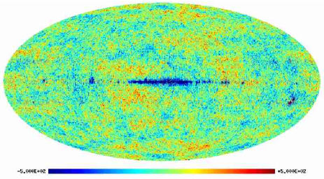
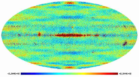
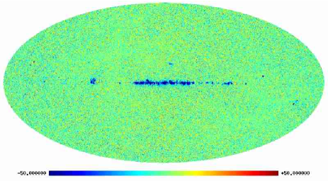
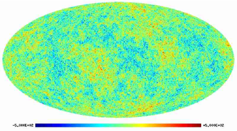
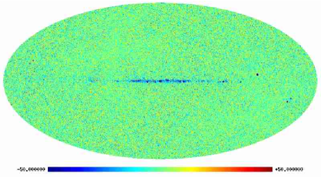
Figure 13: Reconstructions of the primordial CMB component (left-hand column) and the corresponding residuals (right-hand column) for the three separation tests: without any accounting for $T_{\rm dust}$ variations across the sky (top panel); accounting for variations up to first order (middle panel); and accounting for variations up to second order (bottom panel). All maps are plotted in units of $\mu$K.

  

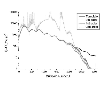
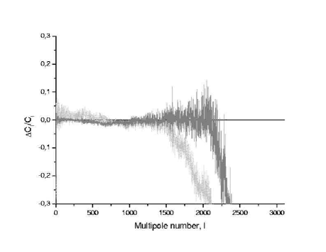
Figure 14: (Left) The input and unbiased reconstructed CMB power spectra for the three separation tests. (Right) The relative difference between the input and reconstructed power spectra $(C^{\rm rec}_{l}-C^{\rm template}_{l})/C^{\rm template}_{l}$ for the second and third cases.

Fortunately, the reconstruction errors are significantly reduced even when the dust temperature variations are accounted for only up to first order in the expansion (14). We see that outside Galactic regions of high dust emission, the CMB residuals in this case are essentially featureless. Nevertheless, the Galactic plane still contains significant dust contamination. The quality of the CMB reconstruction can be improved still further by accounting for $T_{\rm dust}$ variations up to second order. In this case, the remaining contamination of the CMB residuals in the Galactic plane is significantly reduced, to a level comparable to that obtained in S02 in the analysis of simulated data in which $T_{\rm dust}$ was taken not to vary.

A more quantitative comparison of the quality of the CMB reconstructions is given in Fig. 14 (left panel), in which the unbiassed estimates (see S02) of the angular power spectra of the three reconstructions are plotted in relation to the input power spectrum. In each case, the power spectrum has been calculated using the full sky reconstruction. As anticipated from Fig. 13, the recovered power spectrum in the zeroth-order approximation is very poor due to the significant dust contamination. The recovered power spectrum in the first-order approximation is significantly improved. It follows the input spectrum out to $\ell\approx 1700$, recovering the positions and heights of the first 5 acoustic peaks. Beyond this point, the presence of the 6th and 7th acoustic peaks is inferred, but the recovered spectrum begins to underestimate the true power level. In the second-order approximation, the power spectrum recovery is improved still further, and the positions and heights of the first 7 acoustic peaks are accurately recovered before the true power level is again underestimated. The differences between the first and second-order recovered power spectra are further illustrated in the right panel of Fig. 14 in which the ratio $(C^{\rm rec}_{l}-C^{\rm template}_{l})/C^{\rm template}_{l}$ is plotted for these two cases. The improved accuracy and extended range of validity of the second-order approximation is easily seen.

3.2.2 Reconstruction of the dust temperature distribution

For the second and third separation tests, the actual dust colour temperature variations can be calculated as

$$T_{\rm dust}({\hat{\textbf{{x}}}})=\langle T_{\rm dust}\rangle+(I_{\nu_{0}}\Delta T)^{\rm dust}_{{\hat{\textbf{{x}}}}}/I^{\rm dust}_{\nu_{0}}({\hat{\textbf{{x}}}}),$$ (16)

where $I^{\rm dust}_{\nu_{0}}$ is the reconstruction of dust intensity at the reference frequency $\nu_{0}$ assuming the average colour temperature $\langle T_{\rm dust}\rangle$, and $(I_{\nu_{0}}\Delta T)^{\rm dust}$ is the reconstruction of intensity-weighted temperature variation field. The result is shown in Fig. 12. Comparing with Fig. 11, we see that the reconstuction has faithfully recovered the main features of the input map. It is clear, however, that $\Delta T_{\rm dust}$ variations are better restored around the Galactic plane. This is not surprising, since we have actually reconstructed the intensity-weighted $T_{\rm dust}$ field, which can be recoverd more accurately in areas with higher dust intensity, which are obviously located predominantly in the Galactic plane.

4 Discussion and conclusions

In this paper, we have demonstrated an approach that allows one to account for the spatial variations of the noise properties and spectral characteristics of foregrounds in the harmonic-space maximum-entropy component separation technique.

In Section 2.2, we show that the impact of a realistic level of the anisotropic noise on the quality of the foreground separation is quite small, at least for the simple scanning strategy assumed in generating our simulated observations. This can be explained by the fact that the rms noise level differs from the average level only in relatively small areas around ecliptic poles. This leads to variations in the noise level at each harmonic mode that differ from the average value by only a few per cent. We also illustrate in Section 2.2 that the it is possible to perform harmonic-space component separation on cut-sky maps by treating the cut as an extreme example of anisotropic noise. This appraoch has the advantage of not requiring one to smooth the edges of the cut with some apodising function prior to the analysis.

In Section 3, we show that the variation of spectral parameters of foregrounds may be taken into account by a method of succesive approximations based on a series expansion of the corresponding intensity field around the mean value of the parameter. In particular, we investigate the effect of dust colour temperature variations on the quality of the component separation, focussing on the reconstruction of the CMB. We show that realistic dust temperature variations lead to severe contaminaton of the CMB reconstruction if, in the separation process, the dust temperature is assumed not to vary. This contamination is concentrated in the Galactic plane, but significant artefacts exist at high Galactic latitudes. The poor quality of the reconstruction outside the Galactic plane is a result of performing the reconstruction mode-by mode in harmonic space. The inaccurate model of the dust emission leads to errors in the determined amplitudes of a wide range of spherical harmonics in the CMB reconstruction. Many of these modes do not lie predominatly in the Galactic plane region, but contribute to the reconstruction over the whole sky.

If one is content simply with removing foregrounds from the CMB, rather than performing a component separation, then one could apply a Galactic cut prior to the analysis. In Fig. 15, we show the CMB reconstruction and residuals respectively obtained by applying a Galactic cut of $\pm 25\degr$ to each simulated frequency map used in Section 3.1, and assuming a constant dust temperature across the sky.

 

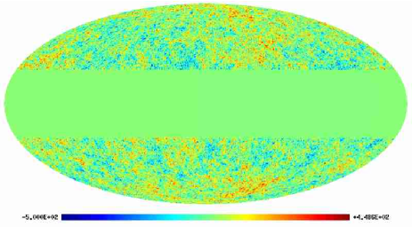
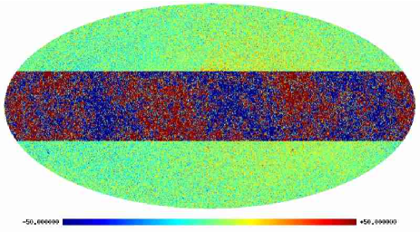
Figure 15: The reconstruction (left) and residuals (right) of the CMB for the case plotted in Fig. 13 (upper row), but with a Galactic cut of $\pm 25\degr$. The maps are plotted in units of $\mu K$.

The noise rms in the cut region was assumed to be formally infinite in the manner discussed in Section 2. We see from the figures that the quality of the reconstruction is significantly improved as compared with the case in which no Galactic cut was applied, which was shown in Fig. 13 (top row). In particular, we note that the residuals now contain no obvious artefacts outside of the cut region. Thus, even assuming an inaccurate dust model, one can still recover a reasonable reconstruction of the CMB outside of the Galactic plane.

It is clearly not possible, however, to perform an acceptable all-sky component separation for the Planck experiment by assuming constant dust spectral parameters, even using all 9 frequency channels. Nevertheless, taking account of dust temperature variations up to first order in the series expansion significantly improves the CMB reconstruction to an acceptable level. This reconstruction quality is still further improved by including second-order terms and is then comparable to that obtained for the ideal case presented in Stolyarov et al. (2002), where the simulated observations assumed no dust temperature variation across the sky. Moreover, an accurate reconstruction of the dust temperature variation is obtained over the whole sky.

Finally we note that the approach for dealing with spatially-varying spectral parameters described in this paper can also be applied to other foregrounds to yield, for example, maps of the synchrotron spectral index. The method can also be used to reconstruct the electron temperature in clusters from their thermal SZ effect, as will be discussed in a forthcoming paper.

5 Acknowledgements

Some of the results in this paper have been derived using HEALPix (Górski, Hivon and Wandelt 1999) package. The authors thank Mark Ashdown for many useful conversations regarding component separation and Daniel Mortlock for supplying anisotropic noise models. Numerical calculations were performed on the National Cosmology Altix 3700 Supercomputer funded by HEFCE and PPARC and in cooperation with Silicon Graphics. RBB thanks the Ministerio de Ciencia y Tecnología and the Universidad de Cantabria for a Ramón y Cajal contract.

Appendix A The noise covariance matrix in the spherical harmonic domain

We consider a single frequency map for which $n_{p}$ is the instrumental noise in the $p$th pixel. We denote the spherical harmonic coefficients of the noise by $\epsilon_{\ell m}$.

The elements of the noise covariance matrix in the harmonic domain are given by

$${\cal N}_{\ell m,\ell^{\prime}m^{\prime}} = \langle\epsilon_{\ell m}\epsilon^{\ast}_{\ell^{\prime}m^{\prime}}\rangle$$ (17)

$$= \langle\Omega_{\rm pix}\sum_{p}\bigl{(}Y_{\ell m}(p)n_{p}\bigr{)}~{}\Omega_{\rm pix}\sum_{p^{\prime}}\bigl{(}Y^{\ast}_{\ell^{\prime}m^{\prime}}(p^{\prime})n_{p^{\prime}}\bigr{)}\rangle$$

$$= \Omega^{2}_{\rm pix}\sum_{p}\sum_{p^{\prime}}Y_{\ell m}(p)Y^{\ast}_{\ell^{\prime}m^{\prime}}(p^{\prime})\langle n_{p}n_{p^{\prime}}\rangle$$

$$= \Omega^{2}_{\rm pix}\sum_{p}Y_{\ell m}(p)Y^{\ast}_{\ell^{\prime}m^{\prime}}(p)\sigma^{2}_{p}$$

where $Y_{\ell m}(p)$ denotes the value of the corresponding spherical harmonic at the $p$th pixel centre, $\Omega_{\rm pix}=4\pi/N_{\rm pix}$ and, in the last line, we have assumed that the noise is uncorrelated between pixels, so that $\langle n_{p}n_{p^{\prime}}\rangle=\sigma^{2}_{p}\delta_{pp^{\prime}}$. We note that in the special case in which the noise is statistically isotropic, $\sigma^{2}_{p}=\sigma^{2}$ for all pixels, and we obtain

$${\cal N}_{\ell m,\ell^{\prime}m^{\prime}} = \Omega_{\rm pix}\sigma^{2}\Bigl{[}\Omega_{\rm pix}\sum_{p}Y_{\ell m}(p)Y^{\ast}_{\ell^{\prime}m^{\prime}}(p)\Bigr{]}$$ (18)

$$= \Omega_{\rm pix}\sigma^{2}\delta_{\ell\ell^{\prime}}\delta_{mm^{\prime}}.$$

It is convenient to define the double indices $i\equiv\ell m$ and $j\equiv\ell^{\prime}m^{\prime}$, and regard (17) as the elements of the noise covariance matrix $\mn@boldsymbol{\cal N}$. One may then write

$$\mn@boldsymbol{\cal N}=\Omega_{\rm pix}^{2}{\textbf{{Y}}}^{\dagger}{\textbf{{N}}}{\textbf{{Y}}},$$ (19)

where N is the noise covariance matrix in the pixel domain, with elements $N_{pp^{\prime}}=\langle n_{p}n_{p^{\prime}}\rangle$, and we have defined the transformation matrix Y with elements $Y_{pi}=Y_{i}(p)$.

Using the fact that transformation matrix has the useful property

$${\textbf{{Y}}}^{\dagger}{\textbf{{Y}}}=\frac{1}{\Omega_{\rm pix}}\textbf{{I}}={\textbf{{Y}}}{\textbf{{Y}}}^{\dagger},$$ (20)

it is straightforward to show that $\mn@boldsymbol{{\cal N}}\mn@boldsymbol{{\cal N}}^{-1}={\textbf{{I}}}=\mn@boldsymbol{{\cal N}}^{-1}\mn@boldsymbol{{\cal N}}$, where the inverse noise covariance matrix in the spherical harmonic domain is given by

$$\mn@boldsymbol{{\cal N}}^{-1}={\textbf{{Y}}}^{\dagger}{\textbf{{N}}}^{-1}{\textbf{{Y}}}.$$ (21)

In the special case that the instrumental noise is uncorrelated between pixels, ${\textbf{{N}}}^{-1}$ is diagonal and we obtain

$$\left[\mn@boldsymbol{{\cal N}}^{-1}\right]_{\ell m,\ell^{\prime}m^{\prime}}=\sum_{p}Y_{\ell m}(p)Y^{*}_{\ell^{\prime}m^{\prime}}(p)\frac{1}{\sigma_{p}^{2}}.$$ (22)

References

- (1) Baccigalupi, C., Bedini, L., Burigana, C., De Zotti, G., Farusi, A., Maino, D., Maris, M., Perrotta, F., Salerno, E., Toffolatti, L., Tonazzini, A., 2000, MNRAS, 318, 769
- (2) Barreiro R.B., Hobson M.P., Banday A.J., Lasenby A.N., Stolyarov V., Vielva P., Górski K.M., 2004, MNRAS, in press (astro-ph/0302091)
- (3) Finkbeiner D.P., Davis M., Schlegel D.J., 1999, ApJ, 524, 867
- (4) Górski K.M., Hivon E., Wandelt B.D., 1999, in Proceedings of the MPA/ESO Cosmology Conference ”Evolution of Large-Scale Structure”, eds. Banday A.J., Sheth R.S. and Da Costa L., PrintPartners Ipskamp, NL, p.37
- (5) Giardino, G., Banday, A.J., Gorski, K.M., Bennett, K., Jonas, J.L., Tauber, J., 2002, A&A, 387, 82
- (6) Hobson M.P., Jones A.W., Lasenby A.N., Bouchet F.R., 1998, MNRAS, 300, 1
- (7) Hobson M.P., Barreiro R.B., Toffolatti L, Lasenby A.N., Sanz J., Jones A.W., Bouchet F.R., 1999, MNRAS, 306, 232
- (8) Jones, A. W., Hobson, M. P., Mukherjee, P., Lasenby, A. N., 2000, ApL&C, 37, 369
- (9) Maino, D., Farusi, A., Baccigalupi, C., Perrotta, F., Banday, A. J., Bedini, L., Burigana, C., De Zotti, G., Górski, K. M., Salerno, E., 2002, MNRAS, 334, 53
- (10) Stolyarov V., Hobson M.P., Ashdown M.A.J., Lasenby A.N., 2002, MNRAS, 336, 97
- (11) Schlegel D.J., Finkbeiner D.P., Davis M., 1998, ApJ, 500, 525
- (12) Vielva P., Barreiro R.B., Hobson M.P., Martínez-González E., Lasenby A.N., Sanz J.L., Toffolatti L., 2001, MNRAS, 328, 1
- (13) Vielva P., Martínez-González E., Gallegos J.E., Toffolatti L., Sanz J.L., 2003, MNRAS, 344, 89