Cross Terms and Weak Frequency Dependent Signals in the CMB Sky

Abstract

In this paper, we study the amplification of weak frequency dependent signals in the CMB sky due to their cross correlation to intrinsic anisotropies. In particular, we center our attention on mechanisms generating some weak signal, of peculiar spectral behaviour, such as resonant scattering in ionic, atomic or molecular lines, thermal SZ effect or extragalactic foreground emissions, whose typical amplitude (denoted by $\epsilon$) is sufficiently smaller than the intrinsic CMB fluctuations. We find that all these effects involve either the autocorrelation of anisotropies generated during recombination ($z_{rec}$) or the cross-correlation of those anisotropies with fluctuations arising at redshift $z_{i}$. The former case accounts for the slight blurring of original anisotropies generated in the last scattering surface, and shows up in the small angular scale (high multipole) range. The latter term describes, instead, the generation of new anisotropies, and is non-zero only if fluctuations generated at redshifts $z_{rec},\;z_{i}$ are correlated. The degree of this correlation can be computed under the assumption that density fluctuations were generated as standard inflationary models dictate and that they evolved in time according to linear theory. In case that the weak signal is frequency dependent, (i.e., the spectral dependence of the secondary anisotropies is distinct from that of the CMB), we show that, by substracting power spectra at different frequencies, it is possible to avoid the limit associated to Cosmic Variance and unveil weaker terms linear in $\epsilon$. We find that the correlation term shows a different spectral dependence than the squared ($\propto\epsilon^{2}$) term considered usually, making its extraction particularly straightforward for the thermal SZ effect. Furthermore, we find that in most cases the correlation terms are particularly relevant at low multipoles due to the ISW effect and must be taken into account when characterising the power spectrum associated to weak signals in the large angular scales.

1 Introduction

Standard theories state that the field of density perturbations arising after the inflationary epoch, ($\delta(\mbox{\bf{x}})\equiv(\rho(\mbox{\bf{x}})-\bar{\rho})/\bar{\rho}$, with $\bar{\rho}$ the average density), should be gaussian, homogeneous and isotropic, (Guth, 1981; Starobinskii, 1981; Mukhanov & Chibisov, 1982; Linde, 1983). The Fourier modes of this field ($\delta_{\mbox{\bf{k}}}$) are predicted to have independent real and imaginary components, which should be gaussian distributed from a scale-invariant power spectrum, (Harrison–Zel’dovich, (HS), (Zeldovich, 1972)), i.e., $\langle\delta_{\mbox{\bf{k}}}\delta_{\mbox{\bf{q}}}^{*}\rangle=(2\pi)^{3}P(k)\delta_{D}(\mbox{\bf{k}}+\mbox{\bf{q}})$, with $P(k)\propto k$. This power spectrum determines the properties of the spatial correlation of the perturbation field, since it is the mere Fourier transform of the correlation function. These perturbations are small compared to the homogeneous background, ($|\delta|\ll 1$), but grow up due to gravitational instabilities. This growth is independent for each mode, i.e., mode coupling can be neglected, as long as the perturbations remain small and linear theory can be applied.

From the observational point of view, the first test ground for this perturbation field is the study of the temperature anisotropies of the Cosmic Microwave Background (CMB). Most of these temperature fluctuations were generated by energy density inhomogeneities in the universe during the epoch at which most electrons and protons recombined to form hydrogen and radiation decoupled from matter, (last scattering surface, LSS). At this stage, the density inhomogeneities were still under linear regime, provided that the amplitude of typical measured CMB temperature fluctuations are one part in one hundred thousand, (e.g. Smoot et al. (1991); Bennett et al. (2003a)). In their transit from the LSS towards us, the CMB photons witnessed the matter collapse and formation of non linear structures such as galaxies, clusters of galaxies, filaments and superclusters of galaxies that today conform the visible universe. The crossing through these scenarios imprinted on the CMB photons new temperature anisotropies, which are usually labelled as secondary. The amplitude of these secondary anisotropies is, in many cases, few orders of magnitude below the level of the primary ones generated in the LSS. However, the different spectral behaviour of some of them might help in the distinction from the primary. In this context, the presence of foregrounds, galactic or extragalactic, with their own spectral dependence, will make the picture furtherly more complicated.

Consequently, a major issue in current CMB science is the accurate component separation in future microwave maps. From the observation point of view, a set of space and groundbased experiments with unprecendented sensitivity and angular resolution, counting with several broad band detectors spread in appropiate frequency ranges, are being proposed or already under development, (e.g., Planck, ACT(Kosowsky, 2003), South Pole Telescope,QUIET or CMBPOL). In the theoretical side, new analysis techniques of temperature maps, based both in real and Fourier space, and dealing with second (correlation function, power spectrum) and higher order momenta of quantities derived from the temperature field are being developed and tested on simulated data. Nevertheless, the two main limiting factors in this task will be i) the instrumental noise and instrument systematics and ii) the cosmic variance, associated to the fact that our characterization of the universe is statistical, but based on a single realization of it.

In this work, we study the spatial correlation of density fluctuations in the universe, and how this reflects in the CMB angular power spectrum. These aspects must be taken into account if an accurate characterization of the CMB power spectrum is to be achieved, particularly at the large angular (low multipole) scales. This study also allows us to propose a method that uses observations in different frequencies and combines power spectra in such a way that avoids the limitation imposed by cosmic variance, and unveils weak signals whose amplitude $\sigma_{w}$ is in the range $\sigma_{N}>\sigma_{w}>\sigma_{N}\left(\sigma_{N}/\sigma_{t}\right)$, where $\sigma_{N}$ is the experimental noise amplitude and $\sigma_{t}$ is the typical amplitude of a dominant signal $t$ which is assumed to be totally correlated to the weak signal $w$. This approach was already utilized in Basu, Hernández-Monteagudo & Sunyaev (2004) when charactering the effect of metal atoms and ions on the CMB during the secondary ionization.

In Section 2 we outline our method, which we apply in Section 3 on particular physical mechanisms generating secondary fluctuations in two different cosmological scenarios. In Section 4 we comment our results and conclude.

2 Comparing Second Order Momenta

2.1 The Flat Case

Our starting point will be the superposition of two signals, $g_{1}(\nu)\;t_{1}$ and $g_{2}(\nu)\;t_{2}$, whose amplitudes will show, a priori, a different frequency ($\nu$) dependence. In real space they give rise to

$$T(\mbox{\bf{x}},\nu)=g_{1}(\nu)t_{1}(\mbox{\bf{x}})+g_{2}(\nu)\epsilon t_{2}(\mbox{\bf{x}})+N_{\nu}(\mbox{\bf{x}}),$$ (1)

and analogously, in Fourier space, to

$$T_{\mbox{\bf{k}}}(\nu)=g_{1}(\nu)t_{1,\mbox{\bf{k}}}+g_{2}(\nu)\epsilon t_{2,\mbox{\bf{k}}}+N_{\nu,\mbox{\bf{k}}},$$ (2)

where k is the Fourier mode under consideration. If we assume that $g_{1}(\nu_{1})t_{1}$ and $g_{2}(\nu_{2})t_{2}$ are of similar amplitude, then the parameter $\epsilon$ gives the relative amplitude of both signals , and for the cases considered below, we shall take $\epsilon\ll 1$. $N_{\nu}$ is the noise component present in the map. Now let us assume that the experiment is able to observe at two different frequencies $\nu_{1},\nu_{2}$. Defining $f\equiv g_{1}(\nu_{1})/g_{1}(\nu_{2})$, we find that:

$$\delta\left(T^{2}(\mbox{\bf{x}},\mbox{\bf{y}})\right)\equiv\;T(\mbox{\bf{x}},\nu_{1})T(\mbox{\bf{y}},\nu_{1})-f^{2}T(\mbox{\bf{x}},\nu_{2})T(\mbox{\bf{y}},\nu_{2})\;=$$

$$\phantom{xx}\epsilon\;\;g_{1}(\nu_{1})g_{2}(\nu_{2})\left[1-\frac{g_{1}(\nu_{1})}{g_{1}(\nu_{2})}\frac{g_{2}(\nu_{2})}{g_{2}(\nu_{1})}\right]\left[t_{1}(\mbox{\bf{x}})t_{2}(\mbox{\bf{y}})+t_{1}(\mbox{\bf{y}})t_{2}(\mbox{\bf{x}})\right]$$

$$\phantom{xx}+\epsilon^{2}\;\;g_{2}^{2}(\nu_{1})\left[1-\left(\frac{g_{1}(\nu_{1})}{g_{1}(\nu_{2})}\frac{g_{2}(\nu_{2})}{g_{2}(\nu_{1})}\right)^{2}\right]t_{2}(\mbox{\bf{x}})t_{2}(\mbox{\bf{y}})$$

$$\phantom{xx}+N_{\nu_{1}}(\mbox{\bf{x}})N_{\nu_{1}}(\mbox{\bf{y}})-f^{2}\;N_{\nu_{2}}(\mbox{\bf{x}})N_{\nu_{2}}(\mbox{\bf{y}})$$

$$\phantom{xx}+{\cal O}\left[N_{\nu_{1}},N_{\nu_{2}}\right],$$ (3)

or, in Fourier space,

$$\delta\left(T_{\mbox{\bf{k}},\mbox{\bf{q}}}^{2}\right)\equiv T_{\mbox{\bf{k}}}(\nu_{1})T_{\mbox{\bf{q}}}(\nu_{1})-f^{2}T_{\mbox{\bf{k}}}(\nu_{2})T_{\mbox{\bf{q}}}(\nu_{2})=$$

$$\phantom{xx}\epsilon\;g_{1}(\nu_{1})g_{2}(\nu_{1})\left[1-\frac{g_{1}(\nu_{1})}{g_{2}(\nu_{2})}\frac{g_{2}(\nu_{2}}{g_{2}(\nu_{1})}\right]\left[t_{1,\mbox{\bf{k}}}t_{2,\mbox{\bf{q}}}+t_{2,\mbox{\bf{k}}}t_{1,\mbox{\bf{q}}}\right]$$

$$\phantom{xx}+\epsilon^{2}\;\;g_{2}^{2}(\nu_{1})\left[1-\left(\frac{g_{1}(\nu_{1})}{g_{2}(\nu_{2})}\frac{g_{2}(\nu_{2}}{g_{2}(\nu_{1})}\right)^{2}\right]\;\;t_{2,\mbox{\bf{k}}}t_{2,\mbox{\bf{q}}}$$

$$\phantom{xx}+N_{\nu_{1},\mbox{\bf{k}}}N_{\nu_{1},\mbox{\bf{q}}}-f^{2}\;N_{\nu_{2},\mbox{\bf{k}}}N_{\nu_{2},\mbox{\bf{q}}}$$

$$\phantom{xx}+{\cal O}\left[N_{\nu_{1}},N_{\nu_{2}}\right].$$ (4)

${\cal O}\left[N_{\nu_{1}},N_{\nu_{2}}\right]$ in both equations refers to cross terms of the noise field with all the other components at a given frequency. These two equations should be compared to the squared difference map, ($\left(\delta T\left(\mbox{\bf{x}},\mbox{\bf{y}}\right)\right)^{2}$, $\left(\delta T_{\mbox{\bf{k}},\mbox{\bf{q}}}\right)^{2}$), given by:

$$\left(\delta T\left(\mbox{\bf{x}},\mbox{\bf{y}}\right)\right)^{2}\equiv$$

$$\phantom{xx}\left(T(\mbox{\bf{x}},\nu_{1})-fT(\mbox{\bf{y}},\nu_{2})\right)\left(T(\mbox{\bf{x}},\nu_{1})-fT(\mbox{\bf{y}},\nu_{2})\right)=$$

$$\phantom{xx}\epsilon^{2}\;\large(\;\left[g_{2}(\nu_{1})\;t_{2}(\mbox{\bf{x}})\right]^{2}\;+\left[f\;g_{2}(\nu_{2})\;t_{2}(\mbox{\bf{y}})\right]^{2}-$$

$$\phantom{xxxxxxxxxxxx}2\;f\;g_{2}(\nu_{1})g_{2}(\nu_{2})t_{2}(\mbox{\bf{x}})t_{2}(\mbox{\bf{y}})\;\large)\;+$$

$$\phantom{xx}N_{\nu_{1}}^{2}(\mbox{\bf{x}})+N_{\nu_{1}}^{2}(\mbox{\bf{y}})+{\cal O}\left[N_{\nu_{1}},N_{\nu_{2}}\right],$$ (5)

in real space, and

$$\left(\delta T_{\mbox{\bf{k}},\mbox{\bf{q}}}\right)^{2}\equiv$$

$$\phantom{xx}\left(T_{\mbox{\bf{k}}}(\nu_{1})-fT_{\mbox{\bf{q}}}(\nu_{2})\right)\left(T_{\mbox{\bf{k}}}(\nu_{1})-fT_{\mbox{\bf{q}}}(\nu_{2})\right)=$$

$$\phantom{xx}\epsilon^{2}\;\;\large(\left[t_{2,\mbox{\bf{x}}}g_{2}(\nu_{1})\right]^{2}+\left[ft_{2,\mbox{\bf{y}}}g_{2}(\nu_{2})\right]^{2}-$$

$$\phantom{xxxxxxxxxxxx}2\;f\;g_{2}(\nu_{1})g_{2}(\nu_{2})t_{2,\mbox{\bf{x}}}t_{2,\mbox{\bf{y}}}\;\large)\;+$$

$$\phantom{xx}N_{\nu_{1},\mbox{\bf{k}}}^{2}+N_{\nu_{1},\mbox{\bf{q}}}^{2}+{\cal O}\left[N_{\nu_{1}},N_{\nu_{2}}\right]$$ (6)

in Fourier space.

It is clear that for $\epsilon\ll 1$, $\delta\left(T^{2}(\mbox{\bf{x}},\mbox{\bf{y}})\right)$ or $\delta\left(T_{\mbox{\bf{k}},\mbox{\bf{q}}}^{2}\right)$ are much more sensitive to the weak signal $\epsilon t_{2}$ than $\left(\delta T\left(\mbox{\bf{x}},\mbox{\bf{y}}\right)\right)^{2}$ or $\left(\delta T_{\mbox{\bf{k}},\mbox{\bf{q}}}\right)^{2}$. The obvious difference is the term linear in $\epsilon$ present in eqs.(3,4). However, in the context of Cosmology and CMB, one counts with only one single realization of the Universe, and the quantities defined above as $\delta\left(T^{2}(\mbox{\bf{x}},\mbox{\bf{y}})\right)$ or $\delta\left(T_{\mbox{\bf{k}},\mbox{\bf{q}}}^{2}\right)$ must be averaged either in real or Fourier space, in order to acquire some statistical meaning, (i.e., if averaged under certain conditions, they yield estimates of the correlation function and the power spectrum, respectively). After this average, the term linear in $\epsilon$ becomes proportional to $\langle t_{1}\;t_{2}\rangle$, and will not average out if and only if both signals $t_{1}$, $t_{2}$ are correlated, at least to some extent. Therefore, in order for this cross term to be of any utility, both the dominant and the weak signals must be correlated. We shall show below that this is indeed the case for signals coupled to linear fluctuations of the density field generated after inflation. Another point to remark is that, because of substracting quantities computed from the same maps, one exactly cancels the dominant signal, leaving no room for the uncertainty due to the cosmic variance associated to it. This allows the weak signal be under the limit imposed by the cosmic variance of the dominant one.

As mentioned in the Introduction, in linear theory all Fourier modes $\delta_{\mbox{\bf{k}}}$ of the density fluctuations evolve independently according to a growth factor $D(\eta)$ ($\eta$ is conformal time) which is dependent on the cosmological parameters of our universe. These modes are all independent, and for reasons associated to the homogeneity and isotropy, must depend exclusively on the modulus of the k vectors, $k$. This allows writing the power spectrum as $\langle\delta_{\mbox{\bf{k}}}\delta_{\mbox{\bf{q}}}\rangle=(2\pi)^{3}P(k)\delta_{D}(\mbox{\bf{k}}+\mbox{\bf{q}})$. In an analogous way, the averages of the product of all pair of quantities depending linearly on $\delta_{\mbox{\bf{k}}}$ will be proportional to the power spectrum. This applies practically to all perturbations of physical quantities, such as peculiar velocities or gravitational potentials, that are responsible for the generation of temperature anisotropies in the CMB.

The average in our maps will be performed in the real space in such a way that the distance between x and y is kept constant. In Fourier space, we shall take q equal to $-\mbox{\bf{k}}$, fix the modulus (k) and average over the mode phases. The former will yield the correlation function, the latter the power spectrum. This average also removes all cross terms in noise. Furthermore, if we assume that the statistical properties of noise have been characterized, then it is possible to substract the expectations for the terms quadratic in noise in eqs.(3,4), and the residuals of this substraction can be treated as random variables. These random residuals should be regarded as the effective noise in our correlation function or power spectrum estimates, and will be denoted by $\Delta N_{\nu,\mbox{\bf{x}}-\mbox{\bf{y}}}$ and $\Delta N_{\nu,k}$:

$$\Delta N_{\nu,\mbox{\bf{x}}-\mbox{\bf{y}}} \equiv {\cal E}\bigl{(}\langle N_{\nu}(\mbox{\bf{x}})N_{\nu}(\mbox{\bf{y}})\rangle\bigr{)}-\langle N_{\nu}(\mbox{\bf{x}})N_{\nu}(\mbox{\bf{y}})\rangle_{EXP}$$ (7)

$$\Delta N_{\nu,k} \equiv {\cal E}\bigl{(}\langle N_{\nu,\mbox{\bf{k}}}N_{\nu,-\mbox{\bf{k}}}\rangle\bigr{)}-\langle N_{\nu,\mbox{\bf{k}}}N_{\nu,-\mbox{\bf{k}}}\rangle_{EXP},$$ (8)

where ${\cal E}$ and the label EXP denote estimated on the map and expected values, respectively. We are assuming that noise in different frequencies is uncorrelated. For the case of gaussian white noise, it is easy to prove that $\langle\Delta N_{\nu,\mbox{\bf{x}}-\mbox{\bf{y}}}\rangle=\langle\Delta N_{\nu,k}\rangle=0$, (assuming a correct characterization of noise), and that

$$\langle\Delta N_{\nu,\mbox{\bf{x}}-\mbox{\bf{y}}}^{2}\rangle = \frac{2}{n}\langle N_{\nu}(\mbox{\bf{x}})N_{\nu}(\mbox{\bf{y}})\rangle_{EXP}^{2}$$ (9)

$$\langle\Delta N_{\nu,k}^{2}\rangle = \frac{2}{n}\langle N_{\nu}(\mbox{\bf{k}})N_{\nu}(-\mbox{\bf{k}})\rangle_{EXP}^{2}.$$ (10)

$n$ is the number of points, either in real of Fourier space, used when estimating the averages. Having this in mind, we can perform the averages and rewrite eqs.(3,4) like

$${\cal E}\bigl{(}\langle\delta\left(T^{2}(\mbox{\bf{x}},\mbox{\bf{y}})\right)\rangle\bigr{)}=$$

$$\epsilon\;\;g_{1}(\nu_{1})g_{2}(\nu_{2})\left[1-\frac{g_{1}(\nu_{1})}{g_{1}(\nu_{2})}\frac{g_{2}(\nu_{2})}{g_{2}(\nu_{1})}\right]2\;\langle t_{1}(\mbox{\bf{x}})t_{2}(\mbox{\bf{y}})\rangle$$

$$\phantom{xxxxxxxxxx}\pm\Delta_{N}\;+\;{\cal O}\left[\epsilon^{2}\right]$$ (11)

and

$${\cal E}\bigl{(}\langle\delta\left(T_{\mbox{\bf{k}},-\mbox{\bf{k}}}^{2}\right)\rangle\bigr{)}\;=$$

$$\epsilon\;g_{1}(\nu_{1})g_{2}(\nu_{1})\left[1-\frac{g_{1}(\nu_{1})}{g_{1}(\nu_{2})}\frac{g_{2}(\nu_{2})}{g_{2}(\nu_{1})}\right]\langle t_{1,\mbox{\bf{k}}}t_{2,-\mbox{\bf{k}}}+t_{2,\mbox{\bf{k}}}t_{1,-\mbox{\bf{k}}}\rangle\;$$

$$\phantom{xxxxxxxxxx}\pm\Delta_{N}\;+\;{\cal O}\left[\epsilon^{2}\right].$$ (12)

$\Delta_{N}$ is the residual noise contribution, $\Delta_{N}^{2}=\langle\Delta N_{\nu_{1}}^{2}\rangle+f^{2}\langle\Delta N_{\nu_{2}}^{2}\rangle$ in both real and Fourier space, (eqs.(9–10)). From this equation, one can see that the approach proposed here will be sensitive to $\epsilon\;t_{2}$ if:

$$\omega\;\epsilon>\frac{\sigma_{N}^{2}}{\sigma_{t}^{2}}\times\frac{\sqrt{\frac{2}{n}\left(1+f^{2}\right)}}{2\cdot\left(1-\frac{g_{1}(\nu_{1})g_{2}(\nu_{2})}{g_{1}(\nu_{2})g_{2}(\nu_{1})}\right)},$$ (13)

with $\sigma_{N}^{2}\equiv\langle N_{\nu}^{2}(\mbox{\bf{x}})\rangle$ taken equal for the two frequencies and $\sigma_{t}^{2}\equiv g_{1}^{2}(\nu_{1})\langle t_{1}^{2}\rangle\sim g_{2}^{2}(\nu_{2})\langle t_{2}^{2}\rangle$. The factor $\omega$ accounts for the cross correlation between $t_{1}$ and $t_{2}$, i.e., $\omega\equiv\langle t_{1}\cdot t_{2}\rangle/\sigma_{t}^{2}$, (note that in the absence of correlation, $\omega=0$ since we are taking $\langle t_{1}\rangle=0$ by construction). Let us remark that the limit on $\omega\epsilon$ is roughly an order in $\sigma_{N}/\sigma_{t}$ beyond the limit imposed on $\epsilon$ by eqs. (5,6). Note that in the case of similar frequency dependence for the two signals, ($g_{1}(\nu)\simeq g_{2}(\nu)$), this method cannot work. For similar reasons, if $g_{1}(\nu)\neq g_{2}(\nu)$, then it should be possible, a priori, to perform as many consistency checks in different frequencies as the instrument permits, since the correlation term should vary its amplitude as dictated by the frequency dependent term

$$\Gamma(\nu_{1},\nu_{2})\equiv g_{1}(\nu_{1})g_{2}(\nu_{1})\left[1-\frac{g_{1}(\nu_{1})}{g_{1}(\nu_{2})}\frac{g_{2}(\nu_{2})}{g_{2}(\nu_{1})}\right].$$ (14)

From this formalism, it follows that the importance of this approach relies i) on the amplitude of the cross-correlation between the signals under consideration and ii) on their spectral dependence. Let us remark as well that this method is sensitive to the relative sign of the two signals. In the context of the CMB, this correlation will preferrably show up in the low multipole range: at these large angular scales the instrumental sensitivity performs best, but the removal of galactic foregrounds becomes particularly difficult. In the next section, we shall address several scenarios where this correlation may be relevant, and discuss under which conditions the method proposed here becomes useful.

The approach outlined here is complementary, but different, to that used in, e.g., Banday et al. (1996), Kneissl et al. (1997), Rubiño-Martín, Atrio-Barandela, & Hernández-Monteagudo (2000), and more recently, Boughn & Crittenden (2003), Fosalba, Gaztañaga & Castander (2003) and Hernández-Monteagudo & Rubiño-Martín (2004). In all those cases, the weak signal ($\epsilon t_{2}$) was not considered to be correlated to the dominant signal, but it was cross-correlated to an external template: this cross-correlation retained only the term linear in $\epsilon$, and hence no substraction was required.

Hereafter, the term proportional to $\epsilon$ will be referred to as the linear or cross term, whereas the term proportional to $\epsilon^{2}$ will be denoted as the squared term.

2.2 Correlations Projected on the Sphere

In this subsection we briefly outline the formalism that describes the analysis of temperature fluctuations in the CMB. It is customary to work in the spherical Fourier space, in which the coefficients $a_{l,m}$’s define a temperature field in the celestial sphere through the following decomposition on spherical harmonics:

$$\frac{\delta T}{T_{0}}(\theta,\phi)=\sum_{l,m}a_{l,m}\;Y_{l,m}(\theta,\phi).$$ (15)

The power spectrum for an arbitrary temperature field is obtained after averaging the Fourier coefficients,

$$C_{l}\equiv\langle a_{l,m}a_{l,m}^{*}\rangle.$$ (16)

Having this in mind, the analysis of weak signals outlined in the previous section translates into the spherical case as

$$\delta C_{l}=2\epsilon\Gamma(\nu_{1},\nu_{2})\langle a_{l,m}(a_{l,m}^{weak})^{*}\rangle+{\cal O}[\epsilon^{2}].$$ (17)

However, when computing this correlations, it will be convenient to express the $a_{l,m}$’s as integrals in the flat Fourier space. Indeed, the temperature field can be decomposed in Fourier modes as (e.g.,Hu & Sugiyama (1995)):

$$\Delta\left(\mbox{\bf{k}},{\bf n},\eta_{0}\right)=\int d\mbox{\bf{x}}\frac{\delta T}{T_{0}}(\mbox{\bf{x}},{\bf n},\eta_{0})\;e^{-i\mbox{\bf{k}}\mbox{\bf{x}}}=$$

$$\phantom{xxxxxxxxxx}\sum_{l}(-i)^{l}\left(2l+1\right)P_{l}(\mu)\Delta_{l}(\mbox{\bf{k}},\eta_{0}),$$ (18)

with $\mu=\hat{{\bf k}}\cdot\hat{{\bf n}}$, and $\hat{{\bf n}}$ is the pointing vector on the sky given by $(\theta,\;\phi)$. $\eta_{0}$ denotes the conformal time evaluated at the present epoch. The last step shows the expansion on a Legendre polynomial basis, and assumes implicitely that perturbations are axially symmetric about k, (e.g., Ma & Bertschinger (1995)). From this, it is straightforward to show that, for $\mbox{\bf{x}}=0$, the $a_{l,m}$ multipoles can be written as:

$$a_{l,m}=\left(-i\right)^{l}\;4\pi\;\int d\mbox{\bf{k}}Y_{l,m}^{*}(\hat{k})\;\Delta_{l}(\mbox{\bf{k}},\eta).$$ (19)

In linear theory, $\Delta_{l}(\mbox{\bf{k}},\eta)=\Delta_{l}(k,\eta)\psi_{i}\left(\mbox{\bf{k}}\right)$, with $\psi_{i}\left(\mbox{\bf{k}}\right)$ the initial scalar perturbations and $\langle\psi_{i}\left(\mbox{\bf{k}}\right)\psi_{i}\left(\mbox{\bf{q}}\right)\rangle=P_{\psi}\left(k\right)\left(2\pi\right)^{3}\delta_{D}\left(\mbox{\bf{k}}+\mbox{\bf{q}}\right)$ the initial scalar perturbation power spectrum. It turns out that, after integrating the Boltzmann equation, the mode $\Delta\left(\mbox{\bf{k}},{\bf n},\eta_{0}\right)$ can often be written as a line-of-sight (LOS) integral of some sources dependent on k and $\eta$, $S(\mbox{\bf{k}},\eta)$, (Seljak & Zaldarriaga, 1996):

$$\Delta\left(\mbox{\bf{k}},{\bf n},\eta_{0}\right)=\int d\eta\;e^{i\;k\mu[\eta_{0}-\eta]}S(\mbox{\bf{k}},\eta),$$ (20)

where the sources can be related to the velocity, potential and/or density perturbation modes. After using the Rayleigh expansion for the exponential in equation (20), it is easy to show that the multipoles $\Delta_{l}(\mbox{\bf{k}},\eta_{0})$ can be expressed as (Seljak & Zaldarriaga, 1996):

$$\Delta_{l}(\mbox{\bf{k}},\eta_{0})\propto\int d\eta j_{l}[k(\eta_{0}-\eta)]S(k,\eta).$$ (21)

This is only correct if the source term has no $\mu$ dependence, $S(\mbox{\bf{k}},\eta)=S(k,\eta)$. Otherwise the integral along the LOS is projected on spherical Bessel functions of different order, (i.e. $\Delta_{l}$ is an integral of $j_{l+1}$ and $j_{l-1}$ if $S(\mbox{\bf{k}},\eta)\propto\mu$). In all cases considered here, the sources will be $\mu$ independent, and eq. (21) will be used.

This expresion of $\Delta_{l}(\mbox{\bf{k}},\eta_{0})$ also allows us to make some predictions regarding the multipole range where the cross-correlation term $\langle a_{l,m}(a_{l,m}^{weak})^{*}\rangle$ will be relevant. The formal way to see this is through the integral defining $\delta C_{l}$:

$$\delta C_{l}\propto\int dk\;k^{2}\;P_{\psi}(k)\;S_{1}(k,\eta_{1})\;S_{2}(k,\eta_{1})\;\times$$

$$\phantom{xxxxxxxxxxxxxxxxxx}j_{l}(k[\eta_{0}-\eta_{1}])j_{l}(k[\eta_{0}-\eta_{2}]).$$ (22)

In this equation, we have assumed that the two signals have been generated at conformal times $\eta_{1}$ and $\eta_{2}$ (with $\eta_{1}>\eta_{2}$). For a fixed $l$, we have that $j_{l}(x)\sim 1$ if $x\sim l$. For $x\ll 1$, $j_{l}(x)\sim x^{l}$, and $j_{l}(x)\sim\cos(x-l\pi/2-\pi/4)/x$ if $x\gg l$. From this it is easy to see that, for a fixed $l$, the spherical Bessel functions will be close to unity if $k\sim k_{1}\equiv l/\delta\eta_{1}$, $k\sim k_{2}\equiv l/\delta\eta_{2}$ in each case, ($\delta\eta_{i}\equiv\eta_{0}-\eta_{i}$, $i=1,2$). In practice, this means that, given that $k_{1}>k_{2}$, for the $k$ range for which $j_{l}(k\delta\eta_{2})$ is unity $k\delta\eta_{1}<l$, so that, for the very low $k$’s (and hence very low $l$’s), $j_{l}(k\delta\eta_{1})$ will approach to zero if $k\delta\eta_{1}\ll 1$. This reflects the fact that such modes do not enter in the angular scales given by $l$, and it is easy to show that this will take place predominantly in multipoles below $l_{min}\equiv(\eta_{0}-\eta_{2})/(\eta_{0}-\eta_{1})$. On the other hand, for the $k$ range for which $j_{l}(k\delta\eta_{1})\sim 1$, we then have that $j_{l}(k\delta\eta_{2})\sim\cos(k\delta\eta_{2}-l\pi/2-\pi/4)/(k\delta\eta_{2})$ if $k\delta\eta_{2}\gg l$. Hence, the phase difference between both Bessel functions will become important if $k(\eta_{1}-\eta_{2})\sim 2\pi$, or equivalently, for $l_{max}\sim 2\pi(\eta_{0}-\eta_{2})/(\eta_{1}-\eta_{2})$. $l_{max}$ stands for the multipole at which we expect a change in the cross-correlation structure between two relatively nearby signals. However, we may find scenarios in which both signals are so distant that $l_{max}\sim 1$, and for which this analysis cannot be applied. Also, we must keep in mind the caveat that we are ignoring the $k$ dependence of the sources, which condition the actual amplitude of the correlation.

2.3 Frequency Dependence of the Cross Terms

We next focus on the frequency dependence of the $\delta C_{l}$’s. This method is based upon the assumption that dominant and weak signals have different spectral dependence. This translates into a frequency dependence of the $\delta C_{l}$’s given by:

$$\delta C_{l}=\left(g_{2}(\nu_{1})-g_{2}(\nu_{2})\right)\;\times$$

$$\phantom{x}\biggl{(}2\;\epsilon\langle a_{l,m}\;(a_{l,m}^{weak})^{*}\rangle\;+\;\epsilon^{2}\bigl{(}g_{2}(\nu_{1})+g_{2}(\nu_{2})\bigr{)}\langle|a_{l,m}^{weak}|^{2}\rangle\biggr{)},$$ (23)

where we have taken $t_{1}$ to be the primordial CMB fluctuations and hence $g_{1}(\nu)=1=const$. This equation shows the frequency dependence of the $\delta C_{l}$’s and also manifests the different behaviour of the correlation term and the squared term with respect to $\nu$. That is, if we define $\Delta(g)\equiv g_{2}(\nu_{1})-g_{2}(\nu_{2})$ and $\Delta(g^{2})\equiv g_{2}^{2}(\nu_{1})-g_{2}^{2}(\nu_{2})$, then the (linear) cross term is proportional to $\Delta(g)$, whereas the squared term is multiplied by $\Delta(g^{2})$, e.g., the latter is more sensitive to big changes in $g(\nu)$. This different behaviour should motivate the choice of observing frequencies in order to distinguish the contribution of both terms.

2.4 Relative Sign Dependence of Weak and Dominant Signals

Since the cross term couples different signals, it is sensitive to the relative sign or phase present between them. That is, it is sensitive to whether both signals are correlated or anticorrelated. This sign depends upon the physical processes relating both signals and their particular spectral dependence, and can be different in different $l$ ranges.

In the case of the thermal Sunyaev-Zel’dovich effect (hereafter tSZ, Sunyaev & Zel’dovich (1980)), we shall find that, for the low frequencies for which the effect decreases the CMB brightness, ($\nu<218$ GHz), the tSZ will be anticorrelated to the intrinsic CMB temperature fluctuations (caused mainly through the late ISW effect), whereas for $\nu>218$ GHz both signals become correlated.

For resonant scattering, at high $l$’s, we shall see that blurring of original CMB anisotropies dominates ($\delta C_{l}<0$), whereas at low multipoles generation of new anisotropies make $\delta C_{l}>0$.

These scenarios are addressed in detail in the next Section, although we stress that this sensitivity to the relative phase/sign of the fluctuations is intrinsic to our method, and applies to any pair of signals.

This relative sign dependence leads to the specific (angular) $l$-dependence of the effects under consideration, and both aspects show up combined in the final $\delta C_{l}$’s.

3 Particular Cases and Possible Aplications

In the context of CMB, the cross term $\epsilon\langle a_{l,m}(a^{weak}_{l,m})^{*}\rangle$ discussed above appears due to different physical processes. In what follows, we shall analyse the most relevant in two different cosmological scenarios: the $\Lambda$CDM model suggested by WMAP observations, with cosmological parameters $(\Omega_{m},\Omega_{\Lambda},\Omega_{b},h,n_{s})=(0.248,0.798,0.044,0.72,1.)$, and a critical Einstein-de Sitter Universe with $(\Omega_{m},\Omega_{\Lambda},\Omega_{b},h,n_{s})=(0.956,0,0.044,0.72,1.)$, (hereafter denoted as SCDM ). The inclusion of SCDM model responds to the need of understanding the correlations in scenarios with no ISW effect.

The growth of the Large Structure of the Universe is such that it is the small overdensities the first ones to become non linear and form the first haloes, which, with time, merge to form more massive structures. In order to see the effect of these haloes on the CMB power spectrum one must focus on the typical angular distance between sources. If sources are distributed uniformly, then one must take into account only the so-called poissonian term, but if sources are in some way clustered, then a correlation term must be also considered, (Lacey & Cole, 1993; Komatsu & Kitayama, 1999). These two contributions conform what we have called the squared term, proportional to $\epsilon^{2}$.

The approach proposed here provides an additional way to study the effect of the halo population on the CMB, consisting in looking at the correlation of their spatial distribution with the intrinsic CMB temperature anisotropies; i.e., the cross (linear in $\epsilon$) term. This coupling responds, in most cases (but not all), to the correlation of the density fluctuations field with the gravitational potential fluctuation field in a $\Lambda$CDM universe, (ISW effect). The particular spectral dependence of the cross term compared to the squared term makes it feasible to distinguish between them, enabling a separate and independent analysis of the halo population.

We must note that the nature of the correlation is independent of the particular physical process, but hinges exclusively on the spatial distribution of haloes. To model the halo population, we have recurred to the Press-Schechter formalism, (Press & Schechter, 1974), which in general provides a good fit to the outcome of numerical simulations, although small corrections to it have been suggested, (Sheth & Tormen, 1999; Jenkins et al., 2001). The latter can be easily implemented in our procedure. However, this description of the halo population must be accompanied by a proper modelling of the physical environment in the haloes, which condition the physical phenomena under study, (i.e., the fraction of neutral hydrogen in 21 cm emission, the cosmological history of the star formation rate in dust emission, the number density of radio galaxies versus redshift for radio background studies, etc).

3.1 Thermal SZ Effect and intrinsic CMB fluctuations

The tSZ effect arises as a consequence of the Doppler change of frequency of CMB photons due to Thompson scattering on fast moving thermal electrons. In this scattering, the transfer of energy from the electrons to CMB photons translates into a distortion of the Black Body spectrum of the CMB radiation. Consequently, the tSZ effect introduces frequency dependent temperature anisotropies in the Cosmic Microwave Background, which, in the non-relativistic limit, can be written as an integral of electron pressure along the line of sight,

$$\frac{\delta T}{T_{0}}=g(\nu)\int d\eta\;a(\eta)\;\frac{k_{B}T_{e}(\eta)}{m_{e}c^{2}}\sigma_{T}n_{e}(\eta),$$ (24)

with $g(x)\equiv x\coth(x/2)-4$ and $x\equiv h\nu/k_{B}T_{0}$ the adimensional frequency in terms of the CMB monopole $T_{0}$. For this reason, clusters of galaxies, with their gravitational wells filled with hot gas acting as sources of electron pressure, constitute the main target of tSZ observations. However, diffuse ionized gas, placed in the larger scales of superclusters and filaments where still some pressure support is provided, should also leave an imprint on the CMB spectrum by means of the tSZ effect. However, this effect is, for $l<2000$, remarkably smaller than the intrinsic CMB anisotropies, and this allows us to apply the formalism outlined above.

Recently there has been active discussions about the origin of some excess power found at $l\;^{>}_{\sim}\;2000$ in ground-based CMB experiments, (Mason & CBI Collaboration, 2001; Goldstein et al., 2003). Some groups (Bond et al., 2002) have argued that it can be due to tSZ signal coming from unresolved galaxy clusters. Since the power spectrum is a quantity which, a priori, does not retain sign information, methods based on the sign of the skewness of the probability distribution function of the signal have been devoloped in order to discern whether such signal comes from negative tSZ clusters or positive point sources, (Rubiño–Martín & Sunyaev, 2003).

In what follows, we show how the frequency dependence of the $\delta C_{l}$’s can be of relevance in this problem. We shall use an approach similar to that of Cooray (2001) to model the temperature fluctuations introduced by the population of galaxy clusters. The $k$–mode of the temperature fluctuation field is given by the following LOS integral:

$$\Delta(\mbox{\bf{k}},\eta_{0})=\;\int d\eta\;g(x)\;e^{ik\mu[\eta_{0}-\eta]}\;\times$$

$$\phantom{xxxx}\biggl{[}\int dM\;f(\eta,M)\biggl{(}\frac{\bar{\rho}}{M}\biggr{)}^{1/3}\frac{\sigma_{T}\bar{n}_{e}(\eta)T_{e}(M,\eta){\cal D}(M,\eta)}{m_{e}c^{2}}$$

$$\phantom{xxxxxxxxxxxxxxxxxxxxxxxxxx}\cdot\;b(M,\eta)\biggr{]}\;\times\;\delta_{\mbox{\bf{k}}}.$$ (25)

$\bar{n}_{e}(\eta)$ is the background average electron number density at epoch $\eta$, $T_{e}(M,\eta)$ is the cluster electron temperature given by, e.g., Eke, Cole, & Frenk (1996), and $b(M,\eta)$ is the halo bias factor, (Mo & White, 1996). ${\cal D}(M,\eta)$ is density LOS integral for a $\beta=2/3$ model (for the case in which the line of sight goes through the center of the cluster), ${\cal D}(\eta,M)=2r_{c}(M,\eta)\tan^{-1}(p)$ (Atrio–Barandela & Mücket, 1999), with $r_{c}$ the cluster core radius the same as used by Rubiño–Martín & Sunyaev (2003), and $p$ is the virial radius to core radius ratio, which we have taken to be 10. The mass integral multiplying $\delta_{\mbox{\bf{k}}}$ represents the pressure bias generated at galaxy clusters, and is characterized by the mass function $f(\eta,M)$ (for which we have used the Press-Schechter (PS) formalism):

$$f(\eta,M)=\sqrt{\frac{2}{\pi}}\left|\frac{\partial\sigma}{\partial M}\right|\frac{\delta_{c}}{\sigma^{2}}\;e^{-\frac{\delta_{c}^{2}}{2\sigma^{2}}},$$ (26)

where $\delta_{c}$ is the spherical collapse critical overdensity and $\sigma(M,\eta)$ the mass fluctuation field.

Figure 1: Sign and frequency dependence of tSZ fluctuations. (In both panels:) Both dashed and dotted lines give power spectra in the RJ range, for which the tSZ shows no frequency dependence. The power spectrum of the squared term associated to the tSZ effect due to the cluster population is given by the dashed line, ($\Lambda$CDM model). For the sake of comparison, the CMB power spectrum given by the cosmological parameters provided by WMAP’s team is displayed by the upper solid line. The dotted line gives the absolute value amplitude of the cross-correlation term between the intrinsic CMB and the tSZ signal. In the upper panel, the (bottom) solid lines give the actual predicted $|\delta C_{l}|$’s obtained after taking a 218 GHz channel as reference, for two close observing frequencies (100 GHz and 143 GHz). We have assumed that the tSZ signal cancels exactly in the reference channel, and that the $\delta C_{l}$’s are entirely due to tSZ effect. Note the change of sign of the total power (linear term plus squared term) at $l_{zero}$, below which the linear term dominates, due to the anticorrelation of tSZ signal and CMB at low frequencies. The dot-dashed and the three dot-dashed lines give the nominal amplitude of the noise residuals for the HFI 143 GHz and 100 GHz channels, respectively. They are well below the signals we are studying. In the bottom panel, we take 230 GHz, 270 GHz and 545 GHz as observing frequencies and 218 GHz as reference channel, finding no change of sign for the $\delta C_{l}$’s, (bottom solid lines).

Figure 2: Frequency dependence of the $\delta C_{l}$’s for $l=8,40$ and $4000$. For $l=8$, $\delta C_{l}$ behaves versus frequency as $g_{tSZ}(x)\equiv x\coth(x/2)-4$, whereas for $l=4000$ the $\nu$ scaling is proportional to $g_{tSZ}^{2}$, and never crosses zero. The $l=40$ is a linear combination of these two extreme cases, weighted by the relative amplitudes of the linear and squared terms.

In Figure (1) we show our results for the $\Lambda$CDM universe. The amplitude of the cluster induced tSZ power spectrum (square term evaluated at Rayleigh–Jeans (RJ) frequencies) equals that of the intrinsic CMB power spectrum at $l\sim 2000$, and then drops steeply due to the lack of very high $k$ modes in our integration, (dashed line). Nevertheless, we remark that this approach to model the cluster induced signal observes the effect of the cluster-cluster correlation term, (Komatsu & Kitayama, 1999), since its dependence versus $l$ is not $C_{l}\propto const$ at low multipoles, as it would be expected for the poissonian term. Provided that, in this model, cluster induced tSZ temperature fluctuations are determined by the matter density fluctuation field, its correlation properties are also governed by the matter power spectrum. Let us also remark that there is no flat approximation here, and hence the predictions should apply to the very large scales. In the small scales, for which the squared term is dominant, our model is comparable to the results of N-body simulations, (Springel, White, & Hernsquist, 2001; Komatsu & Seljak, 2002; Zhang, Pen, & Wang, 2002), who, compared to each other, provide relatively similar predictions.

Our approach aims to describe the interplay between the linear and the squared terms, together with their combined effect. However, we do not intend to provide accurate predictions for the amplitude of the tSZ-induced power spectrum: this is an open issue subject to be explored via hydrodynamical simulations and a better understanding of the distribution of galaxy clusters with respect to redshift. Progresses at this respect should leave our qualitative descriptions of the frequency and $l$ dependence of the tSZ power spectrum untouched.

We can see in figure (1) that the absolute value of the cross term evaluated at RJ frequencies (dotted line) shows an amplitude a factor 5 to 20 higher in the large scales ($l<20$) than the dashed line (squared term). Once the frequency dependence of the cross (linear) and squared terms is taken into account, we find different patterns for the $\delta C_{l}$’s according to the observing frequencies. For $\nu<218$ GHz, we see in figure (1) that the $\delta C_{l}$’s become negative in the low-$l$ range for which the linear term dominates, and the particular multipole at which $\delta C_{l}$’s cross zero (hereafter referred to as $l_{zero}$) depends also on the observing frequency. The value of such multipole for different frequencies in the $\Lambda$CDM model is shown in figure (3): it remains roughly constant in the RJ regime, but approaches higher values as the frequency tends to 218 GHz. This is due to the fact that the squared term tends to zero much faster than the linear one when frequencies approach 218GHz. For $\nu>218$ GHz both linear and squared term are positive and hence $\delta C_{l}$ does not change sign. Note that these predictions for the $\delta C_{l}$’s versus $l$ and frequency are specific only for the tSZ effect, and should permit to distinguish it from the contribution of other sources.

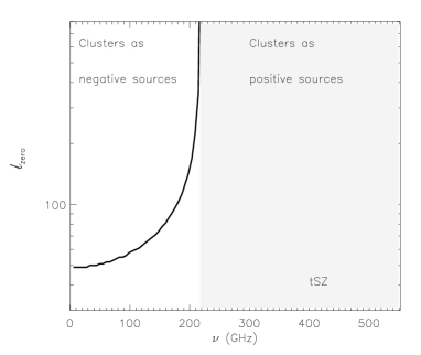
Figure 3: Multipole at which $\delta C_{l}$ induced by the tSZ effect change sigh, for observing frequencies below 218 GHz, for which clusters can be regarded as negative point sources, (Korolev, Syunyaev, & Yakubsev, 1986). Note that it remains constant for RJ frequencies, but shiftes to larger values as $\nu$ tends to 218 GHz. Note, however, that at this frequency the tSZ signal drops to zero.

The different dependence versus $\nu$ for different $l$’s is displayed in Fig.(2): the two extreme cases are given for $\delta C_{l}$ at $l=8$ and $4000$, whereas the intermediate case corresponds to $l=40$. The behaviour of the $\delta C_{l}$’s versus frequency is a consequence of i) the independence of the photon spectrum upon redshift and ii) the fact that the tSZ surface brightness changes sign at $\nu=218$ GHz.

After defining the correlation coefficient as ${\cal R}_{l}\equiv\langle a_{l,m}^{CMB}a_{l,m}^{tSZ}\rangle/\sqrt{C_{l}^{CMB}C_{l}^{tSZ}}$, we plot it for both $\Lambda$CDM and SCDM cosmological models (thick and thin solid lines, respectively), (figure (4)). The ISW is the cause of the coupling of CMB anisotropies with tSZ signal in the $\Lambda$CDM case. This causes a cross-correlation with the total CMB signal of about a 20% at $l\sim 10$, which drops at higher multipoles since the ISW signal decreases rapidly with increasing $l$. For the SCDM model, we obtain $l_{min}\sim 5$ for $\eta_{tSZ}(z\sim 0.5)\sim 6730$ Mpc and $\eta_{0}\sim 8300$ Mpc; and $l_{max}\sim 8$, which would explain the low level of correlation in this case (less than a few percent).

Figure 4: Correlation coefficients ${\cal R}_{l}\equiv\langle a_{l,m}^{CMB}a_{l,m}^{tSZ}\rangle/\sqrt{C_{l}^{CMB}C_{l}^{tSZ}}$ for clusters in the $\Lambda$CDM (thick line) and SCDM (thin line) scenarios.

3.2 Reionization and Resonant Scattering of CMB Photons on Ions, Atoms and Molecules of Heavy Elements

Both scattering on free electrons during reionization and resonant scattering associated to any type of transition in heavy species contribute with some optical depth for the CMB photons. In the first case, the optical depth is generated by the Thompson scattering occuring between CMB photons and free electrons, and, hence, is frequency independent. This situation changes for resonant transitions, provided that CMB photons scatter the line only if their frequency is close enough to the resonant frequency. Apart from this distinction, the effect of both phenomena on the CMB power spectrum is identical, so we shall restrict our analysis on the case of resonant scattering, (which, by its spectral peculiarity, can be separated from the intrinsic CMB temperature fluctuations). Hence, we refer to Basu, Hernández–Monteagudo & Sunyaev (2004), (hereafter BHMS) where this effect is utilized to discuss constraints on the abundances of heavy species at redshifts $0.1<z<30$.

If we denote by $\tau_{rs}$ the homogeneous (i.e. position independent ) optical depth associated to resonant scattering, we can write that the change induced by the resonant transition on the temperature field is given by:

$$T_{rs}=T_{cmb}\;e^{-\tau_{rs}}+T_{gen},$$ (27)

where $T_{rs}$ is the temperature angular fluctuation field at the time of resonant scattering, $T_{cmb}$ is the intrinsic CMB field generated at the LSS and $T_{gen}$ are the new temperature fluctuations generated by the resonantly scattering species. If we now take the limit $\tau_{rs}\ll 1$, the last equation becomes

$$T_{rs}=(1-\tau_{rs})\;T_{cmb}+\tau_{rs}\;T_{gen}^{lin}+{\cal O}[\tau_{rs}^{2}],$$ (28)

with $T_{gen}^{lin}$ the coefficient of the linear term in the expansion of $T_{gen}$ in terms of $\tau_{rs}$. In Fourier space, this translates into:

$$a_{(l,m),\;rs}=(1-\tau_{rs})\;a_{(l,m),\;cmb}\;+\;\tau_{rs}\;a_{(l,m)\;gen}^{lin}$$

$$\phantom{xxxxxxxxxxxxxxxxxxxxxxxxxxxxxxxxx}+\;{\cal O}[\tau_{rs}^{2}],$$ (29)

with $a_{(l,m)}$’s denoting Fourier multipoles. If we now define $\delta C_{l}\equiv\langle|a_{(l,m),\;rs}|^{2}\rangle-\langle|a_{(l,m),\;cmb}|^{2}\rangle$, it is straightforward to find that

$$\delta C_{l}=\tau_{rs}\;2\;\bigl{(}\langle{\cal R}e\;\left[a_{(l,m),\;cmb}\times(a_{(l,m),\;gen}^{lin})^{*}\right]\rangle$$

$$\phantom{xxxxxxxxxxxxxxxxxxx}-\langle|a_{(l,m),\;cmb}|^{2}\rangle\bigr{)}\;+\;{\cal O}[\tau_{rs}^{2}].$$ (30)

As shown in detail in the Appendix A of BHMS, the first term accounts for the correlation between fluctuations generated during recombination and those generated in the epoch of resonant scattering, whereas the second (autocorrelation) term expresses the blurring of the intrinsic anisotropies induced in the LSS due to the resonant scattering at lower redshift; from now this term will be referred to as the blurring term. Note that it is merely proportional to the intrinsic CMB power spectrum at the resonant scattering epoch, and hence, as long as resonant scattering takes place after recombination, the shape of this blurring term will be identical to the primordial CMB power spectrum generated at decoupling, and thus redshift independent. For the reasons outlined at the end of Section 2, the correlation term is only of relevance at the very low $l$ range of multipoles, in which newly generated anisotropies overcome the blurring of original temperature fluctuations and introduces new anisotropy power, (see again Appendix A of BHMS). This occurs for both $\Lambda$CDM and SCDM cosmological models, since the Integrated Sachs-Wolfe effect (hereafter ISW) has no effect here provided that, in adiabatic $\Lambda$ models, it becomes important only at very low redshift, during the $\Lambda$ term dominance, whereas for an Einstein-de Sitter Universe it vanishes in the linear regime, (e.g., Hu & Sugiyama (1995)). Recalling that $\eta_{rec}\sim 300$ Mpc, $\eta_{rs}(z=25)\sim 2811$ Mpc, and that $\eta_{0}\simeq 14000$ Mpc, one finds that $l_{min}\sim 1$ (no drop of the cross correlation expected at low multipoles) and $l_{max}\sim 30$, at which we would expect having some decrease in the amplitude and/or change of sign in the cross correlation. Figure (5) shows the actual computation of the terms in eq. (30): all curves have been computed for $\tau_{rs}=10^{-3}$ and rescaled to $\tau_{rs}=1$, so the actual measurement that our method would provide is then given by the diamonds line times $\tau_{rs}$, (which, for small enough $\tau_{rs}$, is below the cosmic variance limit). As in BHMS, the resonant lines have been modelled by a gaussian centered on the conformal time ($\eta_{rs}$) corresponding to the redshift considered in each case, and with a $\sigma$ equal to one percent of $\eta_{rs}$. Solid lines gives the blurring of the original power spectrum, and the dashed line accounts for the cross-correlation. Note that we are plotting absolute values, and that only at low multipoles the first term is positive and greater in amplitude than the blurring term. For higher multipoles, the correlation term can be neglected and one is left with the simple autocorrelation term:

$$\delta C_{l}\simeq-2\tau_{rs}\;C_{l}^{cmb}.$$ (31)

This $l$-dependence for the $\delta C_{l}$’s is generic for any source of localised optical depth for the CMB photons. This drop in the $\delta C_{l}$’s (and change of sign at some $l_{zero}$, see low $l$ range in figure (5)) are a direct consequence of the correlation of fluctuations at $\eta_{rec},\eta_{rs}$, and provide a test for the origin of the $\delta C_{l}$’s, just as in the case of the tSZ effect addressed above.

Figure 5: Angular power spectrum arising as a consequence of resonant scattering on a line placed at the end of the Dark Ages, ($z=25$). We are plotting the two terms contributing to the total $\delta C_{l}$’s (diamonds): the absoption term is displayed in thick solid line, and is merely proportional to the intrinsic CMB power spectrum. It is negative, and hence the total $\delta C_{l}$’s cross zero only when the Doppler-induced generation (dashed line) becomes relevant at low multipoles. Only absolute values are shown. The correct amplitude of this effect is obtained after multiplying these curves by $\tau_{rs}$.

We remark that these $\delta C_{l}$’s are measurable only if the CMB is being observed at two different frequencies; one corresponding to the resonant scattering at $\eta_{rs}$, and another one in which such resonant scattering can be neglected. Note that there is no place for this situation in the case electron scattering during reionization, since Thompson scattering on free electrons is frequency independent. We are implicitely assuming that the instrument is sensitive to the amplitudes of the $\delta C_{l}$’s: in BHMS we showed that the current detector technology (present in experiments like WMAP, ACT or Planck) should already allow to set strong limits in the abundance of resonant species during the epoch of reionization.

3.3 Emission in Fine Structure Lines of C, N, O in Haloes

BHMS studied the effect of resonant scattering of CMB photons in fine structure transitions associated to metals and ions. They found that very overdense regions ($\delta\geq 10^{4}$) should emit in these lines via collisional excitations, (Suginohara, Suginohara, & Spergel, 1999; Varshalovich, Khersonskii, & Sunyaev, 1981). The expected amplitude of this signal is relatively small, while its spectral dependence is very different from that of the CMB. On the other hand, it also depends on the star formation history in haloes whose large scale distribution should trace the general density fluctuation field. For these reasons, one can consider the application of the correlation method in this case as well. The main difference to the scenario studied by BHMS is that, in this occasion, the scattering in the lines is almost negligible, and hence, no blurring of original CMB anisotropies should be expected. Hence, there will be no further suppresion of the CMB power spectrum at high multipoles, but only extra power in the large angular scale range. This is motivation of an upcoming paper where both the linear and quadratic terms are taken into account.

3.4 Extragalactic Foregrounds

In this subsection we address possible effects that well-known physical processes (such as free-free emission, dust emission in the IGM or inside galaxies and synchrotron emission in extragalactic radio sources) have on our method. In the case of extragalactic foregrounds, it is clear that if they are produced in haloes, they should trace the overall mass distribution in the very large scales, just as in our study of tSZ signal induced by clusters of galaxies. For this reason, one could think of applying this method on them, expecting to find a similar shape for the correlation term at large angular scales as the one found for tSZ clusters. This raises the question whether these foregrounds could mutually contaminate or bias the correlation estimates. Since the method proposed here is based on the frequency dependence of the signal under study, proper frequency coverage should allow to identify and separate each component as long as spectral signatures are distinct enough.

It is obvious that if the sources of these signals are located in our Galaxy, one would not expect any type of correlation between them and the original density perturbation field, leading to no linear ($\propto\epsilon$) term.

4 Discussion and Conclusions

The amplitude of the cross correlation depends essentially on the conformal distance separating the signal sources, rather than the particular $k$ projection of sources of different origin. The closer the sources of the signals are, the higher the correlation becomes. At this respect, the presence of a $\Lambda$ term generating an ISW signal is of crucial importance for those effects generated in our neighborhood, (particularly the tSZ effect, Cooray (2001)). Consistently with the ISW contribution to the total CMB signal (around 20 $\mu$K with respect the total $\sim$ 110 $\mu$K of the CMB), the correlations in a $\Lambda$CDM universe show typical values of 10-20 %, with remarkably lower values in the SCDM scenario. In an Einstein-de Sitter universe, the correlation drops to a few percent, and the enhancement of the weak signal is rather far from being relevant. The situation changes remarkably in the case of resonant scattering at high redshift. In this situation, the correlation coefficient is practically unity for the low multipoles, since, as shown in BHMS, arises as a consequence of the monopole and Doppler terms of the CMB, and the contribution of the ISW component is negligible.

Although the galactic contamination is thought to be more important in the large angular scales where these correlations show up, it is also expected that space experiments achieve their best sensitivities in the big angular scales. In the case that the signal is of extragalactic origin, the cross term will always show up together with the squared term, although both terms have, in general, different frequency (23) and $l$-dependence. This should also help in distinguishing between them, specially in the case of the tSZ effect, for which a peculiar pattern of the $\delta C_{l}$’s versus $l$ and $\nu$ has been predicted. In the high multipole range, frequency dependent scattering such as resonant scattering introduce a measurable blurring of original CMB temperature fluctuations generated during recombination. Since it merely consists in an autocorrelation of CMB anisotropies, this blurring term has the same l-dependence as the original CMB power spectrum.

The method proposed here can also be applied in the study of the cross correlation of CMB temperature fluctuations with the radio background. In the low frequency range, new instruments like the Low Frequency Array (LOFAR) or the Square Kilometer Array (SKA) will measure the radio background. This is mainly due to radio galaxies present in the redshift range $z\in[0,4]$, and its fluctuations are expected to be of much higher amplitude than those of the CMB. However, due to the fact that the radio background is generated by radio galaxies tracing the universal density fluctuation field, one can think of applying this method in order to enhance the CMB component at these frequencies. When doing this, one must keep in mind that there is emission at 21 cm coming from neutral hydrogen during the Dark Ages, ($z\sim(30,100)$, Madau, Meiksin & Rees (1997)) which should fall in this frequency range and which is showing also some degree of correlation with the CMB. However, according to the arguments given in Section 2, most of the correlation will be due to the coupling of the ISW effect with the radio galaxy distribution at low and moderate redshifts.

Similar arguments can be applied when studying the 857 GHz band of Planck’s HFI, since we can expect that this method should be able to unveil the distribution of extragalactic dust and its imprint on the CMB. In other words, by means of the ISW the CMB has become a tool which permits performing independent tests at different frequencies on the large scale distribution of matter. The main two caveats to have present are the possibility of having some signal generated during reionization, at very high redshift, which could be introducing some extra correlation, and the presence of galactic foregrounds, whose residuals might invalidate these analyses in the very low multipoles.

In this paper, we have addressed the issue of correlated signals in the context of CMB. We have shown that, in the case in which two signals have different spectral dependence, the presence of correlations between both can be used in order to enhance the weak signal with respect the dominant one. Assuming that the correlation between signals is caused by the the cosmological density perturbation field, we have found at which angular range such correlation might be relevant. This depends essentially on two different scales: the distance separating the events generating the signals under consideration, and their distance to the observer. In a $\Lambda$CDM universe, these cross terms dominate at the large angular scales, and hence characterize our predictions of the power spectra associated to the weak signals in the low multipole range.

References

- Atrio–Barandela & Mücket (1999) Atrio–Barandela & Mücket, J.P. 1999 ApJ 515, 465
- Banday et al. (1996) Banday, A. J., Gorski, K. M., Bennett, C. L., Hinshaw, G., Kogut, A., & Smoot, G. F. 1996, ApJ 468, L85
- Basu, Hernández-Monteagudo & Sunyaev (2004) Basu, K., Hernández-Monteagudo, C. & Sunyaev, R.A., 2004, A& A 416, 447
- Bennett et al. (2003a) Bennett, C. L. et al. 2003, ApJS, 148, 1
- Bennett et al. (1993) Bennett, C. L., Hinshaw, G., Banday, A., Kogut, A., Wright, E. L., Loewenstein, K., & Cheng, E. S. 1993, ApJ 414, L77
- Bond et al. (2002) Bond, J.R. et al., 2002, astro-ph/0205386
- Boughn & Crittenden (2003) Boughn, S. P. & Crittenden, R. 2004, Nature, 427, 45
- Cooray (2001) Cooray, A. 2001, PhRvD 65, 103510
- Eke, Cole, & Frenk (1996) Eke, V. R., Cole, S., & Frenk, C. S. 1996, MNRAS 282, 263
- Fosalba, Gaztañaga & Castander (2003) Fosalba, P., Gaztañaga, E., & Castander, F. J. 2003, ApJL, 597, L89
- Goldstein et al. (2003) Goldstein, J. H. et al. 2003, ApJ, 599, 773
- Guth (1981) Guth, A. H. 1981, PhRvD, 23, 347
- Hernández-Monteagudo & Rubiño-Martín (2004) Hernández-Monteagudo, C. & Rubiño-Martín, J. A. 2004, MNRAS, 347, 403
- Hu & Sugiyama (1995) Hu, W. & Sugiyama, N. 1995, PhRvD 51, 2599
- Korolev, Syunyaev, & Yakubsev (1986) Korolev, V. A., Syunyaev, R. A., & Yakubtsev, L. A. 1986, Soviet Astronomy Letters, 12, 141
- Kneissl et al. (1997) Kneissl, R., Egger, R., Hasinger, G., Soltan, A. M., & Truemper, J. 1997, A&A, 320, 685
- Komatsu & Kitayama (1999) Komatsu, E. & Kitayama, T. 1999, ApJL 526, L1
- Komatsu & Seljak (2002) Komatsu, E. & Seljak, U. 2002, MNRAS, 336, 1256
- Kosowsky (2003) Kosowsky, A. 2003, New Astronomy Review, 47, 939
- Jenkins et al. (2001) Jenkins, A., Frenk, C. S., White, S. D. M., Colberg, J. M., Cole, S., Evrard, A. E., Couchman, H. M. P., & Yoshida, N. 2001, MNRAS, 321, 372
- Lacey & Cole (1993) Lacey, C. & Cole, S. 1993, MNRAS 262, 627
- Linde (1983) Linde, A. D. 1983, Very Early Universe, 205
- Ma & Bertschinger (1995) Ma, C-P. & Bertschinger, E. 1995, ApJ 455, 7
- Madau, Meiksin & Rees (1997) Madau, P., Meiksin, A., & Rees, M. J. 1997, ApJ, 475, 429
- Mason & CBI Collaboration (2001) Mason, B. & CBI Collaboration 2001, Bulletin of the American Astronomical Society, 33, 1357
- Mo & White (1996) Mo, H. J. & White, S. D. M. 1996, MNRAS 282, 347
- Mukhanov & Chibisov (1982) Mukhanov, V. F. & Chibisov, G. V. 1982, ZhETF, 83, 475
- Press & Schechter (1974) Press, W.H. & Schechter, P. 1974, ApJ 187, 245
- Rubiño-Martín, Atrio-Barandela, & Hernández-Monteagudo (2000) Rubiño-Martín, J. A., Atrio-Barandela, F., & Hernández-Monteagudo, C. 2000, ApJ, 538, 53
- Rubiño–Martín & Sunyaev (2003) Rubiño–Martín, J. A. & Sunyaev, R.A. 2003, MNRAS 345, 221
- Seljak & Zaldarriaga (1996) Seljak, U. & Zaldarriaga, M. 1996, ApJ 469, 437
- Sheth & Tormen (1999) Sheth, R. K. & Tormen, G. 1999, MNRAS, 308, 119
- Smoot et al. (1991) Smoot, G. F. et al. 1991, ApJL, 371, L1
- Springel, White, & Hernsquist (2001) Springel, V., White, M. & Hernsquist, L. 2001 ApJ 549, 681
- Starobinskii (1981) Starobinskii, A. A. 1981, ZhETF Pis ma Redaktsiiu, 34, 460
- Suginohara, Suginohara, & Spergel (1999) Suginohara, M., Suginohara, T., & Spergel, D. N. 1999, ApJ, 512, 547
- Sunyaev & Zel’dovich (1980) Sunyaev, R. A. & Zel’dovich, I. B. 1980, ARA&A, 18, 537
- Varshalovich, Khersonskii, & Sunyaev (1981) Varshalovich, D. A., Khersonskii, V. K., & Sunyaev, R. A. 1981, Astrofizika, 17, 487
- Sunyaev & Zel’dovich (1970) Sunyaev, R. A. & Zel’dovich, I. B. 1970, Ap&SS, 7, 3
- Zeldovich (1972) Zeldovich, Y. B. 1972, MNRAS, 160, 1P
- Zhang, Pen, & Wang (2002) Zhang, P., Pen, U., & Wang, B. 2002, ApJ, 577, 555