Simultaneous Chandra and VLA Observations of Young Stars and Protostars in $\rho$ Ophiuchus Cloud Core A

Abstract

A 96-ks Chandra X-ray observation of $\rho$ Ophiuchus cloud core A detected 87 sources, of which 60 were identified with counterparts at other wavelengths. The X-ray detections include 12 of 14 known classical T Tauri stars (CTTS) in the field, 15 of 17 known weak-lined TTS (WTTS), and 4 of 15 brown dwarf candidates. The X-ray detections are characterized by hard, heavily absorbed emission. Most X-ray detections have visual extinctions in the range A_V $\approx$ 10 - 20 mag, but several sources with visual absorptions as high as A_V $\approx$ 40 - 56 mag were detected. The mean photon energy of a typical source is $\langle$E$\rangle$ $\approx$ 3 keV, and more than half of the detections are variable. Prominent X-ray flares were detected in the unusual close binary system Oph S1, the X-ray bright WTTS DoAr 21, and the brown dwarf candidate GY 31 (M5.5). Time-resolved spectroscopic analysis of the DoAr 21 flare clearly reveals a sequence of secondary flares during the decay phase which may have reheated the plasma. We find that the X-ray luminosity distributions and spectral hardnesses of CTTS and WTTS are similar. We also conclude that the X-ray emission of detected brown-dwarf candidates is less luminous than T Tauri stars, but spectroscopically similar.

Simultaneous multifrequency VLA observations detected 31 radio sources at 6 cm, of which ten were also detected by Chandra. We report new radio detections of the optically invisible IR source WLY 2-11 and the faint H$\alpha$ emission line star Elias 24 (class II). We confirm circular polarization in Oph S1 and report a new detection of circular polarization in DoAr 21. We find no evidence that X-ray and radio luminosities are correlated in the small sample of TTS detected simultaneously with Chandra and the VLA.

We describe a new non-parametric method for estimating X-ray spectral properties from unbinned photon event lists that is applicable to both faint and bright X-ray sources. The method is used to generate $f_{\rm X}$, $\log T$ and $L_{\rm X}$ light curves. In addition, we provide a publically-available electronic database containing multi-wavelength data for 345 known X-ray, IR, and radio sources in the core A region.

1 Introduction

The $\rho$ Ophiuchus cloud is one of the nearest sites of on-going star formation. The optical and infrared study of Chini (1981) gave a mean distance $d$ = 165 $\pm$ 20 pc, but more recent work based on Hipparcos and Tycho data for off-core sources (Knude & Hog, 1998) suggests the value may be as low as 120 pc. We use $d=165$ pc in this paper. Despite its proximity, very few stars are optically revealed due to high extinction. Even so, previous observations at X-ray, near-infrared, far-infrared, and radio wavelengths show a diverse collection of objects including protostars, T Tauri stars, and brown dwarf candidates (BDCs). Near the center of Cloud Core A (as designated by Loren et al. (1990)) are the magnetic B4 star Oph S1 (André et al., 1988, 1991), the Class 0 radio source LFAM 5 (Leous et al., 1991), and the class I protostars GSS 30 IRS-1 and GSS IRS-3, first identified by Grasdalen et al. (1973).

The first X-ray images of $\rho$ Oph obtained with the Einstein Observatory revealed a large population (Montmerle et al., 1983) of flaring young stellar objects (YSOs). In subsequent observations with ROSAT, ASCA, and Chandra, Class I protostars, Class II classical T-Tauri stars, and Class III weak-line T-Tauri stars in $\rho$ Oph have exhibited some of the largest stellar flares ever observed (Koyama et al., 1994; Casanova et al., 1995; Grosso et al., 1997; Kamata et al., 1997; Grosso et al., 2000; Tsuboi et al., 2000; Grosso, 2001; Imanishi, Koyama, & Tsuboi, 2001; Imanishi et al., 2002).

The ubiquity of X-ray flaring and rapid variability suggests that magnetic fields play a central role in the X-ray emission of most young stars. However, the details of this process and the geometry of the magnetic structures involved are still under intense study. Evidence for extended magnetic structures around YSOs comes mainly from high-resolution radio observations. VLA observations have detected moderately circularly polarized nonthermal emission indicative of ordered magnetic fields in WTTS such as Hubble 4 (e.g. Skinner (1993)). At higher angular resolution, VLBI observations have shown that the radio emission of WTTS typically arises in compact regions of diameter $\leq$25 R_∗ with high brightness temperatures T_b $\geq$ 10^7.5 K (e.g., André et al., 1992), (Phillips et al., 1991). Of particular interest here is the strong nonthermal radio source Oph S1 in $\rho$ Oph core A whose magnetospheric diameter $D\approx 12R_{\star}$ has been directly measured using VLBI techniques (André et al., 1991). Oph S1 consists of a magnetic B4 star (Oph S1 A) and a K $=$ 8.3 companion (Oph S1 B) at a separation of 20 mas discovered by lunar occultation (Simon et al., 1995). The B4 star is unusual, belonging to a small class of magnetic OB stars which includes $\theta^{1}$ Ori C (O7 V), the central star of the Orion Nebula.

Although the existence of extended magnetic structures in young stars is now firmly established, it is not yet clear how these magnetic structures relate to the observed X-ray emission (and its variability) nor is it even certain that the emission processes in YSOs are the same as in older late-type stars like the Sun. In the Sun, X-ray emission is ultimately linked to the presence of dynamo-driven magnetic fields. X-ray emitting plasma is confined in magnetic loops and X-ray flares are an observational consequence of rapid energy release during magnetic reconnection events in the corona. However, in younger stars the situation is more complex since magnetic fields may be of primordial origin or produced by dynamo mechanisms that are different from the Sun, and interaction of the stellar magnetosphere and the surrounding disk may be possible.

Shu et al. (1994) and Armitage & Clarke (1996) have invoked extended magnetic fields that couple the photosphere to the disk in order to explain the slow rotation of classical T Tauri stars. If this basic model is correct, then the magnetic fields must extend to the Keplerian co-rotation radius, several stellar radii from the photosphere. Quasi-periodic count rate variations in objects such as the Class I source YLW 15 in $\rho$ Oph core-F (Tsuboi et al., 2000) have been interpreted in terms of differential rotation of the protostar and its accretion disk, leading to magnetic shearing and reconnection thereby producing large-amplitude, long-duration, quasi-periodic X-ray flares (Montmerle et al., 2000). Also, high-resolution Chandra grating spectra of the CTTS TW Hya show weak forbidden-line emission that may be attributed either to high electron densities (Kastner et al., 2002) or to UV irradiation of the X-ray emitting plasma (Gagné et al., 2002), possibly from a UV hot spot. Either explanation suggests that material may be funneled inward along field lines from the inner edge of the disk to the photosphere, producing an X-ray emitting shock at or near the stellar surface.

The possible effects of circumstellar disks and/or accretion on the X-ray emission of young stars is a subject of current interest and debate. The presence of a disk is usually inferred from non-photospheric excesses at near to mid-IR wavelengths. In a Chandra study of the Orion Nebula Cluster (ONC), it was found that stars with and without IR excesses have similar X-ray luminosity functions (Feigelson et al., 2002, 2003). This suggests that IR disks themselves have little if any effect on X-ray emission levels.

However, it is not necessarily the case that all stars surrounded by IR disks are actively accreting, and there is now some evidence that accretion itself (rather than IR disks) may have an effect on X-ray emission. Accreting sources are usually identified by UV excesses or by optical diagnostics such as emission at H$\alpha$, O I, or Ca II. Such optical diagnostics are not generally available in heavily-obscured regions such as $\rho$ Oph, but are accessible in other star-forming regions. The ROSAT surveys of Taurus-Auriga (Stelzer & Neuhäuser, 2001), NGC 2264 and Chameleon I (Flaccomio, Micela, & Sciortino, 2003) and Chandra observations of the Orion Nebula Cluster and IC 348 (Flaccomio et al., 2003; Preibisch & Zinnecker, 2002; Stassun et al., 2004) find that stars with high accretion rates have, on average, 2-3 times lower X-ray luminosity than stars with low accretion rates. Moreover Flaccomio, Micela, & Sciortino (2003) show that, in the Orion Nebula Cluster and in NGC 2264, stars with infrared excesses have lower $L_{\rm X}$ and $L_{\rm X}/L_{\rm bol}$ than stars with no IR excess, although the effect is less pronounced. Flaccomio et al. (2003) argue that accretion and a disk affect the magnetic geometry, thereby reducing the available surface area at the photosphere for closed magnetic loops, thus reducing $L_{\rm X}$ and $L_{\rm X}/L_{\rm bol}$. Flaccomio, Micela, & Sciortino (2003) further suggest that disk dissipation and/or decreased mass accretion causes an increase in $L_{\rm X}/L_{\rm bol}$ during the first few Myrs of PMS evolution. After 10 Myr, $L_{\rm X}/L_{\rm bol}$ declines with rotation.

We present simultaneous observations of the $\rho$ Oph A cloud with the Chandra ACIS-I camera and the VLA that provide new information on the cloud population and its X-ray and radio properties. Our primary objectives were (i) to obtain a sensitive high angular resolution X-ray and radio census of the young stellar population in $\rho$ Oph A and quantify the X-ray and radio properties of the population, (ii) to accurately identify counterparts to X-ray sources at other wavelengths, particularly in the near-infrared and radio, (iii) to determine if significant differences exist in the X-ray properties of the different stellar subgroups (Class 0/I, II, III and brown dwarf candidates), and (iv) to search for possible relationships (including correlated variability) between the X-ray and radio emission of YSOs in $\rho$ Oph A. These simultaneous high-angular resolution X-ray and radio observations are so far unique and provide compelling evidence for strong magnetic activity in the embedded $\rho$ Oph A population.

2 A Database of Young Stellar Objects in $\rho$ Oph A

As part of this study, we have compiled an electronic database consisting of 345 objects in the Chandra ACIS-I FOV. It includes previously cataloged infrared, X-ray, and radio data and visual extinction estimates, as well as new data presented here. All figures and tables herein are based on information in this database. The database is publically available and is described in more detail in Appendix A.

3 Chandra Observation, Data Reduction, and Source Identification

3.1 Chandra Observation and Data Reduction

The Chandra X-ray Observatory observed the $\rho$ Ophiuchus Cloud A (L1688; Lynds, 1962) continuously for 96.5 ks, beginning at 2335 UT on 2000 May 15 and ending at 0319 UT on May 17. Chandra collected consecutive exposures of 3.24 s on the Advanced CCD Imaging Spectrometer (ACIS), using ACIS chips I0-I3 and S2-S3. The ACIS-S chips were located far off-axis and were not used in our analysis, and will not be discussed in this paper. The high-resolution mirror assembly (HRMA) and ACIS-I camera are described in detail in the Chandra Proposers’ Observatory Guide and in Weisskopf et al. (2002). The ACIS I3 aim-point was on Oph S1 at (J2000) $\alpha=16^{\rm h}26^{\rm m}35{\stackrel{{\scriptstyle\rm s}}{{\textstyle{.}}}}2$, $\delta=-24^{\circ}23\arcmin 13\arcsec$.

We applied a standard data reduction using the Chandra Interactive Analysis of Observations software CIAO v2.2.1. The ACIS data were obtained in VFAINT mode, allowing us to remove afterglow events. The event list was filtered to include events with standard ASCA grades and with photon energies in the 0.5-7.0 keV band, thereby significantly reducing the particle background. We checked for background flares and none were found. Source identification (§3.2) and light curve variability analysis (§5.3) are described below. Spectra of selected sources, along with source-specific ARF and RMF response files, were extracted using the CIAO tool PSEXTRACT.

3.2 Chandra Images and Source Identification

Two images which contain the entire 4-CCD ACIS-I FOV were generated to search for X-ray sources: a full-resolution 2800$\times$2800 pixel image ($0.492\arcsec$ pixels) and a binned 1400$\times$1400 pixel image ($0.984\arcsec$ per pixel). Figure 1 shows the full-resolution 2800$\times$2800 pixel image. To register the Chandra image against infrared positions, we selected 43 2MASS sources with obvious counterparts on the Chandra image. The 2MASS J2000 positions and Chandra physical pixel positions were then used to derive a 4-coefficient ACIS-I plate scale solution using the Starlink program ASTROM. The ASTROM $-$ nominal offsets in R.A. and Decl. were $-0.84\arcsec$ and $-3.68\arcsec$, respectively. These offsets were applied to the Chandra image header keywords to obtain the coordinates listed in Table 1.

We detected X-ray sources on each image using CIAO’s wavelet-based tool, WAVDETECT. We ran WAVDETECT using scaling factors 2, 4, and 8, with a false alarm probability of $10^{-5}$. In some cases, regions near the edge of the field of view were detected as sources by WAVDETECT because the off-field background is zero. After visual inspection, these spurious detections were omitted. Two X-ray sources in Table 1 were not detected by WAVDETECT: SKS 3-12=J162622.2-242447 and BKLT J162636-241902=J162636.8-241900. They have been added because they contain more than 7 counts and correspond to known IR sources.

WAVDETECT computes the 1-$\sigma$ major- and minor-axis radii of each source ellipse. Events within a 3-$\sigma$ major- and minor-axis radii ellipse were extracted for each source. In a few cases, the extraction ellipses were shrunk to avoid region overlap with nearby sources. The net counts given in Table 1 are the raw counts in the elliptical extraction region minus the estimated background in the same region. To determine the number of background counts we used the area of the extraction region and assumed a constant 0.5-7 keV background rate over the CCD of 0.17 counts s^-1 per ACIS-I CCD (see the Chandra Proposers’ Observatory Guide). The typical background during our 96.5 ks exposure is approximately 4 counts per source. Table 1 lists the 87 sources in the 17$\arcmin\times 17\arcmin$ ACIS-I FOV. Of the 87 Chandra sources, 60 are identified with catalogued IR or radio sources. All but three of these identifications have X-ray $-$ IR offsets $<1\arcsec$.

4 VLA Observations and Data Reduction

Multifrequency radio observations of $\rho$ Oph core A were obtained simultaneously with Chandra on 2000 May 16 using the NRAO Very Large Array. The observations provided continuous rise-to-set monitoring of $\rho$ Oph over $\sim$7 consecutive hours, as summarized in Table 2. The VLA was in C-configuration and all 26 operational antennas were used at each observing frequency (no subarrays). The primary frequency was 4.86 GHz (6 cm), but briefer coverage was also obtained at 1.42 and 8.46 GHz to search for additional radio sources that might have been missed at 4.86 GHz. Since none were found, the discussion below focuses mainly on the 4.86 GHz results, which provide the best sensitivity and most complete spatial coverage.

Nine separate 6 cm pointings were distributed on a grid centered on Oph S1 with a $\sim 4.5\arcmin$ grid spacing in order to provide nearly uniform radio sensitivity across the full Chandra FOV. Data at each grid point were obtained in two $\sim$15 minute scans, with each scan bracketed by phase calibrator observations. In addition, we obtained a single 1.4 GHz pointing centered on Oph S1 and four 8.4 GHz pointings centered on Oph S1 and the known radio sources LFAM 2, 5, and 15 identified in the previous VLA survey of Leous et al. (1991, hereafter LFAM).

We edited and calibrated the data using the AIPS software package. The data at each grid pointing position were combined to produce separate cleaned maps at each frequency using the AIPS task IMAGR with natural weighting. In those cases where the field contained a bright radio source, we used phase-only self-calibration to improve the dynamic range. Typical rms noise levels at phase center in Stokes I cleaned maps were 36 $\mu$Jy/beam (6 cm), 40 $\mu$Jy/beam (8 GHz), and 220 $\mu$Jy/beam (1.4 GHz). The higher noise level at 1.4 GHz is due mainly to the presence of a bright extragalactic source (BZ6) located $\sim 7\arcmin$ southeast of Oph S1.

4.1 VLA Source Identification

We identified radio sources using cleaned maps at a 5$\sigma$ detection threshold, yielding the 31 detections listed in Table 3. We measured peak fluxes with the AIPS task IMEAN, and we measured total fluxes using IMFIT (Gaussian source model) and TVSTAT (pixel summation inside of the 2$\sigma$ flux contour). Fluxes for off-axis sources were corrected for primary beam attenuation using PBCOR.

Using our database, we attempted to identify known counterparts for each of the radio detections in Table 3. Previous detections at one or more wavelengths were found for 18 of the 31 VLA sources (17 of 28 in the Chandra FOV). Sixteen of the radio sources are confirmations of previous VLA detections obtained by LFAM and Stine et al. (1988, hereafter SFAM). We note that the VLA beam did not resolve Oph S1 A and S1 B. As a result, we assign the radio emission to the binary Oph S1.

We report new radio detections of the IR source WLY 2-11 (J162556.1-243014) and the emission line star Elias 24 ($=$WSB 31$=$J162624.0-241613). WLY 2-11 is an embedded IR source with no visible counterpart and an estimated extinction of $A_{\rm V}=7.3$ (Wilking et al., 1989). Elias 24 is a faint ($R=18.5$) star whose H$\alpha$ emission is barely detectable above the continuum (Wilking et al., 1987). Its spectral type based on near-IR spectra is M2 (Doppmann, Jaffe, & White, 2003).

Two relatively bright 6-cm radio sources observed by LFAM were not detected in our VLA observations: LFAM 20 and LFAM 22 in Table 1 of LFAM, whose respective flux densities in April 1988 were 824 $\mu$Jy and 599 $\mu$Jy. Our upper limits of $\sim$150 $\mu$Jy (3$\sigma$) for these two objects indicate that they have weakened considerably.

Thirteen of the VLA detections have no known counterparts and were not detected in previous VLA surveys of comparable sensitivity (LFAM, SFAM). One of these, J162615.5-243428, is relatively bright with $S_{\rm 6cm}=4.09$ mJy and is offset by $\approx 6\farcs 7$ from the HII region Oph 11. Given that these unidentified sources were not detected previously, some may be variable emitters associated with deeply embedded objects.

5 X-ray Source Properties

5.1 Summary of X-ray Properties

Chandra detected X-ray sources with luminosities spanning more than four orders of magnitude from $\log L_{\rm X}=27.67$ - 31.82 ergs s^-1 (§5.2). The mean photon energy of detections is typically $\langle$E$\rangle$ $\approx$ 3 keV, but the two hardest sources have $\langle$E$\rangle$ $\approx$ 5 keV (Table 1). Variability is detected in 45 of 87 sources (52%) as judged by a value of the Kolmogorov-Smirnov statistic KS $>$ 1 (§5.3). For those detections with known IR counterparts (Table 4), visual absorption ranges from $A_{V}$ = 1.8 - 56.0 mag. The faintest IR source detected by Chandra was GY 144 (K = 13.46).

The list of X-ray detections in Tables 1 and 4 includes 12 of 14 known CTTS and 15 of 17 known WTTS within the ACIS-I FOV. The X-ray luminosity distributions of CTTS and WTTS are similar (§7). Four of 15 BD candidates were detected. Apart from their lower X-ray luminosities, the X-ray properties of BD candidates are otherwise similar to TTS (§9). The class 0 radio source LFAM 5 and the class I protostars GSS 30 IRS-1/IRS-3 were not detected by Chandra, but LFAM 5 and GSS 30 IRS-3 are confirmed as radio sources.

5.2 X-ray Fluxes and Spectral Parameters

The absorbed fluxes in column 8 of Table 1 were computed from the event list of each source, which contains the time-tagged energy of each detected photon. An auxiliary response file (ARF) was generated for each source, which provides the effective area corrected for quantum efficiency (cm² counts photon^-1) versus energy (keV) at the source’s position on the detector. The absorbed X-ray flux at Earth is,

$$f_{\rm X}=\frac{1}{t}\sum_{i=1}^{n}\frac{E_{i}}{a_{i}(E)}-f_{\rm bkg}A,$$ (1)

where $E_{i}$ is the energy of each photon, $a_{i}(E)$ is the corresponding effective area, $t=96439.96$ s is the livetime of the observation, A is the area of the source extraction region, and $f_{\rm bkg}=3.605\times 10^{-18}$ ergs cm^-2 s^-1 pixel^-1 is the 0.5-7.0 keV background flux as determined from a deep, source-subtracted observation from the Chandra calibration database.

Traditionally, extraction and model fitting of a background-subtracted source spectrum are used to determine spectral parameters such as the absorption column density N_H, mean plasma energy kT, and unabsorbed X-ray luminosity L_X. Obviously, an accurate determination of unabsorbed L_X requires knowledge of N_H, as discussed by Casanova et al. (1995). For some sources in $\rho$ Oph, reliable estimates of the visual extinction are available from previous studies, and we are able to constrain the absorption column density using the relation $N_{\rm H}/A_{\rm V}=1.57\times 10^{21}~{}{\rm cm}^{-2}$ mag^-1 (Vuong et al., 2003) (§2). In the absence of A_V information, the X-ray data were used to estimate N_H.

Although the traditional spectral fitting approach gives satisfactory results for bright sources ($\,\stackrel{{\scriptstyle\raisebox{-0.60275pt}{$\textstyle>$}}}{{\sim}}\,$100 counts), it does not work well for fainter sources because of issues related to binning of the spectrum when only a few counts are available. Since $\approx$60% of the X-ray detections in $\rho$ Oph A have $\leq$100 counts, we have developed a non-parametric method for estimating spectral parameters that operates on unbinned photon event data, as described in more detail in Appendix B. This method is based on a large number of simulated isothermal ACIS-I spectra spanning a range of ($\log N_{\rm H}$, $\log T$) values, utilizing the APEC emission model (Smith, Brickhouse, Liedahl, & Raymond, 2001), the Wisconsin absorption model (Morrison & McCammon, 1983), and the MARX ray-tracing Chandra simulation software . The method was used to determine the X-ray temperatures and unabsorbed luminosities for all Chandra detections given in Table 4, as well as N_H values for those detections where a previous determination of A_V was not available. The X-ray temperature and luminosity estimates are based on the assumption that the plasma is isothermal. The inferred values thus provide only a rough temperature estimate that can be used to compare a large number of sources. In reality, the plasma is likely to be more complex, time variable and involve multiple temperature components.

5.3 X-ray Variability and Light Curves

To quantify X-ray variability, the event list of each source was used to calculate the KS statistic, given by

$${\rm KS}=\sqrt{n}\,\sup|f_{i}(t)-f_{0}(t)|.$$ (2)

where $n$ is the number of events, $f_{i}(t)$ is the normalized observed cumulative distribution and $f_{0}(t)$ is the normalized model cumulative distribution, assuming a constant flux. If $z$ is the value of the KS statistic then the null hypothesis probability P($z$), or probability of constant flux, is given by a convergent infinite series (Press et al., 1992):

$${\rm P}(z)=2\sum_{j=1}^{\infty}(-1)^{j-1}e^{-2j^{2}z^{2}}$$ (3)

Truncating the series at six terms gives a few representative values: P(0.5) = 0.96, P(1.0) = 0.27, P(1.5) = 0.02, P(1.7) = 0.006, and P (2.0) = 6.7 $\times$ 10^-4.

Sources with $z$ = ${\rm KS}>1$ generally show some light curve variability and sources with ${\rm KS}>2$ typically reveal obvious signs of flaring. The source event files were used to generate light curves for all 87 X-ray sources. Figures Simultaneous Chandra and VLA Observations of Young Stars and Protostars in $\rho$ Ophiuchus Cloud Core A-Simultaneous Chandra and VLA Observations of Young Stars and Protostars in $\rho$ Ophiuchus Cloud Core A show light curves for seven sources showing interesting variability. The time bin sizes in each light curve are varied so as to include approximately the same number of counts per bin.

The top panel in each light curve shows $f_{\rm X}$, which as already noted is the the background subtracted flux at Earth (Sec. 5.2). In the simplest approximation, $\log T$ and $\log N_{\rm H}$ determine the shape of the X-ray spectrum and the flux conversion factor, the ratio of unabsorbed-to-absorbed flux. At each time bin, $\log T$ and $\log N_{\rm H}$ and their associated random errors are estimated by the non-parametric method described in Appendix B. The two lower panels in Figs. Simultaneous Chandra and VLA Observations of Young Stars and Protostars in $\rho$ Ophiuchus Cloud Core A-Simultaneous Chandra and VLA Observations of Young Stars and Protostars in $\rho$ Ophiuchus Cloud Core A show $\log T$ and unabsorbed luminosity $L_{\rm X}$ assuming a distance $d=165$ pc.

Fig. Simultaneous Chandra and VLA Observations of Young Stars and Protostars in $\rho$ Ophiuchus Cloud Core A reveals that the optically bright WTTS DoAr 21 was in the decay phase of a large flare throughout the observation, and the spectral changes that occurred during this decay are discussed below (Sec. 7.2.3). As apparent in Fig. Simultaneous Chandra and VLA Observations of Young Stars and Protostars in $\rho$ Ophiuchus Cloud Core A, the decay was punctuated by frequent hard-energy spikes, which can be interpreted as reheating events. The peak in mean energy often coincides with or immediately precedes the luminosity peak. The time-resolved spectral fits suggest that the hard-energy spikes are not consistent with sudden increases in column density. As a result, it may necessary to explicitly consider reheating when modeling flare decay with loop models. The relatively short rise and decay times suggest moderate-sized magnetic loops.

5.4 Extragalactic X-ray Sources

The KS statistic, count rate, and $\langle{\rm E}\rangle$ can be used to isolate possible extragalactic X-ray sources (Daniel, Linsky & Gagné, 2002), as demonstrated in Figure Simultaneous Chandra and VLA Observations of Young Stars and Protostars in $\rho$ Ophiuchus Cloud Core Aa-c. Of the 27 Chandra sources with no IR or radio counterparts, 26 show $\langle{\rm E}\rangle>3$ keV, count rates $<0.001$ cts s^-1, and KS$\lesssim 1$. XSPEC simulations of faint, highly absorbed ($25<A_{V}<50$) power-law ($2<\alpha<4$) sources sources give rise to a similar distribution of $\langle{\rm E}\rangle$ and count rate. Furthermore, extragalactic X-ray sources are expected to have low KS statistic because they generally do not show large-amplitude variations on short time scales (Zamorani et al., 1984; Ciliegi & Maccacaro, 1997).

Using equations (2) and (3) of Cowie et al. (2002) to estimate the expected number of extragalactic sources in a 96 ksec exposure of $\rho$ Oph, a limiting flux $f_{\rm X}=9\times 10^{-16}$ ergs cm^-2 s^-1 yields approximately 16 extragalactic sources in the $16\farcm 9\times 16\farcm 9$ ACIS-I FOV. We note, though, that the predicted extragalactic source count depends on the assumed extragalactic source spectrum and the spatially varying absorbing cloud column, both of which are difficult to estimate. Nonetheless, it seems likely that the majority of the 26 Chandra sources with no infrared or radio counterparts are extragalactic. However, a few of the 26 unidentified sources may be new cloud members. In particular, the unidentified Chandra source J162627.4-242418 is a candidate for cloud membership since it is variable in X-rays (KS = 2.77) on a timescale of less than one day.

5.5 X-ray vs. Infrared Properties

Figure Simultaneous Chandra and VLA Observations of Young Stars and Protostars in $\rho$ Ophiuchus Cloud Core A shows a $J-K$ versus $K$ color-magnitude diagram for those IR sources in the ACIS-I FOV with measured JHK magnitudes, including a few fainter sources which have only lower magnitude limits at J. The faintest K-band source detected by Chandra is J162651.9-243039 (= GY 144) at $K=13.46$, although its $J-K$ color is not well-determined.

In Figure Simultaneous Chandra and VLA Observations of Young Stars and Protostars in $\rho$ Ophiuchus Cloud Core A we show a color-color diagram for those IR sources having measured J, H, and K magnitudes. As Fig. Simultaneous Chandra and VLA Observations of Young Stars and Protostars in $\rho$ Ophiuchus Cloud Core A shows, most of the Chandra detections are confined to a strip oriented roughly in the direction of the $A_{V}=10$ reddening vector, consistent with normal reddening for cluster members. The colors of the CTTS GY 81 and the WTTSs SKS 1-11 and GY 84 are consistent with cluster membership but they were not detected with Chandra. We note that the source GY 101 has unusual colors for its assigned class III type, but its J-H value is only a lower limit. We used J $>$ 17.0 (Table 4) to compute its J-H in Fig. Simultaneous Chandra and VLA Observations of Young Stars and Protostars in $\rho$ Ophiuchus Cloud Core A, but 2MASS gives a more stringent limit J $>$ 18.67.

5.5.1 Unclassified Infrared Sources

Chandra detected X-ray emission from more than two dozen IR sources whose SED classifications are not yet known (Table 4). Are these unclassified IR sources cloud members, such as T Tauri stars? We argue below that most of these X-ray/IR sources are not X-ray active AGNs, and conclude that many are likely to be cloud members.

To substantiate the above conclusion, we consider the ratio of X-ray to K-band fluxes. To estimate the unabsorbed IR fluxes, we calculated the interstellar extinction for the J, H, and K bands using

$$\frac{A_{\lambda}}{{\rm E}(J-K)}=2.4\lambda^{1.75}\,{\rm\mu m},$$ (4)

as derived by (Draine, 1989). In conjunction with the fact that,

$$\frac{N_{\rm H}}{{\rm E}(J-K)}=1.1\times 10^{22}\,{\rm cm^{-2}\,mag^{-1}},$$ (5)

(Draine, 1989), we derived $A_{\lambda}$ as a function of known $A_{V}$ for each source. We found that for a typical source ($kT$ $\approx$ 2.0 keV and $N_{\rm H}=3.27\times 10^{22}$ cm^-2), the K band extinction ($f_{\rm K}/f_{\rm K_{\circ}}=0.15$) is similar to the X-ray extinction ($f_{\rm X}/f_{\rm X_{\circ}}=0.25$). Therefore, we used $f_{\rm K}$ to analyze the relationship between IR and X-ray emission. Figure Simultaneous Chandra and VLA Observations of Young Stars and Protostars in $\rho$ Ophiuchus Cloud Core A illustrates that $\log(f_{\rm X}/f_{\rm K})$ is slightly lower for unclassified X-ray/IR sources (median $\log{f_{\rm X}/f_{\rm K}}=-3.0$) than YSOs with measured SEDs (median $\log{f_{\rm X}/f_{\rm K}}=-2.6$). This suggests that most of the unclassified X-ray/IR sources are probably not X-ray active AGN because AGN typically show higher X-ray-to-optical flux ratios than normal stars (Maccacaro et al., 1988; Stocke et al., 1991).

6 Radio Source Properties

6.1 Radio Variability

Each of the VLA detections in Table 3 was observed in two or more $\sim$15 minute scans separated in time by anywhere from $\sim$0.5-3 hours. To search for short-term ($\sim$hours) variability, we compared peak fluxes in the individual scans for the brightest radio detections (S/N$\geq$10).

Definite variability was detected in LFAM 2 (J162622.4-242252) and Oph S1 (J162634.2-242328). The peak 6-cm flux of LFAM 2 increased by a factor of $\sim$5 during the time interval 0629 – 0931 UT, indicative of a radio flare. This radio source is associated with the class III IR source GSS30 IRS-2 (Barsony et al., 1997). No large amplitude flares were detected from Oph S1, but its peak fluxes showed significant scan-to-scan variations of up to $\sim$30% (30$\sigma$) over time intervals of $\sim$3 hours. For example, a 6 cm scan centered on Oph S1 in the time interval 0629 – 0644 UT gave a peak flux $S_{6\rm cm}^{\rm peak}$ = 7.94 $\pm$ 0.06 mJy ($\pm$1$\sigma$) while a second scan at the same pointing position from 0921 – 0931 UT gave $S_{6\rm cm}^{\rm peak}$ = 5.86 $\pm$ 0.08 mJy. Four additional scans with Oph S1 positioned $6\farcm 4$ off-axis also confirm a trend of decreasing radio flux during the observation. Thus, we find for the first time that radio variability is present in this unusual close binary system. We note little or no direct correlation between the VLA and Chandra variability of Oph S1. For example the X-ray flux peak from 0820 – 1005 UT does not coincide with the peak 6-cm emission interval from 0629 – 0644 UT. The apparent decoupling between the X-ray and radio emission is not unique to Oph S1, and has been observed in other PMS objects such as the multiple sytem V773 Tau (Sec. 7.3). If the radio emission is produced in an extended magnetosphere around the B4 star (André et al., 1991) and the X-ray flares are produced in a corona around the K-type secondary, then one would not necessarily expect to see a correlation between the X-ray and radio emission.

Given that the WTTS DoAr 21 was in the decay phase of a large X-ray flare, it is noteworthy that its 6-cm radio flux appeared rather stable. A 15-minute scan centered at 0619 UT with DoAr 21 located $2\farcm 7$ from phase center gave a peak flux of $S^{\rm peak}_{\rm 6cm}$ = 12.04 $\pm$ 0.05 mJy, and a second 10-minute scan at the same pointing position centered at 0939 UT gave $S^{\rm peak}_{\rm 6cm}$ = 11.82 $\pm$ 0.04 mJy. Two additional scans centered at 0542 UT and 1007 UT with DoAr 21 located $7\farcm 7$ from phase center also gave peak fluxes differing by less than 3$\sigma$. Thus, we find no compelling evidence for radio variability in DoAr 21 up to the end of the last VLA 6 cm scan at 1013 UT, but no simultaneous radio coverage is available during the last $\sim$16 hours of the Chandra observation when several X-ray temperature spikes occurred (Fig. 2). Even though no 6 cm variability was detected, DoAr 21 is clearly variable on longer timescales. The 6 cm fluxes quoted above are between the peak flare value of 46.1 mJy on 1983 February 18 and the much lower level of 3.7 mJy measured on 1983 June 18 (Stine et al., 1988).

6.2 Circular Polarization

Circularly polarized radio emission indicative of nonthermal processes was clearly detected at 6 cm in three sources. These are the optically visible G-K type star DoAr 21 (J162603.0-242336), Oph S1 (J162634.2-242328), and the extragalactic source LFAM 21$=$BZ6 (J162700.0-242640). The fractional circular polarization ($\pi_{c}=$V/I) and detection significance (S/N ratio) for these sources are given in the notes to Table 3.

Previous detections of circular polarization in Oph S1 at both 6 cm and 2 cm (with an upper limit at 20 cm) were reported by André et al. (1988). We confirm the presence of circular polarization at 6 cm and also provide a new detection at 3.5 cm, but likewise fail to detect circular polarization at 20 cm.

7 Discussion: The Young Stellar Population in $\rho$ Oph A

7.1 Class 0/I Protostars

The core-A region contains three well-known protostars, namely the class 0 source LFAM 5 and the class I sources GSS30-IRS1 and GSS30-IRS3. In many respects, LFAM 5 is the most unusual of the three. It is a centimeter radio source that is thought to be driving a molecular outflow (André et al., 1990), but has so far not been detected at millimeter, IR, or X-ray wavelengths. Our VLA observation confirms radio emission from LFAM 5 (Table 3) at a 6 cm flux density similar to that reported by LFAM.

GSS30 is an asymmetric infrared bipolar reflection nebula with at least 3 IR sources seen in projection (Grasdalen et al., 1973; Castelaz et al., 1985; Weintraub et al., 1993). The class I source GSS30-IRS1 is thought to be the illuminating star (Castelaz et al., 1985). It has not been previously detected at centimeter radio wavelengths and we likewise obtain only an upper limit of S_6cm $\leq$ 0.12 mJy (3$\sigma$) and an identical upper limit at 3.5 cm. Observations at 2.7 mm have also failed to detect GSS30-IRS1 (Zhang, Wootten, & Ho, 1997). There is no confirmed detectable outflow in this source. However, line emission in recent VLT IR spectra was interpreted as possible evidence for dense gas in an accretion shock (Pontoppidan et al., 2002).

The class I source GSS30-IRS3 has K = 12.85 but no emission peak is seen at J or H (Weintraub et al., 1993), and is thus much fainter than IRS1. A 2.7 mm continuum source has been detected toward GSS30-IRS3 at S_2.7mm = 29 mJy (Zhang, Wootten, & Ho, 1997). Centimeter radio emission is also detected from the radio source LFAM 1, which is identified with GSS30-IRS3. We confirm radio emission from LFAM 1 (Table 3) at a 6 cm flux near the value reported by LFAM.

None of the three class 0/I sources discussed above was detected in our Chandra observation. Upper limits (Table 5) suggest that their luminosities are below $\log L_{\rm X}\approx 28.5$ ergs s^-1. However, these upper limits are based on uncertain $A_{V}$ and $kT$. In the absence of specific information, we have assumed $kT\approx 2.5$ keV and $\log N_{\rm H}\approx 22.5$ cm^-2, typical of X-ray detected TTS in core A. An extinction estimate $A_{V}$ $\approx$ 38 is available for GSS30-IRS1 (Castelaz et al., 1985), and using this value along with $kT\approx 2.5$ keV and a 7 count Chandra detection threshold we obtain $\log L_{\rm X}\leq 28.4$ ergs s^-1 (0.5 - 7 keV). Assuming a higher temperature $kT\approx 6$ keV, as measured for two class I sources in the cluster IC 348 (Preibisch & Zinnecker, 2002), then the upper limit for GSS30-IRS1 becomes $\log L_{\rm X}\leq 28.2$ ergs s^-1.

We thus conclude that the X-ray luminosities of GSS30-IRS1 (and also very likely GSS30-IRS3) are well below the value of $L_{\rm X}\approx 10^{30}$ ergs s^-1, typical of class I sources detected by Chandra such as those in IC 348 (Preibisch & Zinnecker, 2002) and $\rho$ Oph core-F (Imanishi, Koyama, & Tsuboi, 2001). However, the radio luminosities of both LFAM 5 and GSS30-IRS3 are comparable to those of CTTS detected in core A (Sec. 7.2.2). Several factors may influence the X-ray detectability of class 0/I sources. Most importantly, variability seems to be a factor since several of the class I objects detected by Imanishi, Koyama, & Tsuboi (2001) in core F were caught during X-ray flares. Extinction also plays a role, and class 0 objects in particular are believed to have very high absorption that efficiently masks any soft X-ray emission that is present. Extinction will also make it more difficult to arrive at a complete picture of X-ray production mechanisms in protostars. GSS30 IRS1 is a case in point. The suggestion that an accretion shock is present (Pontoppidan et al., 2002) raises the possibility that soft X-rays may be produced in the shock region, similar to what may be occurring in the CTTS TW Hya (Kastner et al., 2002). Since shock-induced X-rays are expected to have characteristic temperatures below $\sim$1 keV, such emission (if present) would be heavily absorbed and difficult to detect in protostars with typical extinctions $A_{V}\approx 40$.

7.2 T Tauri Stars

7.2.1 X-ray Luminosity Functions

Using the unabsorbed $L_{\rm X}$ values of X-ray detections (Table 4), the median X-ray luminosity of the 12 detected CTTS is $\log L_{\rm X}=29.92$ ergs s^-1 which is similar to the median for 15 detected WTTS of $\log L_{\rm X}=29.79$ ergs s^-1. To make further comparisons between the X-ray luminosities of CTTS and WTTS, we take X-ray upper limits of the undetected TTS into account (Table 5). Including both detections and non-detections, all four versions of the generalized Wilcoxon test in the ASURV statistical analysis package (Lavalley et al., 1992) give a probability $p$ = 0.53 that the CTTS and WTTS X-ray luminosities are drawn from the same distribution. Thus, the Wilcoxon test is inconclusive for this sample. Even so, the the Kaplan-Meier estimators for the CTTS and WTTS samples shown in Figure Simultaneous Chandra and VLA Observations of Young Stars and Protostars in $\rho$ Ophiuchus Cloud Core A appear very similar, agreeing to within the error bars.

We also find that the spectral hardnesses in CTTS and WTTS are nearly identical. Using the mean photon energies $\langle$E$\rangle$ in Table 1, the CTTS detections have median $\langle$E$\rangle$ = 2.57 and WTTS detections have median $\langle$E$\rangle$ = 2.53.

On the basis of the shapes of their IR spectral energy distributions, CTTS (class II sources) are thought to be surrounded by circumstellar disks but WTTS (class III sources ) are not. Given that the X-ray luminosities and spectral hardnesses of the CTTS and WTTS in our sample are quite similar, there is no compelling evidence that the presence or absence of infrared disks has any significant effect on their X-ray emission. However, it should be emphasized that accretion diagnostics (like H$\alpha$ or Ca II emission) are not generally available for sources in $\rho$ Oph cloud core A. Thus, our results cannot be used to determine whether accretion itself affects the X-ray properties of this small sample.

7.2.2 Radio vs. X-ray Luminosities

Figure Simultaneous Chandra and VLA Observations of Young Stars and Protostars in $\rho$ Ophiuchus Cloud Core A shows the 5 GHz radio luminosities ($L_{\rm 6cm}$) and X-ray luminosities ($L_{\rm X}$) for those 6 TTS (class II and III) that were simultaneously detected with the VLA and Chandra, along with Chandra upper limits for class 0/I sources. We have also included Oph S1, whose IR classification is uncertain because of the close binary separation. Even though the sample is small, we have checked for a correlation between $L_{\rm 6cm}$ and $L_{\rm X}$ amongst TTS. Excluding Oph S1, the generalized Kendall’s tau test in the ASURV software package gives a correlation probability $p$ = 0.15 and the Cox proportional hazard model gives $p$ = 0.64. If Oph S1 is included (on the suspicion that its faint companion Oph S1B is a TTS), then these values increase slightly to $p$ = 0.35 and $p$ = 0.81, respectively. Thus, we find that radio and X-ray luminosity are not strongly correlated in this small sample of detected TTS.

We do note however that in our small sample there is a tendency for WTTS to be more luminous radio sources than CTTS, even when comparing objects with similar $L_{\rm X}$. In Table 3, all four WTTS (class III) have larger $L_{\rm 6cm}$ values than the two CTTS (class II). This may reflect different radio emission processes in WTTS and CTTS, with nonthermal emission being more common in WTTS. It can also be seen from Figure Simultaneous Chandra and VLA Observations of Young Stars and Protostars in $\rho$ Ophiuchus Cloud Core A that Oph S1 is clearly situated in the region of higher $L_{\rm 6cm}$ occupied by WTTS.

Two objects of some interest are the class II sources Elias 24 (J162624.0-241613) and GY51 (J162630.5-242256), both of which were detected simultaneously with Chandra and the VLA. As Figure Simultaneous Chandra and VLA Observations of Young Stars and Protostars in $\rho$ Ophiuchus Cloud Core A shows, they have similar $L_{\rm X}$, but GY 51 is nearly an order of magnitude more luminous in the radio. GY 51 shows a weak X-ray flare near 1115 UT on May 16, while Elias 24 experienced a moderately strong impulsive X-ray flare near 2400 UT. The 3.6 cm and 6 cm radio fluxes of GY 51 are nearly identical, suggesting a flat (or non-rising) spectral energy distribution and possible non-thermal radio emission.

The faint M2 star Elias 24 was only detected at 6 cm, so no definitive estimate of its radio spectral index is available. However, there is no significant 3.6 cm emission in a scan with Elias 24 positioned 6.6^′ from phase center, and we obtain an upper limit S_3.6cm $\leq$ 0.2 mJy (5$\sigma$). This upper limit is approximately equal to the measured flux at 6 cm (Table 3), suggesting a non-positive spectral index $\alpha$ $\leq$ 0 (S_ν $\propto$ $\nu^{\alpha}$). This may be an indication of nonthermal emission from magnetically-trapped particles. Such emission would be consistent with the impulsive X-ray variability, which is an indicator of magnetic activity. However, the radio interpretion is not yet clear since Gómez et al. (2003) have identified Elias 24 as the possible driving source of a near-IR knot located 144^′′ away. If this identification is correct, then the 6 cm radio emission could be thermal emission associated with an outflow, as is already known to occur in other sources associated with Herbig-Haro objects (Bieging, Cohen, & Schwartz, 1984). Higher sensitivity multi-wavelength observations will be needed to determine if the newly-detected radio emission of Elias 24 is thermal or nonthermal.

7.2.3 Time-Resolved X-ray Spectroscopy of a Large Flare on DoAr 21

DoAr 21=GSS 23=V2246 Oph (K1, WTTS) is the brightest X-ray source in the ACIS-I FOV. As is evident in Fig. Simultaneous Chandra and VLA Observations of Young Stars and Protostars in $\rho$ Ophiuchus Cloud Core A, DoAr 21 was in the decay phase of a large flare throughout the Chandra observation. DoAr 21 was placed far off-axis to migitate pile-up in the ACIS I3 CCD. Although the total count rate of DoAr 21 exceeded 1 counts s^-1 at the beginning of the observation, the source did not pile up significantly, contrary to a previous claim by Imanishi et al. (2002). We find that the pileup fraction never exceeded a few percent because the maximum count rate in the central pixel of the PSF was 0.015 counts s^-1 pixel^-1. Although the count rate decay in the top panel appears to be quite smooth up to a small flare around day 0.8, the $\log T$ light curve in the second panel is variable throughout. We note that the temperature spikes appear to signal reheating events. In many cases, a temperature spike immediately precedes a $f_{\rm X}$ maximum. Based on its V-band absorption (Wilking et al., 2001), we expect DoAr 21 to have a column density $N_{\rm H}\approx 1.0\times 10^{22}$ cm^-2. $\log T$ and $L_{\rm X}$ in each time bin were estimated using the non-parametric method in Appendix B.

In order to confirm the validity of the light curve analysis, the $\sim$81000 counts associated with DoAr 21 were divided into 41 time segments each containing approximately 2000 counts. For each of the 41 ACIS-I spectra, background spectra and response files were generated using the CIAO tool PSEXTRACT. Each of these were modeled in XSPEC V11 using a single-temperature VAPEC model. We generally found good fits ($\chi^{2}\lesssim 1$) using an Fe abundance of 0.5 solar and a column density $N_{\rm H}\approx 1.0\times 10^{22}{\rm cm}^{-2}$. Because column-density variations have been reported during X-ray flares on YSOs (Tsuboi et al., 1998), the column density, temperature, and normalization were free parameters. After each fit, the emission measure and absorption-corrected X-ray luminosity were calculated assuming a distance of 165 pc (Chini, 1981). Indeed, apparent variations of 10–20% in the best-fit column density values are seen throughout the observation. The increases in $N_{\rm H}$ do not generally show corresponding increases in hardness ratio or count rate. The increases in best-fit $N_{\rm H}$ are, however, associated with decreases in the best-fit temperature and increases in $L_{\rm X}$ as a result of the increased correction due to absorption. We believe that this result is an artifact of the fitting procedure: moderate-resolution, moderate signal-to-noise spectra cannot distinguish small increases in column density from small increases in temperature. Since we have no reason to suspect large column-density changes on a WTTS like DoAr 21, the column-density was fixed at the median best-fit value: $N_{\rm H}=1.08\times 10^{22}{\rm cm}^{-2}$ and the spectra were then refit. Note that this value of $N_{\rm H}$ determined from spectral fits differs by only 6% from the value determined by our non-parametric analysis (Table 4).

Assuming $V=13.62$, ${\rm BC}=-0.36$, $d=165$ pc, $N_{\rm H}=1.08\times 10^{22}{\rm cm}^{-2}$, and $N_{\rm H}/A_{\rm V}=1.57\times 10^{21}~{}{\rm cm}^{-2}$ mag^-1, the bolometric luminosity of DoAr 21 is $L_{\rm bol}\approx 2.3\times 10^{35}$ ergs s^-1. During the Chandra observation, $L_{\rm X}/L_{\rm bol}$ decreases from $4.0\times 10^{-4}$ to $2.2\times 10^{-4}$.

The results of the time-resolved spectral analysis are shown in Fig. 2. There is a steady overall decline in emission measure and $L_{\rm X}$ over the course of the observation and the plasma undergoes no fewer than five temperature spikes. If the temperature spikes are ignored, then the plasma would appear to be cooling slowly from a giant flare which occurred before the start of the Chandra observation. The long decay time and the slow but steady decrease in temperature would indicate a large, low-density flaring loop. For example, the two-ribbon flare model of Kopp & Poletto (1993) implies a loop radius in the range $1-3R_{\odot}$.

Previous observations of DoAr 21 with ROSAT and ASCA suggest approximately one large flare per day (Imanishi et al., 2002). If the flare decay in Fig. 2 is typical of flares on DoAr 21, then the corona is in a state of nearly continous flaring with low- and moderate-energy flares outnumbering large flares.

The frequent increases in $kT$ seen in Fig. Simultaneous Chandra and VLA Observations of Young Stars and Protostars in $\rho$ Ophiuchus Cloud Core A suggest that plasma is being intermittently reheated by moderate-energy flares. If the reheating events occurred in the same loops as the primary decaying flare then a simple cooling-loop model will significantly overestimate the cooling time, thereby underestimating the density and overestimating the loop radius. Or, the smaller flares may signal reconnection events in separate magnetic loops.

Long, uninterrupted monitoring of DoAr 21 or simliar stars may provide a clue to the location of these smaller, shorter-duration flares. If short-duration flares during the decay phase of long-duration flares are more frequent than short-duration flares during “quiescent” periods, then the two types of flares probably occur in the same or adjoining arcades of magnetic loops.

A final question concerns the geometrical relationship between the X-ray and radio emitting regions in DoAr 21. As already noted (Sec. 6.1), two separate VLA scans of DoAr 21 at 0619 UT and 0939 UT (16 May) gave nearly identical 6 cm fluxes differing by $<$2%, while at the same time its X-ray flux declined by about 15%. This indicates that the circularly polarized nonthermal radio emission originating in large magnetospheric structures is effectively decoupled from the thermal X-ray emission, which originates much closer to the star - presumably in hot coronal plasma. Similar behavior was noted by Feigelson et al. (1994) in simultaneous ROSAT and VLA/VLBI observations of the unusual WTTS V773 Tau. However, the radio flux of V773 Tau declined while its X-ray emission remained steady, whereas the opposite behavior is observed in DoAr 21. The interpretation of the behavior of V773 Tau is now complicated by the discovery that it is a quadruple system consisting of a K2V + K5V spectroscopic binary with a nearby M-dwarf at 0.12^′′ (Ghez et al., 1995), and an IR companion 0.21^′′ away (Duchene, Ghez, & McCabe, 2001). ROSAT could not spatially resolve these four components, raising the obvious question of whether the (variable) radio emission and (steady) X-ray emission originated in the same star. Even though DoAr 21 is not yet known to be such a closely-spaced multiple system, this possibility should not yet be dismissed given its similarities to V773 Tau.

7.3 The Unusual Close Binary System Oph S1

Figure 15 shows the ACIS-I spectrum of the unusual magnetically-active binary system Oph S1. As we have noted, this star consists of a B-type primary and a fainter secondary at 20 mas separation (Simon et al., 1995). At this close separation, the two components cannot be spatially resolved by Chandra or the VLA. The spectrum shows strong absorption with little or no detectable emission below $\sim$1 keV. There are no clearly discernible emission line features in the spectrum. The light curve shown in Fig. Simultaneous Chandra and VLA Observations of Young Stars and Protostars in $\rho$ Ophiuchus Cloud Core A shows $L_{\rm X}$ variations from $2-4\times 10^{30}$ ergs s^-1 with two small flare peaks at 0815 UT and 2453 UT.

We have analyzed the spectrum using a variety of emission models in XSPEC including single-temperature (1T) and two-temperature (2T) optically thin plasmas (VAPEC), bremsstrahlung, power-law (PL), and the Chebyshev polynomial differential emission measure (DEM) model C6PVMKL. All models included an absorption component and the spectrum was rebinned to a minimum of 15 counts per bin prior to fitting in XSPEC. We compared spectral fits using spectra extracted with CIAO v. 2.2.1 and with the more recent CIAO v. 2.3/CALDB 2.0. and CIAO v 3.0.2/CALDB 2.26 releases. Corrections for charge transfer inefficiency (CTI) were applied to the spectra extracted with CIAO v. 2.3 and CIAO v 3.0.2. The best-fit values from spectral fits in Table 6 are from CIAO v. 2.3 with CTI corrections applied. Generally, the three different versions of CIAO gave similar best-fit values but the fit residuals as measured by reduced $\chi^{2}$ were 15% - 20% smaller with CTI corrections applied.

Because of the lack of strong emission features, several different models can acceptably fit the Oph S1 spectrum. Table 6 gives the derived spectral parameters for a power-law model as well as 1T and 2T VAPEC models. As can be seen, the fit statistics are very similar for these three models. Thus, we cannot distinguish between a power-law spectrum and optically thin plasma emission at the signal-to-noise ratio of the Oph S1 X-ray data.

The 1T VAPEC model implies a mean plasma temperature kT $\approx$ 2.4 keV. A bremsstrahlung model gives a nearly identical temperature kT $\approx$ 2.1 keV and the C6PVMKL model also shows a strong emission measure peak at kT $\approx$ 2.0 - 2.4 keV. Considered collectively, these models indicate that most of the emission arises from plasma at or slightly above kT $\approx$ 2 keV (T $\approx$ 2.3 MK), assuming a thermal origin.

A 1T VAPEC model using solar abundances gives a relatively poor fit ($\chi^{2}$/dof = 165.4/135 = 1.23). The fit can be substantially improved by allowing the Fe abundance to vary. As Table 6 shows, the inferred Fe abundance is quite low, amounting to only a few tenths of the solar value. Little or no further improvement was obtained by allowing the abundances of other elements (Ne, Mg, Si, S) to vary. We thus conclude that if the emission is thermal then the iron abundance is well below solar.

All models give an absorbed flux $\log f_{\rm X}=-12.52$ ergs cm^-2 s^-1 (0.5 - 7 keV) and an absorption column density near log N_H = 22.27 cm^-2. The 1T and 2T VAPEC models (Table 6) give unabsorbed luminosities in the range log L_X = 30.37 - 30.59 ergs s^-1 (0.5 - 7 keV) at d = 165 pc. The above values are in very good agreement with those derived using the independent non-parametric approach (Tables 1 and 4; Appendix B).

The temperature range deduced from VAPEC models of Oph S1 is similar to that seen in T Tauri stars. The X-ray luminosity of Oph S1 is somewhat higher than the median value for TTS detected in core A, but still within the observed range for TTS. Thus, most of the X-ray emission could be produced by the faint companion star Oph S1 B discovered by lunar occultation.

7.4 Brown Dwarf Candidates

Chandra detected 4 of 15 known brown dwarf candidates (BDCs) in core A, namely GY 5 (spectral type M7), GY 31 (M5.5), GY 37 (M6) and GY 59 (M6) (Wilking et al., 1999). As a class, these objects are very weak X-ray emitters. The median luminosity of the four BDC detections is $\log L_{\rm X}=28.3$ ergs s^-1, which is a factor of $\sim$50 below the median $L_{\rm X}$ for TTS detected in core A. Assuming a detection threshold of 7 counts, the 11 undetected BDCs have upper limits $\log L_{\rm X}\leq 27.80$ ergs s^-1. Using the bolometric luminosities of Wilking et al. (1999), the four detected BDCs have $\log L_{\rm X}/L_{\rm bol}$ in the range $-4.71$ to $-3.46$, where the latter value is for the flare source GY 31. Brown dwarfs in other star-forming regions exhibit similar X-ray activity levels (Imanishi et al., 2002; Preibisch & Zinnecker, 2002; Feigelson et al., 2002; Mokler & Stelzer, 2002).

In addition to their faint X-ray emission, the BDCs in core A are also undetected in our VLA observations. Typical radio upper limits for X-ray detected BDCs are $S_{\rm 6cm}$ $\leq$ 0.16 mJy or $L_{\rm 6cm}$ $\leq$ 15.7 ergs s^-1 Hz^-1.

Apart from their faint $L_{\rm X}$, the X-ray properties of detected BDCs appear to be similar to TTS. The median value of mean photon energy for the detected BDCs is $\langle$E$\rangle$ = 2.3 keV, only slightly lower than the median of 2.5 keV for TTS (§7.2.1). Strong variability in the form of a flare was detected in one BDC (GY 31), as discussed below. Thus, GY 31 has a larger X-ray to K-band flux ratio $f_{X}$/$f_{K}$ than most TTS, but the other 3 BDCs which did not flare have $f_{X}$/$f_{K}$ similar to TTS (Table 4).

Figure Simultaneous Chandra and VLA Observations of Young Stars and Protostars in $\rho$ Ophiuchus Cloud Core A shows the flaring light curve of GY 31. The flux declined by a factor of $\sim 5$ during the first 10 ksec of the observation. The hard-band light curve (not shown) closely tracks the broad-band behavior, but there is very little emission in the soft-band below 2 keV due to strong absorption.

We attempted to fit the time-averaged spectrum of GY 31 (Figure Simultaneous Chandra and VLA Observations of Young Stars and Protostars in $\rho$ Ophiuchus Cloud Core A) using optically thin plasma models as well as bremsstrahlung and power-law models. These different models give nearly identical reduced $\chi^{2}$ values and we conclude that there are insufficient counts ($\approx$380 counts) to reliably distinguish between optically thin plasma emission and other alternatives. All models give a high absorption column density log N_H (cm^-2) = 22.76 $\pm$ 0.08. Equating this to a visual extinction (Vuong et al., 2003) yields A_V $=$ 37 mag. Thus, this object is viewed through very heavy absorption, as also determined from infrared observations (Wilking et al., 1999).

If the emission is assumed to originate in an optically thin plasma as is usually the case for TTS, then 1T VAPEC fits using a subsolar Fe abundance in the range Fe = 0.3 - 0.5 solar give $kT=2.3$ [1.6 - 2.9] keV. Due to the high absorption, 2T models with a cooler component give no significant improvement over 1T models. This time-averaged temperature structure is similar to that found in TTS in our sample.

8 Summary

We report new results based on simultaneous X-ray and radio continuum observations of $\rho$ Oph cloud core A using Chandra and the VLA. The most important findings of this study are the following:

1. Chandra detected 87 X-ray sources, of which 60 have known infrared or radio counterparts. At least 16 of the 26 unidentified Chandra sources are suspected to be extragalactic. More than one-half of the X-ray detections showed variability, and the X-ray sources are typically hard and heavily absorbed ($\langle$E$\rangle\approx 3$ keV, $A_{V}$ $\approx$ 2 - 56 mag).

2. Chandra detected 12 of 14 known CTTSs and 15 of 17 WTTSs in $\rho$ Oph core A. Their X-ray luminosities and spectral characteristics are similar, and we thus find no compelling evidence that the presence or absence of circumstellar disks (as discerned from IR excesses) has any significant effect on their X-ray emission. The effects (if any) of accretion on the X-ray emission in this small TTS sample are not yet known due to the lack of suitable (e.g. optical) accretion diagnostics.

3. None of the three class 0/I protostellar sources in core A was detected by Chandra with upper limits at $\log L_{X}\raisebox{-2.58334pt}{$\,\stackrel{{\scriptstyle\raisebox{-0.60275pt}{$\textstyle<$}}}{{\sim}}\,$}28$ ergs s^-1. A comparison with X-ray detections of class I sources in other star-forming regions suggests that such protostars are preferentially detected during periods of enhanced X-ray emission (flares). Our data indicate that in the absence of flares, X-ray luminosities can be one to two orders of magnitude below the typical value $\log L_{\rm X}\sim 30$ ergs s^-1 reported for flaring class 0/I sources.

4. Chandra detected 4 of 15 known brown dwarf candidates in core A, including the flaring source GY 31. Their X-ray emission is faint with a median $\log L_{\rm X}=28.3$ ergs s^-1 that is a factor of $\sim$50 lower than T Tauri stars in core A. The mean X-ray energies and variability of BDCs appear to be similar to TTS. None of the X-ray emitting BDCs was detected with the VLA.

5. The WTTS DoAr 21 was in the decay phase of a large X-ray flare during the Chandra observation, but no radio variablity was detected. Time-resolved X-ray spectroscopy reveals multiple secondary flares during the decay. These secondary flares are associated with temperature increases, suggesting that the plasma is being reheated if the secondary events occur in the primary flaring structure. Such reheating could contribute to the long decay times seen in some large YSO X-ray flares.

6. The X-ray light curve of the binary Oph S1 shows hot, moderate-amplitude, short-duration flares typically seen on TTSs. Much of the X-ray emission may be produced around the K-type secondary located 20 mas from the B4 primary. It remains to be determined whether the variable radio emission originates in a magnetosphere around the B4 star or is instead due to the nearby late-type companion.

7. Multifrequency VLA observations detected 31 radio sources in $\rho$ Oph core A, of which 16 are confirmations of previous radio detections. New radio detections are reported for the emission-line star Elias 24 and the optically invisible IR source WLY 2-11, as well as the first detection of circular polarization in the radio-bright WTTS DoAr 21. There is no significant correlation between the X-ray and radio luminosities in the small sample of T Tauri stars detected simultaneously with Chandra and the VLA.

Appendix A Electronic Database of Objects in $\rho$ Oph Core A

The $\rho$ Oph A region has been studied extensively in most regions of the spectrum and a large amount of observational data exist. In order to make comparisons between the new Chandra and VLA data and existing data, we used IDL to construct a database of the cataloged infrared (Barsony et al., 1997; Bontemps et al., 2001; Allen et al., 2002, 2MASS), X-ray (Casanova et al., 1995; Grosso et al., 2000) and radio sources (Stine et al., 1988; Leous et al., 1991) in the Chandra FOV. We matched sources which fell within the combined positional uncertainty published for each source. We visually checked every match using the ds9 tool in CIAO and against the alternative associations determined by the author of each catalog. Similarly, the measured photometry of each source was also checked for consistency. We omitted two sources from the 2MASS catalog as they had no counterparts and appeared to be reflection nebulae in the 2MASS images.

We used the findings of Simon et al. (1995), who performed a search for binaries by lunar occultation. Their study included the portion of $\rho$ Oph discussed in this paper. Three binary systems, Oph S1, DoAr 24E, and Elias 30, are in the Chandra FOV. In our database, all information previously associated with Oph S1 is assigned to Oph S1 A. We assign the same V-magnitude absorption ($A_{\rm V}$) and column density ($N_{\rm H}$) to both Oph S1 A and Oph S1 B. We associate all Chandra X-ray emission with Oph S1 B (see §7.3). Because of the close 20 mas separation of Oph S1 A and Oph S1 B, some caution is needed when attributing emission to either of the two components. Any further determinations of the origin of cataloged emission for Oph S1 are at the discretion of the user of the data base. We also associate the Chandra X-ray emission in the region of DoAr 24E with the binary companion, DoAr 24E B. We use the IR photometry determined by Allen et al. (2002) for this source. All other cataloged information is assigned to DoAr 24E A in this database. The user should be aware that the IR photometry measurements for DoAr 24E A are likely combined in the IR catalogs. Elias 30 is separated in Barsony et al. (1997), and we use their catalog for the IR photometry. We use the K-band magnitudes derived by Simon et al. (1995) for each of these six sources.

A total of 318 previously cataloged objects exist in the Chandra ACIS-I FOV. In our observations we add 27 new objects detected with Chandra, one of which (J162607.3-242530) was simultaneously detected with the VLA (see §4.2). We matched these 345 sources with known brown dwarf (BD) candidates (Neuhäuser et al., 1999; Wilking et al., 1999), spectral types (Martín et al., 1998; Wilking et al., 1999, 2001), and classification designations based on studies of spectral energy distributions (SEDs), using classifications in order of preference from Wilking et al. (2001); Luhman & Rieke (1999); André & Montmerle (1994); Greene et al. (1994); Wilking et al. (1989).

The Stine et al. (1988, 2MASS); Leous et al. (1991, 2MASS); Casanova et al. (1995, 2MASS); Strom et al. (1995, 2MASS); Barsony et al. (1997, 2MASS); Martín et al. (1998, 2MASS); Wilking et al. (1999, 2MASS); Neuhäuser et al. (1999, 2MASS); Luhman & Rieke (1999, 2MASS); Grosso et al. (2000, 2MASS); Bontemps et al. (2001, 2MASS); Wilking et al. (2001, 2MASS); Allen et al. (2002, 2MASS) catalogs were used to construct a database of 345 sources in the Chandra FOV. The IR photometry was preferenced using Barsony et al. (1997) measurements first, then Allen et al. (2002), then 2MASS, and Bontemps et al. (2001) last. For sources with cataloged JHK photometry we used,

$$f_{\lambda}=F_{\lambda_{\rm Vega}}\Delta\lambda\times 10^{-0.4\lambda}$$ (A1)

to determine the absorbed flux in each band. From these values, and the associated absorbed X-ray flux $f_{\rm X}$ (Table 1), we also calculated the ratio of $f_{\rm X}/f_{\lambda}$ for each band.

The $A_{\rm V}$ for each source was determined by Wilking et al. (2001), Wilking et al. (1999), and Grosso et al. (2000), in order of preference. $A_{V}$ determinations based only on JHK photometry (e.g., Bontemps et al., 2001) were not used except in estimating upper limits (§7.1) because these methods assume a dereddened color to extract the color excess and $A_{V}$. This can lead to substantial uncertainties in $A_{V}$. For example, Bontemps et al. (2001) used $(J-H)_{0}=0.85$, close to the locus of T Tauri stars of Meyer, Calvet, & Hillenbrand (1997). We note though that for WTTS and CTTS, $(J-H)_{0}$ is in the range 0.1–1.1. A $0\fm 5$ error in $(J-H)_{0}$ corresponds to a substantial error of $4\fm 5$ in $A_{\rm V}$. To determine the $N_{\rm H}$ to each source with a measured $A_{\rm V}$ we used,

$$N_{\rm H}=A_{\rm V}\cdot 1.57\times 10^{21}{\rm~{}cm}^{-2},$$ (A2)

(Vuong et al., 2003). Brown dwarf candidates were gleaned from Neuhäuser et al. (1999) and Wilking et al. (1999). The database of information on the 345 YSOs in the Chandra FOV is publicly available in a single IDL save file. Other supplemental materials are available at this URL.

Appendix B A Non-parametric Method for Estimating Spectral Parameters

In the traditional method for estimating spectral parameters from X-ray CCD data, the list of photon energies is binned to create an X-ray spectrum. The spectrum is fit by forward folding a model spectrum through an appropriate set of spectral and effective-area response files. Model parameters are usually derived by minimizing some statistic like $\chi^{2}$ or the Cash C statistic. One can compute the statistic over a grid of free parameters to estimate confidence limits for each parameter. This method of estimating spectral parameters is computationally efficient and often quite robust when each spectral bin contains a signicantly large number of counts. However, as the number of counts per bin becomes small, the fit results become uncertain because (a) the statistic is not a reliable goodness-of-fit statistic for small N, and (b) the binning process is arbitrary: there is no established method for choosing bin centers, bin widths and minimum counts per bin.

Some methods have been devised to address the first problem related to small N statistics. For example, Gehrels (1986) derived a method for estimating upper and lower limits for small N. Also, Nousek & Shue (1989) discussed various minimization techniques using $\chi^{2}$ and the C statistic. Mighell (1999) suggest a more robust statistic for small $N$: $\chi^{2}_{\gamma}$. However, these methods do not address the second problem of how to bin the event data.

The above problems - particularly the second - can be avoided by operating on unbinned photon event lists, rather than binning the data according to photon energy. Using this strategy, one can construct empirical (or cumulative) distribution functions (EDF) and then take advantage of a number of non-parametric goodness-of-fit statistics that use EDFs (e.g. Stephens (1974); Babu & Feigelson (1996)). We briefly describe below a procedure that we have developed for estimating spectral parameters ($N_{\rm H}$, $\log T$) using unbinned photon data. These parameters are then used to estimate the unabsorbed-to-absorbed flux ratio from which we derive the unabsorbed X-ray luminosity $L_{\rm X}$ from $f_{\rm X}$ and distance. We used this procedure with unbinned photon event lists for sources in $\rho$ Oph A to derive the spectral parameters in Table 4 and Figs. 2–8, along with their 1$\sigma$ uncertainties. As noted in Table 4, these errors do not include systematic effects such as time variability, calibration uncertainties in the response files used in the MARX simulations, and uncertainties associated with the choice of spectral models. For this paper, we used the Wisconsin absorption model (Morrison & McCammon, 1983) and a single-temperature VAPEC emission model (Smith, Brickhouse, Liedahl, & Raymond, 2001) with solar abundances except for Fe set at 0.5 times solar. If, for example, the X-ray emission were time-variable or involved multiple temperature components or had different elemental abundances, then $\log T$ would lie outside the stated range. Distance uncertainties would lead to much larger errors in $L_{\rm X}$.

XSPEC was used to generate photon spectra over a grid of column densities ($20.30\leq\log N_{\rm H}\leq 23.30$ in increments of 0.04) and plasma temperatures ($6.30\leq\log T\leq 8.35$ in increments of 0.05). These spectra were then input to the MARX ray-tracing software to generate simulated event files for 75 sources distributed over the ACIS-I detector (similar to the situation encountered in $\rho$ Oph). We collected 16,000–40,000 counts for each ($\log N_{\rm H}$, $\log T$) pair, from which we extracted event lists for thousands of simulated sources of varying brightness in the range 10-1000 counts. We then compared the EDFs of these low-count sources with bright samples containing 8192 counts. These comparisons were made using both the Cramer-von Mises (CvM) statistic and the two-sample Kolmogorov-Smirnov (KS) statistic. The choice of 8192 counts for the bright samples was somewhat arbitrary, the main consideration being that the bright source samples contain enough counts to totally dominate the noise in simulated spectra.

In order to test the robustness of the method, we tested the method’s ability to recover the input model from a fake event list. For example, Figure Simultaneous Chandra and VLA Observations of Young Stars and Protostars in $\rho$ Ophiuchus Cloud Core A shows confidence contours for a fake source with input $\log N_{\rm H}=22.18$ and $\log T=7.40$. The cross indicates the location of the input values. In one realization (upper panel of Fig. Simultaneous Chandra and VLA Observations of Young Stars and Protostars in $\rho$ Ophiuchus Cloud Core A), 25 source counts (and the appropriate number of background counts) are extracted from a larger list corresponding to a bright source and its empirical distribution function (EDF) is constructed. The 25-count EDF is then compared to the bright-source EDF for all ($\log N_{\rm H}$, $\log T$) pairs by computing the CvM statistic. The dot indicates the $\log N_{\rm H}$, $\log T$ with the lowest CvM statistic ${\rm CvM}_{\rm min}$ for this realization. The contours indicate ${\rm CvM}-{\rm CvM}_{\rm min}=\Delta{\rm CvM}=0.174$, 0.284 and 0.347, corresponding respectively to 68%, 90% and 95% confidence contours for the CvM statistic (Stephens, 1974). The bottom panel of Fig. Simultaneous Chandra and VLA Observations of Young Stars and Protostars in $\rho$ Ophiuchus Cloud Core A is a similar plot for a 60-count source. Visual inspection of these plots and many like them show that the best-fit parameters (dot) are generally close to the input values (cross) and lie within the 68% contours approximately 68% of the time.

To quantify the uncertainty in the best-fit parameters using this method, 200 simulations were realized for each ($\log T$, $\log N_{\rm H}$) pair. The standard deviation of the 200 output best-fit $\log T$ and $\log N_{\rm H}$ values was computed for each input ($\log T$, $\log N_{\rm H}$). This was done for 10, 25, 60, 160, and 400-count sources with background addition. This was also done for the two-sample KS statistic. Some results of this analysis for the CvM statistic are shown in Table 7. The first three columns show the input model: $\log N_{\rm H}$, $\log T$ and FCF, the unabsorbed-to-absorbed flux ratio. The next column is source counts. The next four columns show the output results: mean and standard deviation of the best-fit $\log N_{\rm H}$ and $\log T$ values. These standard deviations are shown in Fig. Simultaneous Chandra and VLA Observations of Young Stars and Protostars in $\rho$ Ophiuchus Cloud Core A as dashed boxes around the best-fit value for that realization. The last two columns in Table 7 show the mean and 68%-confidence upper and lower bounds on the FCF used to calculate $L_{\rm X}$.

Table 7 allows us to make the following observations: for moderate column densities ($\log N_{\rm H}=21.50$ and 22.18) and high temperatures ($\log T=7.4$ and 7.8), $\log N_{\rm H}$, $\log T$ and FCF can be estimated with some precision with as few as 25 counts. If $\log N_{\rm H}$ is very high or $\log T$ is low, then the parameters cannot be reliably estimated, even with 400 counts. That is, photons from a luminous, cool, highly absorbed source will be difficult to distinguish from a less luminous, hotter, less absorbed source. Hence the large uncertainities in FCF for large $N_{\rm H}$ and low $T$.

The ability to estimate spectral parameters can be further improved by constraining $\log N_{\rm H}$ or $\log T$. A similar analysis in which $\log N_{\rm H}$ is known $\pm 10\%$ is shown in Table 8. It is clear that if $A_{V}$ data can be used to constrain $N_{\rm H}$, then $\log T$, FCF and hence $L_{\rm X}$ can be reliably estimated in most cases with as few as 25 counts. Finally, we note that although both the CvM and KS statistic worked well, the $\Delta{\rm CvM}$ confidence intervals of (Stephens, 1974) were more accurate than those for the KS statistic for low-count sources. With more than 100 counts, both statistics found very similar errors. Thus, in estimating $\log T$ and $L_{\rm X}$ in Table 4 and in Figs. 2-8, we used the CvM statistic and published $A_{V}$ data when available.

To estimate spectral parameters from real data, photon-event (evt2.fits) and ancillary-response (.arf) files are extracted for the source and the source EDF is computed. Based on the exposure time and the size of the source region, the number of 0.5-7.0 keV background counts in the source region is estimated. The source EDF is then compared to the full set of simulated event lists. Each ($\log N_{\rm H}$, $\log T$) pair on our VAPEC grid has a simulated event file. Based on the number of simulated events, the number of real source events, and the estimated number of background counts, the appropriate number of background events are randomly drawn from a large background event list and added to the simulated events. The simulated background-added EDF is computed and compared to the real source EDF. This way, a CvM (or KS) statistic is computed at every point on the ($\log N_{\rm H}$, $\log T$) grid. A full grid search requires approximately 7 seconds on a dual-processor 2.8-GHz Xeon machine running IDL version 6.0 under Linux kernel 2.4.

When $\log N_{\rm H}$ is estimated from $A_{V}$, then the grid search is restricted to values of $\log N_{\rm H}$ within 10% of the estimated value. This reduces the error in $\log T$, FCF, and $L_{\rm X}$. The best-fit values in Table 4 represent the grid point with the lowest CvM statistic. When generating light curves like those in Figs. 2–8, the procedure is performed at each time step.

As a reality check, we compared the fit results and confidence contours with those from conventional XSPEC fitting. For sources with N $>$ 100 counts, the results were nearly identical, provided our VAPEC grid had sufficient resolution. We found that the confidence contours for simulated sources with 25 – 100 counts were somewhat smaller. This demonstrates that the spectral information content of the unbinned EDF is comparable to or greater than that of binned spectra.

In summary, the advantage of fitting binned background-subtracted spectra in XSPEC or Sherpa is that the minimization process is more efficient than deriving confidence contours from XSPEC and MARX simulations. The non-parametric method we describe provides spectral information for faint sources that may be more statistically valid because the photon energies are not binned.

Table 1: Chandra X-ray sources in $\rho$ Oph Core A.

GDS	R.A.	Decl.	Counts	$\sigma$	KS	$\langle{E}\rangle$	$\log{f_{\rm X}}$	IR/Radio
Designation	(J2000)	(J2000)	(cts)	(cts)		(keV)	(erg cm-2s-1)	Designation
(1)	(2)	(3)	(4)	(5)	(6)	(7)	(8)	(9)
J162555.3-242536	16 25 55.40	$-24$ 25 36.5	16.7	6.8	0.65	3.56	-14.24	$\cdots$
J162603.0-242336	16 26 03.03	$-24$ 23 36.1	80776.5	285.4	16.81	2.41	-10.98	DoAr 21
J162605.7-242755	16 26 05.72	$-24$ 27 56.0	19.9	6.3	0.50	3.21	-14.48	$\cdots$
J162607.1-242724	16 26 07.13	$-24$ 27 24.3	731.6	28.3	2.51	3.12	-12.87	BKLT J162607-242725
J162607.3-242530	16 26 07.36	$-24$ 25 30.9	24.9	6.8	0.59	3.97	-14.14	$\cdots$
J162607.6-242741	16 26 07.63	$-24$ 27 41.4	880.7	30.9	3.89	2.88	-12.85	BKLT J162607-242742
J162610.3-242054	16 26 10.35	$-24$ 20 55.0	184.7	14.8	3.66	3.38	-13.23	GSS 26
J162612.5-242848	16 26 12.51	$-24$ 28 48.5	76.5	10.3	0.67	3.60	-13.73	$\cdots$
J162613.3-242823	16 26 13.32	$-24$ 28 23.3	15.8	5.7	0.55	3.44	-14.42	$\cdots$
J162615.7-242749	16 26 15.75	$-24$ 27 49.4	58.1	9.0	0.59	3.70	-13.88	$\cdots$
J162615.8-241922	16 26 15.83	$-24$ 19 22.2	165.7	14.0	1.34	2.42	-13.71	SKS 1-7
J162616.3-241841	16 26 16.35	$-24$ 18 41.9	12.4	4.7	0.84	4.25	-14.47	$\cdots$
J162616.8-242223	16 26 16.87	$-24$ 22 23.0	2078.2	46.7	7.74	2.47	-12.59	Oph S28
J162617.0-242021	16 26 17.08	$-24$ 20 21.5	3772.8	62.5	4.23	1.61	-12.58	DoAr 24
J162617.1-241240	16 26 17.15	$-24$ 12 40.4	126.2	13.5	1.46	2.02	-13.89	BKLT J162617-241241
J162617.4-241809	16 26 17.49	$-24$ 18 09.0	39.7	7.6	0.93	3.73	-14.08	$\cdots$
J162617.9-241518	16 26 17.97	$-24$ 15 18.6	41.1	8.1	0.82	3.21	-14.12	$\cdots$
J162618.8-242819	16 26 18.88	$-24$ 28 19.8	381.7	20.7	1.31	2.54	-13.29	VSSG 1
J162621.5-242600	16 26 21.54	$-24$ 26 01.0	10.8	4.7	1.24	2.15	-15.09	GY 5
J162622.2-242447	16 26 22.23	$-24$ 24 48.0	8.8	4.3	0.53	2.59	-15.01	SKS 3-12
J162622.4-242252	16 26 22.41	$-24$ 22 52.8	3493.1	60.1	2.50	3.04	-12.25	GSS 30#2
J162623.3-242059	16 26 23.39	$-24$ 20 59.6	992.7	32.6	3.04	2.21	-12.99	DoAr 24E A
J162623.6-242439	16 26 23.61	$-24$ 24 39.6	445.6	22.2	3.52	4.44	-12.90	GY 21
J162624.0-242448	16 26 24.07	$-24$ 24 48.1	2625.2	52.3	24.17	3.45	-12.24	Oph S2
J162624.0-241613	16 26 24.09	$-24$ 16 13.3	1923.8	45.0	3.04	2.60	-12.56	Elias 24
J162624.1-241518	16 26 24.17	$-24$ 15 18.7	20.4	7.1	0.88	3.21	-14.25	$\cdots$
J162625.2-242323	16 26 25.24	$-24$ 23 24.0	378.0	20.5	4.71	3.52	-13.14	GY 31
J162625.2-242444	16 26 25.30	$-24$ 24 44.7	21.0	5.8	1.03	2.12	-14.65	GY 29
J162625.7-241427	16 26 25.72	$-24$ 14 27.3	105.7	12.1	3.16	1.82	-14.10	BKLT J162625-241430
J162627.4-242418	16 26 27.48	$-24$ 24 18.1	24.9	6.2	2.77	5.18	-14.02	$\cdots$
J162627.8-242642	16 26 27.83	$-24$ 26 42.6	10.5	4.4	0.83	2.00	-15.00	GY 37
J162627.8-242359	16 26 27.88	$-24$ 23 59.1	12.6	4.7	1.91	5.24	-14.29	LFAM 6
J162628.5-241540	16 26 28.51	$-24$ 15 40.4	17.2	5.4	0.53	2.62	-14.62	BKLT J162628-241543
J162629.7-241905	16 26 29.70	$-24$ 19 05.3	316.8	18.9	1.02	2.87	-13.33	SKS 1-19
J162630.5-242256	16 26 30.55	$-24$ 22 56.8	449.4	22.3	3.72	3.07	-13.13	GY 51
J162630.6-242023	16 26 30.62	$-24$ 20 23.3	22.3	5.9	0.68	4.30	-14.23	$\cdots$
J162630.8-242108	16 26 30.84	$-24$ 21 08.9	10.0	4.6	0.94	3.65	-14.58	$\cdots$
J162630.9-243106	16 26 30.91	$-24$ 31 06.6	15.6	5.9	0.82	2.87	-14.46	GY 54
J162631.3-241833	16 26 31.32	$-24$ 18 33.3	11.5	4.8	0.42	3.59	-14.48	LFAM 10
J162631.3-242530	16 26 31.37	$-24$ 25 30.3	36.0	7.1	1.26	2.45	-14.40	GY 59
J162631.5-242318	16 26 31.52	$-24$ 23 18.4	21.6	5.8	0.54	3.97	-14.33	$\cdots$
J162633.2-241951	16 26 33.25	$-24$ 19 51.3	13.4	4.8	0.77	3.62	-14.48	$\cdots$
J162634.1-242328	16 26 34.19	$-24$ 23 28.2	2583.1	51.9	1.61	2.52	-12.51	Oph S1 B
J162634.5-242228	16 26 34.51	$-24$ 22 28.7	39.4	7.4	0.96	3.90	-14.08	$\cdots$
J162636.8-241933	16 26 36.81	$-24$ 19 33.1	14.0	5.0	0.62	3.62	-14.60	$\cdots$
J162636.8-241551	16 26 36.83	$-24$ 15 51.2	106.2	11.9	0.76	3.49	-13.64	BKLT J162636-241554
J162636.8-241900	16 26 36.86	$-24$ 19 00.1	8.2	4.1	0.42	3.00	-14.96	BKLT J162636-241902
J162637.1-241601	16 26 37.12	$-24$ 16 01.1	64.0	9.6	0.76	1.80	-14.26	BKLT J162637-241602
J162637.9-241942	16 26 37.90	$-24$ 19 42.7	9.4	4.3	0.71	3.45	-14.83	$\cdots$
J162640.4-242714	16 26 40.48	$-24$ 27 14.4	162.4	13.8	5.02	3.69	-13.48	GY 91
J162641.8-241603	16 26 41.88	$-24$ 16 03.3	18.3	6.0	0.94	3.54	-14.35	$\cdots$
J162642.3-242625	16 26 42.39	$-24$ 26 25.9	45.4	7.9	0.75	3.18	-14.13	GY 101
J162642.5-242631	16 26 42.58	$-24$ 26 31.7	117.2	11.9	0.75	3.49	-13.66	GY 103
J162642.8-242029	16 26 42.89	$-24$ 20 29.9	1225.2	36.1	2.72	2.54	-12.80	GY 110
J162642.9-242259	16 26 42.92	$-24$ 22 59.0	11.4	4.6	1.28	2.71	-14.89	GY 109
J162643.4-242434	16 26 43.41	$-24$ 24 34.9	19.6	5.6	1.05	3.88	-14.42	$\cdots$
J162643.8-241632	16 26 43.80	$-24$ 16 32.9	565.7	25.0	1.08	2.35	-13.18	VSSG 11
J162643.9-242717	16 26 43.92	$-24$ 27 17.8	11.9	4.7	0.65	4.52	-14.35	$\cdots$
J162645.0-242307	16 26 45.06	$-24$ 23 07.7	71.4	9.5	0.80	3.42	-13.90	GY 116
J162646.8-241907	16 26 46.81	$-24$ 19 07.9	66.4	9.3	1.58	2.30	-14.12	BKLT J162646-241910
J162648.3-242834	16 26 48.33	$-24$ 28 34.2	31.5	7.1	1.47	3.22	-14.16	BKLT J162648-242836
J162648.6-242839	16 26 48.61	$-24$ 28 39.8	24.5	6.5	0.47	3.51	-14.29	GY 128
J162649.1-242143	16 26 49.18	$-24$ 21 43.8	18.9	5.6	0.59	3.71	-14.33	$\cdots$
J162649.2-242002	16 26 49.27	$-24$ 20 02.7	1348.3	37.8	4.42	2.53	-12.78	GY 135
J162651.9-243039	16 26 51.93	$-24$ 30 39.6	12.6	5.7	0.63	3.23	-14.57	GY 144
J162652.4-243133	16 26 52.44	$-24$ 31 33.0	30.4	8.0	0.63	4.12	-13.92	$\cdots$
J162653.4-243236	16 26 53.49	$-24$ 32 36.7	31.9	7.5	1.85	3.10	-14.19	GY 146
J162654.0-242323	16 26 54.03	$-24$ 23 23.8	11.6	4.8	0.64	3.54	-14.55	$\cdots$
J162654.0-242840	16 26 54.10	$-24$ 28 40.4	11.0	5.0	0.50	3.93	-14.58	$\cdots$
J162654.4-241554	16 26 54.47	$-24$ 15 54.5	16.9	6.1	0.89	2.63	-14.56	$\cdots$
J162654.4-242620	16 26 54.48	$-24$ 26 20.6	428.2	21.8	1.79	2.64	-13.25	GY 153
J162655.0-242229	16 26 55.00	$-24$ 22 29.6	285.2	18.0	1.69	2.79	-13.40	GY 156
J162658.3-242130	16 26 58.38	$-24$ 21 30.2	41.7	7.8	1.11	3.12	-14.11	GY 171
J162658.6-241834	16 26 58.65	$-24$ 18 34.5	18.7	5.7	0.90	2.46	-14.65	BKLT J162658-241836
J162658.9-242215	16 26 58.90	$-24$ 22 15.2	11.5	4.8	0.57	3.34	-14.70	$\cdots$
J162700.0-242640	16 27 00.07	$-24$ 26 40.4	175.5	14.5	0.94	4.16	-13.32	LFAM 21
J162700.5-241624	16 27 00.53	$-24$ 16 24.9	58.7	9.0	2.41	1.94	-14.30	BKLT J162700-241627
J162701.2-242913	16 27 01.28	$-24$ 29 13.6	12.9	7.3	0.72	3.51	-14.48	$\cdots$
J162703.0-242614	16 27 03.00	$-24$ 26 14.4	44.1	8.1	2.36	3.81	-13.99	GY 188
J162704.1-242828	16 27 04.11	$-24$ 28 28.2	39.8	8.1	1.80	3.28	-14.11	GY 192
J162704.6-242715	16 27 04.62	$-24$ 27 15.4	4614.4	69.0	23.33	3.37	-12.04	GY 195
J162705.2-242007	16 27 05.28	$-24$ 20 07.4	201.6	15.5	1.81	2.61	-13.53	GY 199
J162706.0-242618	16 27 06.01	$-24$ 26 18.5	228.6	16.4	5.82	3.17	-13.37	GY 203
J162710.3-241912	16 27 10.32	$-24$ 19 12.6	911.4	31.5	1.20	1.59	-13.22	Elias 30 A
J162710.3-241918	16 27 10.35	$-24$ 19 18.5	110.7	11.7	0.98	1.67	-14.11	Elias 30 B
J162713.7-241816	16 27 13.73	$-24$ 18 16.7	42.3	8.4	1.52	2.42	-14.31	VSSG 24
J162722.9-241800	16 27 22.93	$-24$ 18 00.1	486.2	23.6	2.08	2.65	-13.05	VSSG 22

Note. — Col. (1) J2000 IAU designation, cols. (2) - (3) Chandra X-ray position with astrometric correction applied, col. (4) net counts (background subtracted), col. (5) 1$\sigma$ error in net counts (Gehrels, 1986), col. (6) Kolmogorov-Smirnov (KS) variability statistic (variable sources have KS $>$ 1), col. (7) mean photon energy from event file, col. (8) calculated absorbed flux in 0.5 - 7 keV band (§ 3.1), col. (9) probable counterpart.

Table 2: Summary of VLA Observations of $\rho$ Oph Core A

Frequency	Time Range	Pointings	On-source Time	Flux cal./$\phi$-cal	Beam FWHM
(GHz)	(IAT)		(min)	(J2000)	($\arcsec$)
1.42	07:41 - 09:16	1	20	0137$+$331 / 1626$-$298	33.0 $\times$ 15.9
4.86	04:25 - 11:38	9	245	0137$+$331 / 1626$-$298	9.5 $\times$ 5.0
8.46	05:13 - 08:58	4	52	0137$+$331 / 1626$-$298	5.7 $\times$ 2.6

Table 3: VLA 6 cm Radio Sources in $\rho$ Oph Core A

GDS	R.A.	Decl.	S${}_{6~{}{\rm cm}}^{(peak)}$	S${}_{6~{}{\rm cm}}^{(total)}$	RMS Noise	Ident.	Class
	(J2000)		($\mu$Jy)	($\mu$Jy)	($\mu$Jy/beam)
J162556.1-243014*	16 25 56.10	$-$24 30 14.2	436	545	36	WLY 2-11	$\cdots$
J162603.0-242336*	16 26 03.06	$-$24 23 36.6	11995	12404	43	SFAM 7	III
J162607.3-242530	16 26 07.45	$-$24 25 31.8	410	657	43	$\cdots$	$\cdots$
J162610.5-242853	16 26 10.51	$-$24 28 53.8	275	211	37	$\cdots$	$\cdots$
J162611.0-242908	16 26 11.04	$-$24 29 08.2	452	430	34	$\cdots$	$\cdots$
J162615.5-243428*	16 26 15.53	$-$24 34 28.6	4090	7475	72	$\cdots$	$\cdots$
J162621.7-242251	16 26 21.73	$-$24 22 51.4	265	355	43	LFAM 1	I
J162622.4-242252*	16 26 22.39	$-$24 22 53.4	2665(v)	2620	57	LFAM 2	III
J162624.0-241613*	16 26 24.01	$-$24 16 12.3	190	200	32	WSB 31	II
J162625.6-242429	16 26 25.68	$-$24 24 29.8	280	282	43	LFAM 4	$\cdots$
J162626.3-242431	16 26 26.38	$-$24 24 31.0	330	325	50	LFAM 5	0
J162627.8-242359	16 26 27.79	$-$24 24 02.2	201	296	35	$\cdots$	$\cdots$
J162629.5-242317	16 26 29.54	$-$24 23 17.8	240	274	39	LFAM 7	$\cdots$
J162630.5-242256*	16 26 30.51	$-$24 22 57.4	1061	1054	39	LFAM 9	IIF
J162631.3-241833	16 26 31.28	$-$24 18 32.8	280	369	38	LFAM 10	$\cdots$
J162632.7-242245*	16 26 32.71	$-$24 22 45.4	200	250	39	$\cdots$	$\cdots$
J162633.4-241216	16 26 33.47	$-$24 12 16.0	1840	2020	86	SFAM 12	$\cdots$
J162633.5-242448	16 26 33.58	$-$24 24 49.0	219	207	39	$\cdots$	$\cdots$
J162634.2-242328*	16 26 34.20	$-$24 23 28.6	7100(v)	11455	36	LFAM 11	$\cdots$
J162635.3-242405	16 26 35.34	$-$24 24 05.8	758	720	36	LFAM 13	$\cdots$
J162639.0-243052	16 26 39.02	$-$24 30 52.6	300	288	36	$\cdots$	$\cdots$
J162642.3-242625	16 26 42.42	$-$24 26 26.8	3364	3560	37	LFAM 15	III
J162643.8-241632*	16 26 43.77	$-$24 16 33.2	2648	2700	50	SFAM 15	III
J162646.3-242001	16 26 46.32	$-$24 20 02.0	250	270	38	LFAM 17	$\cdots$
J162646.4-241935	16 26 46.40	$-$24 19 35.6	223	230	38	$\cdots$	$\cdots$
J162652.8-241953	16 26 52.89	$-$24 19 53.8	288	430	44	$\cdots$	$\cdots$
J162658.7-242651	16 26 58.76	$-$24 26 52.0	1720	2940	51	LFAM 19	$\cdots$
J162700.0-242640*	16 26 59.99	$-$24 26 40.2	55987	57010	51	LFAM 21	$\cdots$
J162700.0-242209	16 27 00.09	$-$24 22 09.4	209	340	39	$\cdots$	$\cdots$
J162702.1-241928	16 27 02.11	$-$24 19 28.6	585	549	39	$\cdots$	$\cdots$
J162702.3-242724	16 27 02.37	$-$24 27 24.4	280	360	42	$\cdots$	$\cdots$

Comments on individual sources:
J162556.1-243014 - New radio detection. Probable counterpart is infrared source no. 11 in Table 2 of Wilking et al. (1989).
J162603.0-242335 - Emission at 6 cm is left circularly polarized (LCP) with a detection significance ${\rm S/N}=16$ in Stokes V maps and a fractional circular polarization computed from peak Stokes V and I fluxes of $\pi_{c}=-0.059$ (LCP).
J162615.5-243428 - Possible double radio source, but source structure is uncertain due to beam elongation at low source elevation.
J162622.4-242252 - Peak flux increased by a factor of $\sim$5 during the time interval 0629 - 0931 UT.
J162624.0-241613 - New radio detection. Probable counterpart is H$\alpha$ emission-line star no. 31 in Table 1 of Wilking et al. (1987), which is cross-listed as Elias-24 (Elias, 1978).
J162630.5-242256 - The peak flux density at 3.6 cm is comparable to that at 6 cm, suggesting a flat spectral energy distribution and possible nonthermal radio emission.
J162632.7-242245 - Marginal detection (${\rm S/N}=5.1$).
J162634.1-242328 - Stokes I emission is extended. Emission at 6 cm is left circularly polarized (LCP) with a detection significance ${\rm S/N}=9$ in Stokes V maps and a fractional circular polarization $\pi_{c}=-0.046$ (LCP). Stokes V maps with Oph S1 located near phase center give peak fluxes V(6 cm)$=-330$ ($\pm$38) $\mu$Jy and V(3.5 cm)$=-390$ ($\pm$30) $\mu$Jy, where the minus sign denotes LCP. The peak flux ratios V/I give fractional circular polarizations $\pi_{c}$(6 cm)$=-0.046$ (LCP) and $\pi_{c}$(3.5 cm)$=-0.062$ (LCP). The Stokes V map at 20 cm has an rms noise of 65 $\mu$Jy/beam, giving a 3$\sigma$ upper limit V(20 cm) $\leq 195$ $\mu$Jy and $\pi_{c}$(20 cm) $\leq 0.0035$. The 6-cm Stokes V flux given above is consistent with the value V(6 cm)$=-280$ ($\pm$50) $\mu$Jy obtained with the VLA on 1987 Aug 6 (André et al., 1988).
J162643.8-241632 - The infrared counterpart is offset by $3.\arcsec 2$ from the radio peak position making the identification uncertain.
J162700.0-242640 - Emission at 6 cm is right circularly polarized with a detection significance ${\rm S/N}=34$ in Stokes V maps and a fractional circular polarization computed from peak Stokes V and I fluxes of $\pi_{c}=+0.034$. Corresponds to #20 (BZ6) in Table II of Stine et al. (1988), who argue that it is extragalactic.

Table 4: X-ray sources in $\rho$ Oph Core A with JHK Photometry

GDS	IR/Optical	LFAM/	J	H	K	$\log{{f_{\rm X}/f_{\rm K}}}$	SED	$A_{\rm V}$	$N_{\rm H}$	$\log T$	$\log{L_{\rm X}}$
Designation	Designation	SFAM							($10^{22}{\rm cm}^{-2})$	(K)	(ergs s-1)
J162603.0-242336	DoAr 21	SFAM 7	8.01	6.75	6.16	-1.75	III	6.6	$1.15^{+0.02}_{-0.02}$	$7.55^{+0.02}_{-0.02}$	$31.82^{+0.02}_{-0.02}$
J162607.1-242724	BKLT J162607-242725	$\cdots$	15.49	12.50	10.48	-1.91	$\cdots$	19.5	($3.47$)	$7.45^{+0.02}_{-0.02}$	$30.18^{+0.02}_{-0.02}$
J162607.6-242741	BKLT J162607-242742	$\cdots$	14.73	11.86	10.27	-1.97	$\cdots$	20.6	($2.88$)	$7.40^{+0.02}_{-0.05}$	$30.20^{+0.07}_{-0.02}$
J162610.3-242054	GSS 26	$\cdots$	14.97	11.63	9.38	-2.71	IIF	22.6	($4.17$)	$7.55^{+0.30}_{-0.05}$	$29.79^{+0.03}_{-0.17}$
J162615.8-241922	SKS 1-7	$\cdots$	13.95	11.44	9.98	-2.95	III	17.4	($2.40$)	$7.25^{+0.05}_{-0.10}$	$29.45^{+0.22}_{-0.06}$
J162616.8-242223	Oph S28	LFAMp 1	11.11	9.23	8.19	-2.54	II	11.0	($1.66$)	$7.40^{+0.02}_{-0.02}$	$30.35^{+0.02}_{-0.02}$
J162617.0-242021	DoAr 24	$\cdots$	9.72	8.67	8.09	-2.57	II	1.8	$0.24^{+0.02}_{-0.02}$	$7.35^{+0.02}_{-0.05}$	$30.08^{+0.02}_{-0.02}$
J162617.1-241240	BKLT J162617-241241	$\cdots$	13.11	11.47	10.65	-2.86	$\cdots$	$\cdots$	$1.26^{+0.56}_{-0.71}$	$7.15^{+0.30}_{-0.15}$	$29.22^{+0.37}_{-0.37}$
J162618.8-242819	VSSG 1	$\cdots$	13.49	10.76	8.68	-3.05	II	17.1	$2.40^{+0.02}_{-0.02}$	$7.25^{+0.05}_{-0.02}$	$29.87^{+0.02}_{-0.06}$
J162621.5-242600	GY 5	$\cdots$	12.70	11.57	10.91	-3.96	III	4.5	($0.79$)	$7.50^{+0.85}_{-0.25}$	$27.67^{+0.12}_{-0.13}$
J162622.2-242447	SKS 3-12	$\cdots$	$>$17.00	15.22	12.97	-3.05	$\cdots$	$\cdots$	$8.71^{+11.24}_{-8.05}$	$6.85^{+1.50}_{-0.50}$	$29.73^{+3.94}_{-2.10}$
J162622.4-242252	GSS 30#2	LFAM 2	14.22	11.47	9.60	-1.64	III	16.0	$2.88^{+0.02}_{-0.02}$	$7.50^{+0.05}_{-0.02}$	$30.72^{+0.02}_{-0.03}$
J162623.3-242059	DoAr 24E A	$\cdots$	8.98	7.53	6.90	-3.46	II	6.1	($0.87$)	$7.50^{+0.02}_{-0.05}$	$29.79^{+0.03}_{-0.02}$
J162623.6-242439	GY 21	LFAM 3	14.08	11.63	9.94	-2.15	IIF	14.0	$2.63^{+0.02}_{-0.02}$	$8.35^{+0.02}_{-0.02}$	$29.87^{+0.02}_{-0.02}$
J162624.0-242448	Oph S2	$\cdots$	10.83	8.68	7.20	-2.59	II	11.8	$3.47^{+0.70}_{-0.02}$	$7.70^{+0.02}_{-0.15}$	$30.67^{+0.11}_{-0.02}$
J162624.0-241613	Elias 24	$\cdots$	10.18	8.23	6.77	-3.08	II	10.0	($1.38$)	$7.60^{+0.02}_{-0.05}$	$30.25^{+0.03}_{-0.02}$
J162625.2-242323	GY 31	$\cdots$	$>$17.00	$>$15.50	13.24	-1.08	III	56.0	($7.94$)	$7.30^{+0.02}_{-0.10}$	$30.31^{+0.28}_{-0.02}$
J162625.2-242444	GY 29	$\cdots$	15.92	12.97	10.86	-3.53	III	19.1	($3.47$)	$7.00^{+0.20}_{-0.15}$	$29.12^{+0.34}_{-0.52}$
J162625.7-241427	BKLT J162625-241430	$\cdots$	13.04	12.02	11.48	-2.74	$\cdots$	$\cdots$	$0.32^{+0.55}_{-0.29}$	$7.40^{+0.50}_{-0.25}$	$28.57^{+0.32}_{-0.15}$
J162627.8-242642	GY 37	$\cdots$	14.25	12.94	11.99	-3.43	III	6.3	($1.05$)	$7.15^{+0.40}_{-0.35}$	$28.05^{+0.52}_{-0.29}$
J162628.5-241540	BKLT J162628-241543	$\cdots$	15.42	12.43	10.77	-3.54	$\cdots$	21.7	($2.88$)	$7.30^{+0.25}_{-0.25}$	$28.52^{+0.55}_{-0.19}$
J162629.7-241905	SKS 1-19	LFAM 8	16.61	13.24	11.19	-2.08	III	23.0	($3.16$)	$7.35^{+0.05}_{-0.05}$	$29.79^{+0.08}_{-0.05}$
J162630.5-242256	GY 51	LFAM 9	16.69	13.46	10.72	-2.07	IIF	22.0	($3.47$)	$7.40^{+0.10}_{-0.05}$	$29.96^{+0.08}_{-0.11}$
J162630.9-243106	GY 54	$\cdots$	14.79	12.36	10.80	-3.37	$\cdots$	16.6	($2.19$)	$7.40^{+0.35}_{-0.35}$	$28.53^{+0.59}_{-0.16}$
J162631.3-242530	GY 59	$\cdots$	14.75	12.89	11.68	-2.95	III	11.0	($1.51$)	$7.45^{+0.20}_{-0.25}$	$28.49^{+0.28}_{-0.08}$
J162634.1-242328	Oph S1 B	$\cdots$	-9.00	-9.00	8.30	-2.42		10.0	($1.82$)	$7.40^{+0.02}_{-0.02}$	$30.44^{+0.02}_{-0.02}$
J162636.8-241551	BKLT J162636-241554	$\cdots$	12.13	10.44	9.38	-3.12	$\cdots$	7.6	$1.38^{+0.02}_{-0.02}$	$8.35^{+0.02}_{-0.02}$	$29.06^{+0.02}_{-0.02}$
J162636.8-241900	BKLT J162636-241902	$\cdots$	16.07	13.93	12.31	-3.27	$\cdots$	14.0	($2.63$)	$7.60^{+0.75}_{-0.30}$	$27.95^{+0.21}_{-0.17}$
J162637.1-241601	BKLT J162637-241602	$\cdots$	12.49	11.37	10.73	-3.19	$\cdots$	$\cdots$	$0.18^{+1.08}_{-0.16}$	$7.35^{+0.40}_{-0.60}$	$28.38^{+1.07}_{-0.11}$
J162640.4-242714	GY 91	$\cdots$	$>$17.00	16.40	12.51	-1.71	$\cdots$	$\cdots$	$7.24^{+5.34}_{-3.44}$	$7.45^{+0.70}_{-0.30}$	$29.75^{+0.77}_{-0.40}$
J162642.3-242625	GY 101	LFAM 15	$>$17.00	16.34	12.58	-2.33	III	50.0	($6.61$)	$7.20^{+0.05}_{-0.20}$	$29.45^{+0.70}_{-0.10}$
J162642.5-242631	GY 103	$\cdots$	$>$17.00	15.82	12.52	-1.88	$\cdots$	48.5	($6.61$)	$7.35^{+0.10}_{-0.15}$	$29.67^{+0.37}_{-0.11}$
J162642.8-242029	GY 110	$\cdots$	10.71	8.93	8.00	-2.83	II	8.5	($1.51$)	$7.50^{+0.02}_{-0.02}$	$30.06^{+0.02}_{-0.02}$
J162642.9-242259	GY 109	LFAM 16	15.37	12.91	11.39	-3.56	$\cdots$	14.6	($2.63$)	$7.40^{+0.75}_{-0.15}$	$28.14^{+0.16}_{-0.28}$
J162643.8-241632	VSSG 11	SFAM 15	13.12	10.85	9.58	-2.57	III	14.0	($2.00$)	$7.25^{+0.05}_{-0.05}$	$29.94^{+0.09}_{-0.06}$
J162645.0-242307	GY 116	LFAMp 3	13.14	10.50	8.88	-3.58	II	17.0	($3.16$)	$7.75^{+0.60}_{-0.15}$	$28.98^{+0.06}_{-0.12}$
J162646.8-241907	BKLT J162646-241910	$\cdots$	14.05	11.67	10.34	-3.21	$\cdots$	$\cdots$	$1.51^{+1.12}_{-0.91}$	$7.35^{+0.55}_{-0.25}$	$28.83^{+0.49}_{-0.29}$
J162648.3-242834	BKLT J162648-242836	$\cdots$	$>$17.00	15.73	12.48	-2.40	$\cdots$	$\cdots$	$1.66^{+3.84}_{-0.61}$	$8.20^{+0.15}_{-1.00}$	$28.56^{+0.78}_{-0.05}$
J162648.6-242839	GY 128	$\cdots$	$>$17.00	14.05	10.99	-3.12	$\cdots$	38.6	($7.24$)	$7.30^{+0.35}_{-0.10}$	$29.13^{+0.20}_{-0.40}$
J162649.2-242002	GY 135	LFAM 18	12.15	9.82	8.62	-2.56	III	16.0	$2.19^{+0.02}_{-0.02}$	$7.35^{+0.02}_{-0.05}$	$30.25^{+0.04}_{-0.02}$
J162651.9-243039	GY 144	$\cdots$	$>$17.00	15.75	13.46	-2.42	$\cdots$	26.8	($3.80$)	$7.55^{+0.80}_{-0.40}$	$28.43^{+0.59}_{-0.19}$
J162653.4-243236	GY 146	$\cdots$	$>$17.00	$>$15.50	13.18	-2.15	$\cdots$	43.5	($6.03$)	$7.20^{+0.15}_{-0.20}$	$29.35^{+0.68}_{-0.25}$
J162654.4-242620	GY 153	$\cdots$	14.72	11.70	9.88	-2.53	III	19.7	($2.63$)	$7.30^{+0.05}_{-0.05}$	$29.87^{+0.12}_{-0.05}$
J162655.0-242229	GY 156	$\cdots$	15.04	11.97	10.19	-2.55	III	22.5	($3.47$)	$7.30^{+0.10}_{-0.10}$	$29.79^{+0.21}_{-0.13}$
J162658.3-242130	GY 171	$\cdots$	16.12	13.38	11.74	-2.65	$\cdots$	19.9	($3.47$)	$7.45^{+0.45}_{-0.10}$	$28.94^{+0.09}_{-0.24}$
J162658.6-241834	BKLT J162658-241836	$\cdots$	15.47	13.06	11.54	-3.26	$\cdots$	14.2	($2.63$)	$7.20^{+0.35}_{-0.10}$	$28.60^{+0.18}_{-0.37}$
J162700.5-241624	BKLT J162700-241627	$\cdots$	13.46	11.86	10.95	-3.15	$\cdots$	$\cdots$	$0.50^{+1.01}_{-0.43}$	$7.40^{+0.75}_{-0.45}$	$28.44^{+0.74}_{-0.20}$
J162703.0-242614	GY 188	$\cdots$	$>$17.00	$>$15.50	12.52	-2.21	$\cdots$	20.5	($3.80$)	$8.35^{+0.02}_{-0.35}$	$28.83^{+0.03}_{-0.02}$
J162704.1-242828	GY 192	$\cdots$	16.22	13.07	10.81	-3.01	$\cdots$	20.9	($3.80$)	$7.45^{+0.55}_{-0.10}$	$28.97^{+0.09}_{-0.26}$
J162704.6-242715	GY 195	$\cdots$	16.67	13.55	11.30	-0.75	$\cdots$	20.6	$3.80^{+0.02}_{-0.33}$	$7.60^{+0.05}_{-0.02}$	$30.94^{+0.02}_{-0.04}$
J162705.2-242007	GY 199	$\cdots$	12.48	10.41	9.27	-3.05	$\cdots$	$\cdots$	$2.00^{+0.40}_{-0.85}$	$7.40^{+0.35}_{-0.10}$	$29.44^{+0.13}_{-0.22}$
J162706.0-242618	GY 203	$\cdots$	$>$17.00	13.57	11.05	-2.18	$\cdots$	36.5	($5.01$)	$7.30^{+0.05}_{-0.10}$	$29.93^{+0.24}_{-0.06}$
J162710.3-241912	Elias 30 A	$\cdots$	8.56	7.33	6.30	-3.93	IID	3.5	$0.55^{+0.05}_{-0.05}$	$7.20^{+0.05}_{-0.02}$	$29.62^{+0.02}_{-0.04}$
J162710.3-241918	Elias 30 B	$\cdots$	11.27	10.00	9.25	-3.64	$\cdots$	3.5	($0.50$)	$7.30^{+0.10}_{-0.10}$	$28.66^{+0.09}_{-0.05}$
J162713.7-241816	VSSG 24	$\cdots$	12.30	10.27	9.32	-3.81	$\cdots$	10.7	($1.82$)	$7.30^{+0.25}_{-0.10}$	$28.72^{+0.14}_{-0.19}$
J162722.9-241800	VSSG 22	$\cdots$	13.27	10.79	9.41	-2.52	III	16.0	($2.88$)	$7.30^{+0.05}_{-0.02}$	$30.09^{+0.02}_{-0.07}$

.

Note. — The quoted errors are internal errors only based on the non-parametric method described in Appendix B. Additional errors due to systematic effects such as distance and $A_{\rm V}$ uncertainties are not included.

Note. — All JHK photometry from Barsony et al. (1997) except Oph S1 B, K=8.3 (Simon et al., 1995). $L_{\rm X}$ is the unabsorbed 0.5-7.0 keV luminosity assuming $d=165$ pc. Parentheses indicate $N_{\rm H}$ estimated from $A_{V}$ assuming $1.57\times 10^{21}{\rm cm}^{-2}$ per mag (Vuong et al., 2003).

Table 5: X-ray Upper Limits for Class 0-III Objects in $\rho$ Oph

Name	Class	log NH	log LX (0.5 - 7 keV)
		(cm-2)	(ergs s-1)
LFAM 5	0	22.48	$\leq$27.81
GSS 30-1	I	22.78	$\leq$28.32
GSS 30-3	I	22.48	$\leq$28.05
GY 81	II(flat)	22.46	$\leq$28.00
GY 84	III	22.40	$\leq$27.71
GY 154	II	22.59	$\leq$28.27
SKS 1-11	III	22.48	$\leq$27.92

Table 6: Spectral Fit Results for Oph S1

Parameter	PL	1T	2T
NH (1022 cm-2)	2.16 [1.99 - 2.36]	1.55 [1.48 - 1.68]	1.90 [1.50 - 2.45]
kT1 (keV)	…	2.38 [2.17 - 2.60]	0.46 [0.29 - 1.95]
kT2 (keV)	…	…	2.32 [2.03 - 2.69]
Photon index	3.00 [2.84 - 3.19]	…	…
Fe	…	0.10 [0.00 - 0.33]	0.24 [0.00 - 0.57]
EM2/EM1	…	…	1.79
$\chi^{2}$/dof	147.0/135	141.2/134	137.3/132
$\chi^{2}_{red}$	1.09	1.05	1.04
fX (10-13 ergs cm-2 s-1)	3.00	2.99	3.01
log LX (ergs s-1)	30.75	30.37	30.59

Table 7: MARX VAPEC Simulations: $N_{\rm H}$ unknown

Input Model				Output Parameters
$\log N_{\rm H}$	$\log T$	$FCF$	$N$	$\log\overline{N_{\rm H}}$	$\sigma_{\overline{N_{\rm H}}}$	$\log\overline{T}$	$\sigma_{\overline{T}}$	$\overline{\rm FCF}$	FCF 68% c.l.
(cm-2)	(K)		(cts)	(cm-2)		(K)
21.50	7.0	2.04	10	21.26	0.65	6.92	0.33	1.68	1.06	53.28
21.50	7.4	1.47	10	21.60	0.58	7.32	0.51	1.66	1.12	14.74
21.50	7.8	1.28	10	21.62	0.60	7.65	0.56	1.37	1.10	6.36
22.18	7.0	7.62	10	22.19	0.41	6.92	0.35	11.26	2.42	286.65
22.18	7.4	2.53	10	22.27	0.36	7.36	0.46	3.64	1.52	24.16
22.18	7.8	1.79	10	22.31	0.35	7.70	0.51	2.04	1.51	10.08
22.90	7.0	51.41	10	22.92	0.26	6.99	0.35	87.53	6.52	4493.47
22.90	7.4	6.33	10	22.97	0.25	7.45	0.46	7.22	2.57	207.73
22.90	7.8	3.31	10	23.05	0.23	7.73	0.44	4.52	2.57	26.98
21.50	7.0	2.04	25	21.29	0.50	6.97	0.21	1.69	1.13	4.11
21.50	7.4	1.47	25	21.45	0.51	7.37	0.31	1.43	1.12	4.52
21.50	7.8	1.28	25	21.56	0.39	7.79	0.41	1.33	1.14	1.96
22.18	7.0	7.62	25	22.15	0.21	7.00	0.22	7.62	3.36	19.39
22.18	7.4	2.53	25	22.17	0.22	7.46	0.33	2.47	1.60	5.89
22.18	7.8	1.79	25	22.21	0.18	7.81	0.37	1.94	1.46	2.86
22.90	7.0	51.41	25	22.91	0.17	6.98	0.20	58.52	14.20	541.86
22.90	7.4	6.33	25	22.90	0.22	7.49	0.39	5.27	2.51	58.16
22.90	7.8	3.31	25	23.01	0.19	7.73	0.40	4.03	2.57	18.50
21.50	7.0	2.04	60	21.33	0.42	6.98	0.14	1.86	1.18	3.71
21.50	7.4	1.47	60	21.49	0.30	7.40	0.22	1.43	1.22	1.92
21.50	7.8	1.28	60	21.48	0.30	7.81	0.28	1.30	1.15	1.53
22.18	7.0	7.62	60	22.16	0.11	7.00	0.12	7.62	4.20	13.98
22.18	7.4	2.53	60	22.16	0.13	7.46	0.19	2.32	1.87	3.64
22.18	7.8	1.79	60	22.19	0.13	7.86	0.31	1.81	1.52	2.40
22.90	7.0	51.41	60	22.88	0.12	7.01	0.14	45.27	13.04	199.65
22.90	7.4	6.33	60	22.87	0.16	7.49	0.29	5.39	2.81	16.81
22.90	7.8	3.31	60	22.96	0.13	7.82	0.32	3.63	2.71	6.33
21.50	7.0	2.04	160	21.40	0.27	7.00	0.08	1.85	1.42	2.60
21.50	7.4	1.47	160	21.48	0.16	7.42	0.11	1.43	1.30	1.63
21.50	7.8	1.28	160	21.48	0.15	7.86	0.19	1.28	1.17	1.38
22.18	7.0	7.62	160	22.17	0.06	7.00	0.08	7.62	4.86	12.56
22.18	7.4	2.53	160	22.16	0.08	7.43	0.13	2.43	2.01	3.12
22.18	7.8	1.79	160	22.16	0.08	7.90	0.23	1.71	1.55	2.04
22.90	7.0	51.41	160	22.88	0.08	7.01	0.10	45.27	21.09	142.62
22.90	7.4	6.33	160	22.87	0.10	7.46	0.15	5.27	3.77	8.79
22.90	7.8	3.31	160	22.93	0.07	7.85	0.23	3.31	2.71	4.39
21.50	7.0	2.04	400	21.44	0.15	7.01	0.04	1.94	1.69	2.29
21.50	7.4	1.47	400	21.45	0.10	7.43	0.07	1.40	1.30	1.55
21.50	7.8	1.28	400	21.47	0.11	7.85	0.16	1.28	1.19	1.33
22.18	7.0	7.62	400	22.17	0.03	7.01	0.05	7.62	5.85	9.25
22.18	7.4	2.53	400	22.16	0.06	7.42	0.08	2.43	2.09	2.87
22.18	7.8	1.79	400	22.15	0.06	7.90	0.18	1.71	1.55	1.89
22.90	7.0	51.41	400	22.88	0.06	7.02	0.08	51.41	21.09	70.98
22.90	7.4	6.33	400	22.87	0.08	7.46	0.11	4.98	3.90	8.54
22.90	7.8	3.31	400	22.92	0.06	7.86	0.21	3.31	2.73	4.03

Table 8: MARX VAPEC Simulations: 10% $N_{\rm H}$ error

Input Model				Output Parameters
$\log N_{\rm H}$	$\log T$	$FCF$	$N$	$\log\overline{N_{\rm H}}$	$\sigma_{\overline{N_{\rm H}}}$	$\log\overline{T}$	$\sigma_{\overline{T}}$	$\overline{\rm FCF}$	FCF 68% c.l.
(cm-2)	(K)		(cts)	(cm-2)		(K)
21.50	7.0	2.04	10	21.49	0.04	7.01	0.17	2.04	1.68	2.34
21.50	7.4	1.47	10	21.50	0.04	7.48	0.31	1.47	1.30	1.66
21.50	7.8	1.28	10	21.51	0.04	7.80	0.39	1.31	1.22	1.47
22.18	7.0	7.62	10	22.19	0.04	6.98	0.22	8.35	4.00	18.88
22.18	7.4	2.53	10	22.19	0.04	7.47	0.30	2.63	1.89	4.00
22.18	7.8	1.79	10	22.19	0.03	7.81	0.36	1.80	1.62	2.47
22.90	7.0	51.41	10	22.90	0.04	7.00	0.15	58.52	17.19	169.44
22.90	7.4	6.33	10	22.90	0.04	7.54	0.37	5.94	2.95	12.83
22.90	7.8	3.31	10	22.92	0.03	7.88	0.39	3.31	2.79	5.94
21.50	7.0	2.04	25	21.49	0.03	7.01	0.08	2.04	1.85	2.19
21.50	7.4	1.47	25	21.49	0.04	7.45	0.21	1.43	1.33	1.59
21.50	7.8	1.28	25	21.51	0.04	7.84	0.30	1.29	1.22	1.38
22.18	7.0	7.62	25	22.18	0.04	6.96	0.14	8.35	4.86	15.21
22.18	7.4	2.53	25	22.18	0.04	7.43	0.17	2.47	2.07	3.36
22.18	7.8	1.79	25	22.18	0.04	7.90	0.29	1.75	1.61	2.07
22.90	7.0	51.41	25	22.90	0.04	6.99	0.09	58.52	29.05	122.10
22.90	7.4	6.33	25	22.90	0.04	7.43	0.18	6.75	3.96	10.16
22.90	7.8	3.31	25	22.91	0.03	7.92	0.33	3.22	2.79	4.39
21.50	7.0	2.04	60	21.50	0.03	7.00	0.05	2.04	1.94	2.19
21.50	7.4	1.47	60	21.49	0.04	7.41	0.12	1.47	1.37	1.56
21.50	7.8	1.28	60	21.50	0.04	7.83	0.24	1.30	1.22	1.36
22.18	7.0	7.62	60	22.18	0.04	7.00	0.08	7.62	5.65	10.20
22.18	7.4	2.53	60	22.18	0.04	7.40	0.10	2.63	2.21	3.12
22.18	7.8	1.79	60	22.18	0.04	7.87	0.23	1.75	1.62	1.96
22.90	7.0	51.41	60	22.89	0.03	7.00	0.08	51.41	32.06	90.28
22.90	7.4	6.33	60	22.90	0.03	7.43	0.12	5.94	4.31	8.16
22.90	7.8	3.31	60	22.90	0.03	7.96	0.28	3.16	2.73	3.65
21.50	7.0	2.04	160	21.49	0.03	7.00	0.03	2.04	1.94	2.19
21.50	7.4	1.47	160	21.49	0.03	7.41	0.06	1.43	1.40	1.50
21.50	7.8	1.28	160	21.49	0.03	7.82	0.14	1.28	1.24	1.32
22.18	7.0	7.62	160	22.18	0.03	6.99	0.06	7.62	5.85	10.20
22.18	7.4	2.53	160	22.18	0.03	7.40	0.07	2.53	2.29	2.87
22.18	7.8	1.79	160	22.17	0.03	7.88	0.18	1.73	1.62	1.95
22.90	7.0	51.41	160	22.89	0.03	7.01	0.05	45.27	32.06	70.98
22.90	7.4	6.33	160	22.89	0.03	7.43	0.08	5.94	4.98	7.41
22.90	7.8	3.31	160	22.89	0.03	7.98	0.24	3.16	2.71	3.31
21.50	7.0	2.04	400	21.50	0.03	6.99	0.02	2.04	1.94	2.16
21.50	7.4	1.47	400	21.48	0.03	7.40	0.04	1.43	1.40	1.51
21.50	7.8	1.28	400	21.49	0.03	7.82	0.10	1.28	1.24	1.30
22.18	7.0	7.62	400	22.17	0.03	7.00	0.05	7.62	5.85	9.25
22.18	7.4	2.53	400	22.17	0.03	7.41	0.05	2.43	2.29	2.87
22.18	7.8	1.79	400	22.16	0.03	7.88	0.10	1.68	1.63	1.84
22.90	7.0	51.41	400	22.89	0.03	7.01	0.03	51.41	32.06	51.41
22.90	7.4	6.33	400	22.89	0.02	7.42	0.06	6.33	5.27	6.93
22.90	7.8	3.31	400	22.89	0.03	7.98	0.23	3.16	2.62	3.31

Full-resolution grayscale ACIS-I image of $\rho$ Ophiuchus cloud A (L1688) with a logarithmic stretch. Pixel size is 0.492^′′. Sources listed in Table 1 are indicated with open circles and ellipses. The ACIS-I aimpoint is the magnetic B4 star Oph S1 at $16^{\mathrm{h}}26^{\mathrm{m}}34^{\mathrm{s}}-24\arcdeg 23\farcm 5$. The weak-lined T Tauri star DoAr 21 at far right ($16^{\mathrm{h}}26^{\mathrm{m}}03^{\mathrm{s}}-24\arcdeg 23\farcm 6$) is in the decay stage of a large flare throughout the $\sim 96$ ks observation. The trailed image near DoAr 21 is caused by the $40\mu$sec row-to-row charge transfer time.

Light curves of $f_{\rm X}$, $\log T$ and $L_{\rm X}$ (assuming d = 165 pc) for the optically bright WTTS DoAr 21=J162603.0-242336 (K0, class III). The bin size is varied so as to include approximately the same number of counts per bin (and similarly for Figures 3-8). The flare decay is punctuated by smaller heating events with coronal temperatures varying from $\approx 28-50$ MK.

Light curves of $f_{\rm X}$, $\log T$ and $L_{\rm X}$ for the CTTS Oph S2=J162624.0-242448 (class II). Oph S2 underwent a very rapid temperature spike ($T>100$ MK) at UT 19h with the luminosity peak occuring nearly two hours later. The luminosity decayed with an e-folding time of approximately 6.5h and a steady decrease in temperature from $>100$ MK to 25 MK.

Light curves of $f_{\rm X}$, $\log T$ and $L_{\rm X}$ for the B4+K-type binary Oph S1=J162634.1-242328. The presence of hot coronal plasma ($T\approx 19$ MK) and flare-like variability is typical of Class II or Class III TTSs. It is likely that most of Oph S1’s X-ray emission is produced by the low-mass K-type companion discovered via lunar occultation by Simon et al. (1995), not the magnetic B star of André et al. (1988).

Light curves of $f_{\rm X}$, $\log T$ and $L_{\rm X}$ for GY 195=J162704.6-242715. This unclassified star underwent the largest flare-amplitude variation seen in our observation: a twenty-fold increase in X-ray luminosity over 1h followed by a 2h decay. The temperature spikes (which exceed 50 MK) after 13h UT do not suggest rotational modulation of the inital large flare; rather they suggest two to three subsequent reheating events.

Light curves of $f_{\rm X}$, $\log T$ and $L_{\rm X}$ for the CTTS Oph S28=J162616.8-242223 (K6, class II). The initial flare has rise and decay times of approximately 2h and 6h, respectively.

Light curves of $f_{\rm X}$, $\log T$ and $L_{\rm X}$ for the CTTS DoAr 24=J162617.0-242021 (class II). This CTTS light curve shows moderate-intensity, relatively short-duration flares throughout.

Light curves of $f_{\rm X}$, $\log T$ and $L_{\rm X}$ for the WTTS GSS 30 IRS-2 = J162622.4-242252 (K8, class III). Typical WTTS light curves like this one are similar to those of the CTTS DoAr 24 and the unclassified K-type star Oph S1 B. The persistent increases in mean energy may be the result of nearly continuous reheating and the relatively short rise and decay times suggest moderate-sized magnetic loops.

(a) Kolmogorov-Smirnov (KS) variablility statistic versus mean energy ($\langle{\rm E}\rangle$) for flat or Class II sources (squares), Class III sources (triangles), stars with no SED classification (circles), and Chandra sources without NIR counterparts (crosses). Brown-dwarf candidates (BDC) are indicated with gray symbols. Chandra sources without NIR counterparts are typically very hard ($\langle{\rm E}\rangle>3.5$, marked by vertical dotted line) and not variable (${\mathrm{K}S}<1.0$) strongly suggesting that these are highly absorbed extragalactic sources. (b) count rate versus $\langle{\rm E}\rangle$, and (c) count rate versus KS statistic for all Chandra sources in Table 1. A dashed line at ${\rm KS}=1$ in (a) and (c) marks the statistical variability threshold.

Near-infrared color-magnitude diagram for stars in the ACIS-I field of view. Only stars with measured J, H, and K are shown. A right arrow denotes objects whose J magnitudes are lower limit. Stars detected by Chandra are indicated with filled symbols and undetected stars with open symbols. Class I (diamonds), flat or Class II (squares), and Class III (triangles) designations are based on the spectral energy distributions of Luhman & Rieke (1999), Wilking et al. (2001), André & Montmerle (1994), and Strom et al. (1995). The known Class 0 source LFAM 5 was not detected at K-band or with Chandra, and the undetected class I source GSS 30-3 (not shown) has no measured J or H magnitudes. The dotted polygon encloses the region occupied by several dozen undetected near-IR sources in the Chandra FoV which lack published SED classifications.

Near-infrared color-color diagram for stars in the ACIS-I FOV. Only stars with measured J, H, and K are shown. Symbol definitions are the same as in the previous figure. Right and up arrows denote objects whose J and H magnitudes are lower limits, respectively. The $A_{V}=10$ reddening vector shown is typical for sources in $\rho$ Oph core A. The dotted polygon encloses the region occupied by several dozen undetected near-IR sources in the Chandra FoV which lack published SED classifications. The unreddened ZAMS is shown as a dash-dot line at lower left. The two sloping dashed lines mark the approximate reddening band for normally reddened M0 V (left) and A0 V (right) stars using data from Bessell & Brett (1988) and Rieke & Lebofsky (1985).

X-ray to IR flux ratio for all sources with measured K-band magnitude. The dotted line represents the total data while the solid line indicates bona fide YSOs with SED classifications.

Kaplan-Meier estimator for 14 CTTS (12 detections and 2 upper limits) and 17 WTTS (15 detections and 2 upper limits) in the $\rho$ Oph core-A ACIS-I field. The generalized Wilcoxon test gives a probability $p$ = 0.53 that the luminosities are drawn from the same parent distribution.

$L_{\rm 6~{}cm}$ radio luminosity versus $L_{\rm X}$ (0.5 - 7 keV) for class II (CTTS) and class III (WTTS) sources detected simultaneously with Chandra and the VLA. We assume a distance of 165 pc. The unusual binary Oph S1 and three class 0/I sources are also labeled. Only X-ray upper limits were obtained for the class 0/I sources. GSS30-IRS1 was not detected by Chandra or the VLA. The quiescent X-ray and radio luminosities of coronal active stars (main-sequence and evolved giants) generally obey the relation log L_X $\leq$ log L_r (Güdel, M. & Benz, 1993) and are located to the left of the dashed line. The PMS stars shown here also satisfy this inequality. The five X-ray brightest VLA sources underwent flares during the Chandra observation. Their $L_{\rm X}$ ranges are indicated with horizontal lines. The Class III sources appear to be brighter at 6 cm than other types of YSOs. The location of Oph S1 in this diagram suggests that both the X-ray and radio emission are produced on the low-mass companion and that Oph S1 B is a Class III source.

Background-subtracted ACIS-I spectrum of the binary system Oph S1 (B4 + K). The spectrum is rebinned to a minimum of 15 counts per bin. Solid line shows a best-fit 2T VAPEC optically thin plasma model with a variable Fe abundance. Best-fit values are given in Table 6.

Background-subtracted ACIS-I light curve of the brown dwarf candidate GY 31. Nearly all the flare emission is in the 2-7 keV band. Although the first flare peak was not observed, flare decay times appear to be less than five hours, typical of moderate flares on other TTS.

Rebinned background-subtracted ACIS-I spectrum of the brown dwarf candidate GY 31. Solid line is a best-fit 1T VAPEC model with $\log N_{\rm H}=22.76$ cm^-2, $kT=2.3$ keV, Fe abundance Fe = 0.3 solar, and $\chi^{2}$/dof = 19/26.

$\log T$ versus $\log N_{\rm H}$ contour plots for two fake sets of photon events: a source with 25 counts (upper panel), another with 60 counts (lower panel). The input values were $\log N_{\rm H}=22.18$ and $\log T=7.40$ (indicated with crosses). The best-fit values from the non-parametric method described in Appendix B are indicated with dots. Also shown are the 68%, 90% and 95% confidence contours for the Cramer-von Mises statistic. Multiple fake data sets were used to estimate the standard deviations of the best-fit $\log N_{\rm H}$ and $\log T=7.40$, indicated as a dashed box. This analysis shows that the non-parametric method can be used to estimate column density, temperature, and $L_{\rm X}$ with as few as 25 or 60 counts. See Appendix B and Tables 7 and 8 for details.

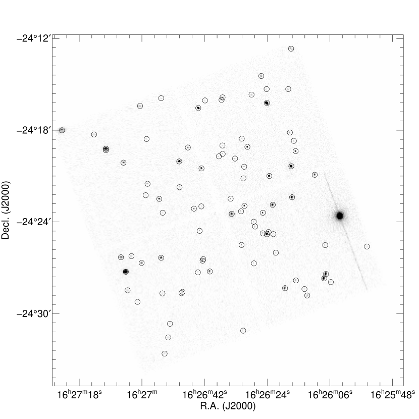
Figure 1:

Figure 2:

Figure 3:

Figure 4:

Figure 5:

Figure 6:

Figure 7:

Figure 8:

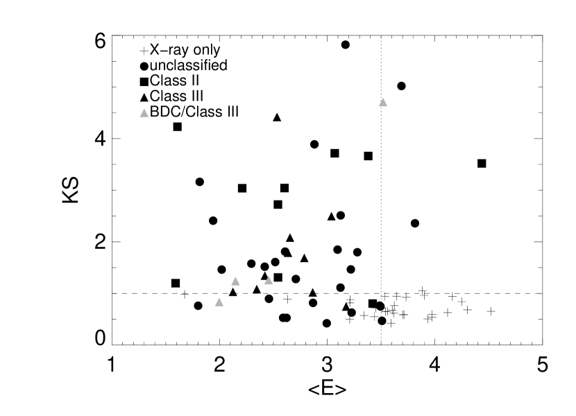
Figure 9a:

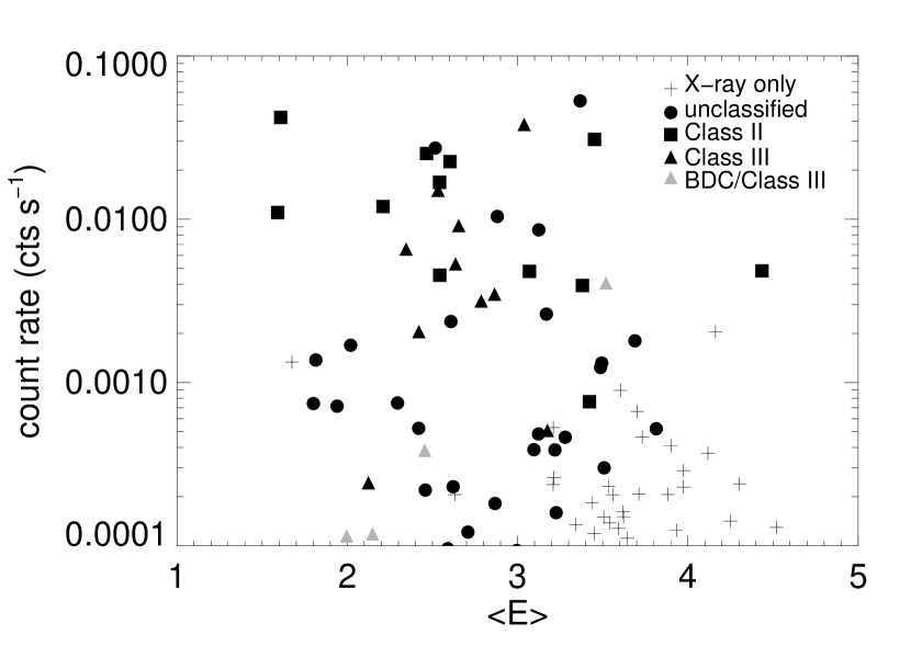
Figure 9b:

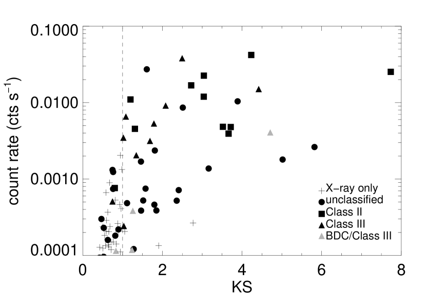
Figure 9c:

Figure 10:

Figure 11:

Figure 12:

Figure 13:

Figure 14:

Figure 15:

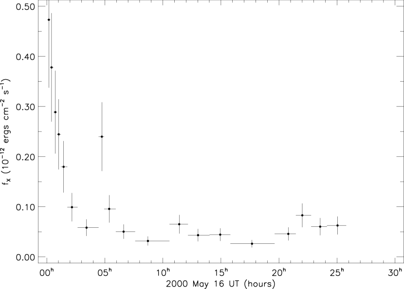
Figure 16:

Figure 17:

Figure 18:

References

- Anders & Grevesse (1989) Anders, E. & Grevesse, N. 1989, Geochim. Cosmochim. Acta, 53, 197
- André et al. (1992) André, P., Deeney, B.D., Phillips, R.B., & Lestrade, J.F., ApJ, 401, 667
- André et al. (1990) André, P., Martin-Pintado J., Despois, D., & Montmerle, T. 1990, A&A, 236, 180
- Allen et al. (2002) Allen, L.E., Myers, P.C., DiFrancesco, J., Mathieu, R., Chen, H., & Young, E. 2002, ApJ, 566, 993
- André et al. (1988) André, P., Montmerle, T., Feigelson, E.D., Stine, P.C., & Klein, K.-L. 1988, ApJ, 335, 940
- André et al. (1991) André, P., Phillips, R.B., Lestrade, J.-F., & Klein, K.-L. 1991, ApJ, 376, 630
- André & Montmerle (1994) André, P., & Montmerle, T. 1994, ApJ, 420, 837
- Armitage & Clarke (1996) Armitage, P.J., & Clarke, C.J. 1996, MNRAS, 280, 458
- Audard et al. (2001) Audard, M., Güdel, M., & Mewe, R. 2001, A&A, 365, L318
- Babel & Montmerle (1997a) Babel, J., & Montmerle, T. 1997a, A&A, 323, 121
- Babel & Montmerle (1997b) Babel, J., & Montmerle, T. 1997b, ApJ, 485, L29
- Babu & Feigelson (1996) Babu, G.J., & Feigelson, E.D. 1996, Astrostatistics (London: Chapman & Hall)
- Barsony et al. (1997) Barsony, M., Kenyon, S.J., Lada, E. A., & Teuben, P.J. 1997, ApJS, 112, 109
- Bessell & Brett (1988) Bessell, M.S. & Brett, J.M. 1988, PASP, 100, 1134
- Bieging, Cohen, & Schwartz (1984) Bieging, J.H., Cohen, M., & Schwartz, P.R. 1984, ApJ, 282, 699
- Bontemps et al. (2001) Bontemps, S., André, P., Kaas, A.A., Nordh, L., Olofsson, G., Huldtgren, M., Abergel, A., Blommaert, J., Boulanger, F., Burgdorf, M., Cesarsky, C.J., Cesarsky, D., Copet, E., Davies, J., Falgarone, E., Lagache, G., Montmerly, T., Pérault, M., Persi, P., Prusti, T., Puget, J.L., & Sibille, F. 2001, A&A, 372, 173 (ISO)
- Bouvier & Appenzeller (1992) Bouvier, J., & Appenzeller, I. 1992, A&AS, 92, 481
- Casanova et al. (1995) Casanova, S., Montmerle, T., Feigelson, E.D., & André, P. 1995, ApJ, 439, 752
- Castelaz et al. (1985) Castelaz, M.W., Hackwell, J.A., Grasdalen, G.L., Gehrz, R.D., & Gullixson, C. 1985, ApJ, 290, 261
- Chini (1981) Chini, R. 1981, A&A, 99, 346
- Ciliegi & Maccacaro (1997) Ciliegi, P., & Maccacaro, T. 1997, MNRAS, 292, 338
- Clarke et al. (1995) Clarke, C.J., Armitage, P.J., Smith, K.W., & Pringle, J.E. 1995, MNRAS, 273, 639
- Cowie et al. (2002) Cowie, L. L., Garmire, G. P., Bautz, M. W., Barger, A. J., Brandt, W. N., & Hornschemeier, A. E. 2002, ApJ, 566, L5
- Daniel et al. (2002) Daniel, K.J., Linsky, J.L., & Gagné, M. 2002, ApJ, 578, in press
- DolidZe & Arakelian (1959) Dolidze, M.V., & Arakelian, M.A. 1959, AZh, 36, 444 (DoAr)
- Doppmann, Jaffe, & White (2003) Doppmann, G.W., Jaffe, D.T., & White, R.J. 2003, AJ, 126, 3043
- Draine (1989) Draine, B.T. 1989, in Proceedings of the 22nd ESLAB Symposium on Intrared Spectroscipy in Astronomy, ed. B.H. Kaldeich, ESA SP-290, 93
- Duchene, Ghez, & McCabe (2001) Duchene, G., Ghez, A.M., & McCabe, C. 2001, BAAS, 33, 1435 (Abst. 89.06)
- Elias (1978) Elias, J. 1978, ApJ, 224, 453
- Feigelson et al. (2002) Feigelson, E.D., Broos, P., Gaffney III, J.A., Garmire, G., Hillenbrand, L.A., Pravdo, S.H., Townsley, L., & Tsuboi, Y. 2002, ApJ, 574, 278
- Feigelson et al. (2003) Feigelson, E.D., Gaffney, J.A., Garmire, G., Hillenbrand, L.A., & Townsley, L. 2003, ApJ, 584, 911
- Feigelson & Montmerle (1999) Feigelson, E.D., & Montmerle, T. 1999, ARA&A, 37, 363
- Feigelson et al. (1994) Feigelson, E.D., Welty, A.D., Imhoff, C.L., Hall, J.C., Etzel, P.B., Phillips, R.B., & Lonsdale, C.J. 1994, ApJ, 432, 373
- Flaccomio, Micela, & Sciortino (2003) Flaccomio, E., Micela, G., & Sciortino, S. 2003, astro-ph, 2329
- Flaccomio et al. (2003) Flaccomio, E., Damiani, F., Micela, G., Sciortino, S., Harnden, F. R., Murray, S. S., & Wolk, S. J. 2003, ApJ, 582, 398
- Flaccomio, Micela, & Sciortino (2003) Flaccomio, E., Micela, G., & Sciortino, S. 2003, A&A, 397, 611
- Gagné et al. (1995) Gagné, M., Caillault, J.-P., & Stauffer, J.R. 1995, ApJ, 445, 280
- Gagné et al. (1997) Gagné, M., Caillault, J.-P., Stauffer, J.R., & Linsky, J.L. 1997, ApJ, 478, L87
- Gagné et al. (2002) Gagné, M., Cohen, D., Owocki, S., & Ud-Doula, A. 2002, The High Energy Universe at Sharp Focus, ed. E.M. Schlegel& S.D. Vrtilek, ASP Conference Series (ASP: San Francisco), 262, 31
- Galli & Shu (1993) Galli, D., & Shu, F.H. 1993, ApJ, 417, 220
- Gehrels (1986) Gehrels, N. 1986, ApJ, 303, 336
- Ghez et al. (1995) Ghez, A.M., Weinberger, A.J., Neugebauer, G., Matthews, K., & McCarthy, D.W. 1995, AJ, 110, 753
- Grasdalen et al. (1973) Grasdalen, G. L., Strom, K. M., & Strom, S. E. 1973, ApJ, 184, L53 (GSS)
- Gómez et al. (2003) Gómez, M., Stark, D.P., Whitney, B.A., & Churchwell, E. 2003, AJ, 126, 863
- Greene & Lada (1997) Greene, T.P., & Lada, C.J. 1997, AJ, 114, 2157
- Greene & Meyer (1995) Greene, T.P., & Meyer, M.R. 1995, ApJ, 450, 233
- Greene & Young (1992) Greene, T.P., & Young, E.T. 1992, ApJ, 395, 516 (GY)
- Greene et al. (1994) Greene, T.P., Wilking, B.A., André, P., Young, E.T., & Lada, C.J. 1994, ApJ, 434 ,614
- Grosso (2001) Grosso, N. 2001, A&A, 370, L22
- Grosso et al. (1997) Grosso, N., Montmerle, T.,Feigelson, E., Andra, P., Casanove, S., & Gregorio-Hetem 1997, Nature, 387, 56
- Grosso et al. (2000) Grosso, N., Montmerle, T., Bontemps, S., André, P., & Feigelson, E.D. 2000, A&A, 359, 113
- Güdel, M. & Benz (1993) Güdel, M. & Benz, A. 1993, ApJ, 405, L63
- Güdel et al. (1999) Güdel, M., Linsky, J.L., Brown, A., & Nagase, F. 1999, ApJ, 511, 405
- Haisch et al. (1983) Haisch, B.M., Linsky, J.L., Bornmann, P.L., Stencel, R.E., Antiochos, S.K., Golub, L., & Vaiana, G.S. 1983, 267, 280
- Haisch et al. (2001) Haisch, K.E., Lada, E.A., Pina, R.K., Telesco, C.M., & Lada, C.L. 2001, AJ, 121, 1512
- Imanishi, Koyama, & Tsuboi (2001) Imanishi, K., Koyama, K., & Tsuboi, Y. 2001, ApJ, 557, 747
- Imanishi et al. (2002) Imanishi, K., Tsujimoto, M., & Koyama, K. 2002, ApJ, 572, 300
- Kamata et al. (1997) Kamata, Y., Koyama, K., Tsuboi, Y., & Yamauchi, S. 1997, PASJ, 49, 461
- Kastner et al. (2002) Kastner, J. H., Huenemoerder, D. P., Schulz, N. S., Canizares, C. R., & Weintraub, D. A. 2002, ApJ, 567, 434
- Knude & Hog (1998) Knude, J. & Hog, E. 1998, A&A, 338, 897
- Kopp & Poletto (1993) Kopp, R.A., & Poletto, G. 1993, ApJ, 418, 496
- Koyama et al. (1994) Koyama, K., Maeda, Y., Ozaki, M., Ueno, S., Kamata, Y., Tawara, Y., Skinner, S., & Yamauchi, S. 1994, PASJ, 46, L125
- Krishnamurthi et al. (2000) Krishnamurthi, A., Reynolds, C., Linsky, J., Martín, E., & Gagné M. 2001, AJ, 121, 337
- Lavalley et al. (1992) Lavalley, M., Isobe, T., & Feigelson, E. 1992, in Astronomical Data Analysis Software and Systems I, A.S.P. Conf. Series (vol. 25), eds. D. Worrall, C. Biemesderfer, & J. Barnes, 245
- Leous et al. (1991) Leous, J. A., Feigelson, E.D., André, P., & Montmerle, T. 1991, ApJ, 379, 683 (LFAM)
- Loren et al. (1990) Loren, R. B., Wootten, A., & Wilking, B. A. 1990, ApJ, 365, 269
- Luhman & Rieke (1999) Luhman, K.L., & Rieke, G.H. 1999, ApJ, 525,440
- Lynds (1962) Lynds, B.T. 1962, ApJS, 7, 1
- Maccacaro et al. (1988) Maccacaro, T., Gioga, I.M., Wolter, A., Zamorani, G., & Stocke, J.T. 1988, ApJ, 326, 680
- Martín et al. (1998) Martín, E.L., Montmerle, T., Gregorio-Hetem, J., & Casanova, S. 1998, MNRAS, 300, 733
- Meyer, Calvet, & Hillenbrand (1997) Meyer, M.R., Calvet, N., & Hillenbrand, L.A. 1997, AJ, 114, 288
- Mighell (1999) Mighell, K.J. 1999, ApJ, 518, 380
- Mokler & Stelzer (2002) Mokler, F. & Stelzer, B. 2002, A&A, 391, 1025
- Montmerle et al. (1983) Montmerle, T., Koch-Miramond, L., Falgarone, E., & Grindlay, J. 1983, ApJ, 269, 182
- Montmerle et al. (1991) Montmerle, T. 1991, in The Physics of Star Formation and Early Stellar Evolution, ed. C.J. Lada, & N.D. Kylafis (Dordrecht: Kluwer), 675
- Montmerle et al. (2000) Montmerle, T., Grosso, N., Tsuboi, Y., & Koyama, K. 2000, ApJ, 532, 1097
- Morrison & McCammon (1983) Morrison, R. & McCammon, D. 1983, ApJ, 270, 119
- Neuhäuser et al. (1999) Neuhäuser, R., Briceño, C., Comerón, F., Hearty, T., Martín, E.L., Schmitt, J.H.M.M., Stelzer, B., Supper, R., Voges, W., & Zinnecker, H. 1999, A&A, 343, 883
- Nousek & Shue (1989) Nousek, J.A. & Shue, D.R. 1989, ApJ, 342, 1207
- Owocki et al. (1988) Owocki, S.P., Castor, J.I., & Rybicki, G.B. 1988, ApJ, 335, 914
- Phillips et al. (1991) Phillips, R.B., Lonsdale, C.J., & Feigelson, E.D. 1991, ApJ, 382, 261
- Pontoppidan et al. (2002) Pontoppidan, K.M., Schöier, F.L., van Dishoeck, E.F., & Dartois, E. 2002, A&A, 393, 585
- Predehl & Schmitt (1995) Predehl, P., & Schmitt, J.H.M.M. 1995, A&A, 293, 889
- Preibisch & Zinnecker (2002) Preibisch, T. & Zinnecker, H. 2002, AJ, 123, 1613
- Press et al. (1992) Press, W.H., Teukolsky, S.A., Vetterling, W.T., & Flannery, B.P. 1992, Numerical Recipes in FORTRAN: The Art of Scientific Computing (2d ed., New York: Cambridge U. Press), 617
- Rebull et al. (2001) Rebull, L.M., Wolff, S.C., Strom, S.E., & Makidon, R.B. 2001, ApJ, in press
- Rieke & Lebofsky (1985) Rieke, G.H. & Lebofsky, M.J. 1985, ApJ, 288, 618
- Shu et al. (1994) Shu, F.H., et al. 1994, ApJ, 429, 781
- Simon et al. (1995) Simon, M., Ghez, A.M., Leinert, Ch., Cassar, L., Chen, W.P., Howell, R.R., Jameson, R.F., Matthews, K., Neugebauer, G., & Richichi, A. 1995, ApJ, 443, 625
- Skinner (1993) Skinner, S. 1993, ApJ, 408, 660
- Skinner, Walter & Yamauchi (1995) Skinner, S., Walter, F., & Yamauchi, S. 1995, in Rountgenstrahlung from the Universe, 69
- Skinner & Yamauchi (1996) Skinner, S., & Yamauchi, S.,1996, ApJ, 471, 987
- Smith, Brickhouse, Liedahl, & Raymond (2001) Smith, R. K., Brickhouse, N. S., Liedahl, D. A., & Raymond, J. C. 2001, ApJ, 556, L91
- Stassun et al. (2004) Stassun, K.G., Ardila, D.R., Barsony, M., Basri, G., & Mathieu, R.D. 2004, AJ, in press (astro-ph/0403159)
- Stelzer & Neuhäuser (2001) Stelzer, B., & Neuhäuser, R. 2001, A&A, 377, 538
- Stelzer et al. (2000) Stelzer, B., Neuhäuser, R., & Hambaryan V. 2000, A&A, 356, 949
- Stephens (1974) Stephens, M.A. 1974, J. Amer. Statistical Assoc., 69, 730
- Stine et al. (1988) Stine, P.C., Feigelson, E.D., André, P., & Montmerle, T., 1988, AJ, 96, 1394 (SFAM)
- Stocke et al. (1991) Stocke, J.T., Morris, S.L., Gioia, I.M., Maccacaro, T., Schild, R., Wolter, A., Fleming, T.A., & Henry, J.P. 1991, ApJS, 76, 813
- Strom et al. (1995) Strom, K.M., Kepner, J., & Strom, S.E. 1995, ApJ, 438, 813 (SKS)
- Townsley et al. (2000) Townsley, L.K., Broos, P.S., Garmire, G.P., Nousek, J.A. 2000, ApJ, 534, L139
- Tsuboi et al. (1998) Tsuboi, Y., Koyama, K., Murakami, H., Hayashi, M., Skinner, S., & Ueno, S. 1998, ApJ, 503, 894
- Tsuboi et al. (2000) Tsuboi, Y., Imanishi, K., Koyama, K., Grosso, N., & Montmerle, T. 2000, ApJ, 532, 1089
- Uchida & Shibata (1984) Uchida, Y., & Shibata, K. 1984, PASJ, 36, 105
- Vrba et al. (1975) Vrba, F.J., Strom, K.M., Strom, S.E., & Grasdalen, G.L. 1975, ApJ, 197, 77 (VSSG)
- Vuong et al. (2003) Vuong, M.H., Montmerle, T., Grosso, N., Feigelson, E.D., Verstraete, L., & Ozawa, H. 2003, A&A, 408, 581
- Weintraub et al. (1993) Weintraub, D.A., Kastner, J.H., Griffith, L.L., & Campins, H. 1993, AJ, 105, 271
- Weisskopf et al. (2002) Weisskopf, M.C., Brinkman, B., Canizares, C., Garmire, G., Murray, S., & Van Speybroeck, L.P. 2002, PASP, 114, 1
- Wilking et al. (1987) Wilking, B.A., Schwartz, R.D., & Blackwell, J.H., 1987, AJ, 94, 106
- Wilking et al. (1989) Wilking, B.A., Lada, C.J., & Young, E.T., 1989, ApJ, 340, 823
- Wilking et al. (1999) Wilking, B. A., Greene, T. P., & Meyer, M. R. 1999, AJ, 117, 469
- Wilking et al. (2001) Wilking, B. A., Bontemps, S., Schuler, R.E., Greene, T. P., & André, P. 2001, ApJ, 551, 357
- Wittet (1974) Wittet, D.C.B. 1974, MNRAS, 168, 371
- Zamorani et al. (1984) Zamorani, G., Giommi, P., Maccacaro, T., Tananbaum, H. 1984, ApJ, 278, 28
- Zhang, Wootten, & Ho (1997) Zhang, Q., Wootten, A., & Ho, P.T.P. 1997, ApJ, 475, 713