Dark matter in elliptical galaxies: I. Is the total mass density profile of the NFW form or even steeper?

Abstract

Elliptical galaxies are modelled as Sérsic luminosity distributions with density profiles (DPs) for the total mass adopted from the DPs of haloes within dissipationless $\Lambda$CDM N-body simulations. Ellipticals turn out to be inconsistent with cuspy low-concentration NFW models representing the total mass, nor are they consistent with a steeper $-1.5$ inner slope, nor with the shallower models proposed by Navarro et al. (2004), nor with NFW models 10 times more concentrated than predicted, as deduced from several X-ray observations: the mass models, extrapolated inwards, lead to local mass-to-light ratios that are smaller than the stellar value inside an effective radius ($R_{e}$), and to central aperture velocity dispersions that are much smaller than observed. This conclusion remains true as long as there is no sharp steepening (slope $<-2$) of the dark matter (DM) DPs just inside 0.01 virial radii.

The too low total mass and velocity dispersion produced within $R_{e}$ by an NFW-like total mass profile suggests that the stellar component should dominate the DM one out to at least $R_{e}$. It should then be difficult to kinematically constrain the inner slope of the dark matter DP of ellipticals. The high concentration parameters deduced from X-ray observations appear to be a consequence of fitting an NFW model to the total mass DP made up of a stellar component that dominates inside and a DM component that dominates outwards.

An appendix gives the virial mass dependence of the concentration parameter, central density, and total mass of the Navarro et al. model. In a 2nd appendix are given single integral expressions for the velocity dispersions averaged along the line-of-sight, in circular apertures and in thin slits, for general luminosity density and mass distributions, with isotropic orbits.

1 Introduction

There has been much recent progress on the photometric characterization of elliptical galaxies. Whereas a variety of models for the optical surface brightness profiles of ellipticals have been used in the past, such as the Hubble-Reynolds law (Reynolds, 1913), the analytical King (1962) or modified Hubble law, the projection of the isothermal spheres truncated in phase space (King, 1966) and the $R^{1/4}$ law (de Vaucouleurs, 1948), none provides an adequate fit to the surface photometry of the large majority of elliptical galaxies. However, there has been a recent consensus on the applicability to virtually all elliptical galaxies (Caon, Capaccioli, & D’Onofrio, 1993; Bertin, Ciotti, & Del Principe, 2002) of the generalization (hereafter, Sérsic law) of the $R^{1/4}$ law proposed by Sersic (1968), which can be written as

$$I(R)=I_{0}\exp\left[-\left({R\over a_{S}}\right)^{1/m}\right]\ ,$$ (1)

where $I$ is the surface brightness, $a_{S}$ the Sérsic scale parameter, and $m$ the Sérsic shape parameter, with $m=4$ recovering the $R^{1/4}$ law. Moreover, strong correlations have been reported between the shape parameter $m$ and either luminosity or effective (half projected light) radius $R_{e}$ (Caon et al., 1993, see also Prugniel & Simien, 1997, and references therein).

On the other hand, there is still much uncertainty on the importance of dark matter in elliptical galaxies, especially in their outer regions. Even in the spherical case considered in this paper, kinematical modelling of ellipticals usually cannot disentangle the degeneracy between the uncertainty of their gravitational potential and that of their internal kinematics (the anisotropy of their velocity ellipsoid), unless velocity profiles or at least 4th order velocity moments are considered (Merritt, 1987; Rix & White, 1992; van der Marel & Franx, 1993; Gerhard, 1993; Łokas & Mamon, 2003; Katgert et al., 2004).

Analyses of diffuse X-ray emission in elliptical galaxies have the advantage that the equation of hydrostatic equilibrium has no anisotropy term within it, so in spherical symmetry, one easily derives the total mass distribution through (e.g. Fabricant et al., 1980)

$$M(r)=-{k\,T(r)\,r\over G\mu m_{p}}\,\left({{\rm d}\ln n\over{\rm d}\ln r}+{{\rm d}\ln T\over{\rm d}\ln r}\right)\ ,$$ (2)

where $k$ is the Boltzmann constant, while $T$, $n$ and $\mu m_{p}$ are respectively the temperature, electron density and mean particle mass of the plasma. However, it is crucial to measure $T(r)$ and its gradient, and unfortunately, even with the two new generation X-ray telescopes XMM-Newton and Chandra, it is difficult to achieve such measurements beyond some fraction of 1/2 the virial radius for galaxy clusters (Arnaud et al., 2002; Pratt & Arnaud, 2002) but much less for elliptical galaxies. Moreover, the X-ray emission from elliptical galaxies is the combination of two components: diffuse hot gas swimming in the gravitational potential as well as direct emission from individual stars, and it can be highly difficult to disentangle the two (see Brown & Bregman, 2001).

On the theoretical front, cosmological simulations of large chunks of the Universe dominated by cold dark matter (CDM) have recently reached enough mass and spatial resolution that there appears to be a convergence on the structure and internal kinematics of the bound structures, usually referred to as haloes, in the simulations. In particular, the density profiles appear to converge to one with an outer slope of $\simeq-3$ and an inner slope between $-1$ (Navarro, Frenk, & White, 1995, 1996) and $-3/2$ (Fukushige & Makino, 1997; Moore et al., 1999; Ghigna et al., 2000), see also Power et al. (2003); Fukushige et al. (2004).

In this paper, we consider the general formula that Jing & Suto (2000) found to provide a good fit to simulated haloes:

$$\rho(r)\propto\left({r\over a_{h}}\right)^{-\alpha}\,\left[1+\left({r\over a_{h}}\right)\right]^{\alpha-3}\ ,$$ (3)

where $\alpha=1$ (hereafter ‘NFW’) or 3/2 (hereafter ‘JS–1.5’), and ‘$h$’ stands for halo. These profiles fit well the density profiles of cosmological simulations out to the virial radius $r_{v}$, wherein the mean density is $\Delta\approx 200$ times the critical density of the Universe. The ratio of virial radius to scale radius is called the concentration parameter:

$$c={r_{v}\over a_{h}}\ .$$ (4)

Very recently, a number of studies have proposed better analytic fits to the density (Navarro et al., 2004; Diemand et al., 2004) or circular velocity (Stoehr et al., 2002; Stoehr, 2005) profiles of simulated haloes. In particular, the formula of Navarro et al.

$${d\ln\rho\over d\ln r}=-2\,\left({r\over r_{-2}}\right)^{1/\mu}\ ,$$ (5)

where $\mu\simeq 6$ and $r_{-2}$ is the radius of slope $-2$, is attractive because it converges to a finite central density at very small scales and steepens progressively at outer radii to produce a finite mass. Moreover, Navarro et al. obtained their fits to the logarithmic slope of the density profile, while Diemand et al. fit to the density profile and Stoehr and collaborators to the circular velocity profile. Since the density and circular velocity respectively involve single and double integrals of the logarithmic slope profile, the latter two can mask subtle variations only picked up in the logarithmic slope. For these reasons, we shall add the Navarro et al. model in the present work.

In a previous paper (Łokas & Mamon, 2001, hereafter paper I), we showed that projected NFW density profiles could, in principle, be fit to Sérsic profiles with $m\simeq 3$. However, there are three reasons to disregard this match as a proof that mass follows light throughout elliptical galaxies:

1. As shown in Fig. 12 of paper I, projected NFW density profiles fit the Sérsic profiles only within a narrow range of Sérsic shape parameters $2.7\leq m\leq 4.0$, given reasonable NFW concentration parameters with ($5\leq c\leq 22$), whereas ellipticals are fit by Sérsic profiles in the much wider range: from $m=0.5-0.6$ for cluster dwarf ellipticals (Caon et al., 1993; Binggeli & Jerjen, 1998; Márquez et al., 2000) to $m=16$ (Caon et al.) or 8 (Graham, 1998), 7 (D’Onofrio, 2001) or at least 5.6 (Márquez et al., 2000).

2. The fits produced enormous effective radii, much larger than observed.

3. The fits produced $m$ increasing with concentration parameter $c$ (again Fig. 12 of paper I — which plots $1/m$ versus $c$). But, $c$ is known to decrease with mass within the virial radius (Navarro, Frenk, & White, 1997; Jing & Suto, 2000), while $m$ is known to increase with luminosity (Caon et al.; Prugniel & Simien, 1997, see Fig. 1 below). Hence, one arrives at the very unlikely result that galaxy luminosity decreases with increasing mass within the virial radius.

The conclusions of paper I have been confirmed in a recent analysis of Merritt et al. (2005), who have recently shown that the halos in dissipationless cosmological $N$-body simulations are also well fit in projection by a Sérsic model with $m\simeq 3$. This is not surprising since the NFW model provides an adequate fit to the density profiles of halos in dissipationless cosmological simulations. But, in contrast to the case of the divergent-mass NFW models, point 2 should not be relevant for convergent-mass halos described by the Sérsic or Navarro et al. models. Nevertheless, the relevance of points 1 and 3 remain relative to the work of Merritt et al..

Now there are several strong indications that mass does not follow light in elliptical galaxies: first, from the kinematics of neutral gas (Bertola et al., 1993), and second from X-rays (eq. [2]), albeit with the simplifying and probably optimistic assumption of isothermality. Some studies point to $M/L_{\rm opt}$ increasing outwards, such as Jones et al. (1997) for NGC 1399. Also, Buote et al. (2002) use the variation of the ellipticity of the X-ray isophotes to conclude that mass does not follow light in an elongated elliptical galaxy (NGC 720).

Recent analyses of X-ray data by Sato et al. (2000), Wu & Xue (2000), and Lloyd-Davies & Ponman (2002) (quoted in Lloyd-Davies et al., 2002) conclude (using eq. [2]) that the total mass of ellipticals, groups and clusters are indeed well fit by an NFW model, but with typically ten times larger concentration than measured in cosmological simulations for the mass range of elliptical galaxies. Surprisingly, there have been no detailed studies of these high concentration total density profiles arising from the X-ray observations.

Whereas the NFW profile was first established with cosmological simulations including a dissipative gaseous component (Navarro et al., 1995), most confirmations of the NFW or JS–1.5 profiles have come from simulations without gas, which can achieve a much greater mass resolution. Hence, one may ask if the density profiles of haloes found in cosmological $N$-body simulations of cold dark matter in a flat universe with $\Omega_{\Lambda}\simeq 0.7$ (globally referred hereafter as $\Lambda$CDM) represent the total density of observed cosmic structures or only their dark matter component. Given that the average baryon fraction in the Universe is small, one could think that when structures such as elliptical galaxies form by collapse, the baryons simply follow the dark matter without affecting it, and the total mass profile would resemble the low concentration cuspy models found in the cosmological simulations. Alternatively, since gas dynamics is dissipative, there may be a density threshold beyond which the gas will decouple from the dark matter, and then the central regions of ellipticals would be dominated by gas and later stars that form from it. The low-concentration cuspy density profiles found in the cosmological simulations would then only apply to the dark matter. Moreover, if the baryons dominate the dark matter at small radii, the dark matter will re-adjust itself within the gravitational potential dominated by the baryons (in a process often referred to as adiabatic contraction, see, e.g., Gnedin et al., 2004), so that even the dark matter density profile may differ substantially from the predictions of the dissipationless $\Lambda$CDM simulations. Also, if ellipticals form by major mergers of spirals (Toomre, 1977; Mamon, 1992), the distribution of baryons (mainly stars) will be set by violent relaxation operating during the merger, and if the baryonic fraction is low in the outer regions of the two merging spirals, the merger remnant should also show a lower baryon fraction in the outer regions.

In the present paper, we abandon the hypothesis of paper I of constant mass-to-light ratio, and we consider the next simplest approach, asking ourselves whether the radial profiles of density coming out of dissipationless cosmological $N$-body simulations are consistent with the observations (surface photometry and spectroscopy) of elliptical galaxies, for the total mass (Sec. 3), and whether low or high concentration parameters are required. We will not consider here the response of the dark matter component to the dissipative baryonic component (e.g., the adiabatic contraction of the dark matter).

We begin, in Sec. 2, with a summary of the luminosity and mass models of elliptical galaxies that we adopt in this paper. In a companion paper (Mamon & Łokas, 2005), we go one step further and confront the general observed trends in elliptical galaxies with the predictions from a 4-component model of ellipticals with stars, dark matter, hot gas and a central black hole, allowing for slight radial velocity anisotropy, as seen in cosmological $N$-body simulations.

2 Basic equations

2.1 Distribution of optical light

The Sérsic (eq. [1]) optical surface brightness profile that represents the projected stellar distribution, can be deprojected according to the approximation first proposed by Prugniel & Simien (1997)

$$\ell(r) = \ell_{1}\,\widetilde{\ell}(r/a_{S})$$ (6)

$$\widetilde{\ell}(x) \simeq x^{-p}\,\exp\left(-x^{1/m}\right)\ ,$$ (7)

$$\ell_{1} = \left\{{\Gamma(2m)\over\Gamma[(3-p)\,m]}\right\}\,{I_{0}\over 2\,a_{S}}\ ,$$ (8)

$$p \simeq 1.0-0.6097/m+0.05463/m^{2}\ ,$$ (9)

where $\Gamma(a)$ is the gamma function. The last equation is from Lima Neto et al. (1999) who argue that equations (6) and (7) then provide a better deprojection of the Sérsic profile (eq. [1]), and in a wider range of $m$ (good to better than 5% accuracy for $0.55<m<10$ within $0.01<R/R_{e}<1000$, where over 99.5% of the light lies) than a previous approximation of $p(m)$ proposed by Prugniel & Simien.

The integrated luminosity corresponding to equations (6), (7) and (8) is then (Lima Neto et al.)

$$L_{3}(r) = L\,\widetilde{L}_{3}(r/a_{S})$$ (10)

$$\widetilde{L}_{3}(x) = {\gamma\left[(3-p)m,x^{1/m}\right]\over\Gamma[(3-p)m]}\ ,$$ (11)

where $\gamma(a,x)$ is the incomplete gamma function and where the total luminosity of the galaxy is

$$L=2\pi m\,\Gamma(2m)\,I_{0}\,a_{S}^{2}=4\pi m\,\Gamma\left[(3-p)\,m\right]\,\ell_{1}\,a_{S}^{3}\ ,$$ (12)

as obtained by Young & Currie (1994) from the Sérsic surface brightness profile of equation (1), and which matches exactly the total luminosity obtained by integration of Lima Neto et al.’s approximate deprojected profile.

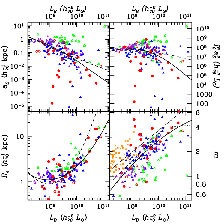
Figure 1: Correlations of Sérsic parameters of elliptical and S0 galaxies. Ellipticals in the Coma and Abell 496 clusters (filled triangles) and Abell 85 (empty triangles) measured by Marquez et al. (2000); ellipticals (filled circles) and S0s (open circles) in the Virgo and Fornax clusters measured by D’Onofrio (2001, restricted to the good-fitting cases, i.e. where $Q<3$ and $\chi_{r}^{2}<1.5$) and dwarf ellipticals in the Virgo cluster (crosses) and in the $m$ vs. $L$ plot measured by Binggeli & Jerjen (1998). These symbols are plotted in blue, purple, green, red, and orange in the electronic version of the Journal. The solid curves are the adopted fits, performed on $\log R_{e}$ vs. $\log L$ (eq. [16]) and $\log m$ vs. $\log L$ (eq. [17]), and used to estimate $a_{S}$ (eq. [18]) and $I_{0}\,a_{S}^{2}$ (eq. [12]), while the dashed curves represent the direct fits of $\log a_{S}$ vs. $\log L$ and $\log I_{0}\,a_{S}^{2}$ vs. $\log L$ and the corresponding relation for $R_{e}$ vs. $L$ (from eqs. [14] and [15]). The fits use the data of Márquez et al. omitting their Abell 85 values, combined with the data of D’Onofrio. The dotted broken line in the $m$ vs. $L$ plot is the mean relation from Prugniel & Simien (1997), while the dashed-dotted line is from Graham & Guzman (2003). The luminosities of the D’Onofrio galaxies are $H_{0}$-independent (see text).

Fig. 1 shows how the Sérsic parameters are correlated. The data are taken from

1. Binggeli & Jerjen (1998), who computed Sérsic parameters from fitting the cumulative luminosity profile for dwarf ellipticals in Virgo.

2. Márquez et al. (2000), who did the same for normal ellipticals in the Coma, Abell 85 and Abell 496 clusters. We converted their angular sizes to distances, by simply assigning Hubble distances to each cluster, assuming no peculiar motion relative to us. We also converted their $V$-magnitudes to $B$-band luminosities, assuming $B-V=0.96$ (typical of elliptical galaxies, e.g. Fukugita et al., 1995) and (e.g. Colina et al., 1996)

   $$M_{B}^{\odot}=5.45\ .$$ (13)

3. D’Onofrio (2001), who performed 2D fits of Sérsic + exponential models for galaxies in the Virgo and Fornax clusters. We corrected their luminosities by replacing their unique distance modulus by the surface brightness fluctuation (SBF) distance modulus of Tonry et al. (2001) when available, or otherwise by adding the median difference (0.18) between the SBF distance moduli and the unique value adopted by D’Onofrio for their 23 galaxies in common.

In principle, the 2D fitting method of D’Onofrio should be the most reliable, but for given clusters, the means trends in the data of Márquez et al. show much less scatter for individual clusters. Interestingly, the mean trends for Coma and Abell 496 agree well with the mean trend for the ellipticals and lenticulars of D’Onofrio, while the galaxies in the cluster Abell 85 (open triangles in Fig. 1) are systematically offset from the galaxies of the other two clusters, in such a manner that its distance, as simply derived from its redshift, appears 80% too large (as is clear from the correlations of $m$ vs. $L$, and consistent with the correlations in the other plots of Fig. 1), but it is highly improbable that the distance to Abell 85 is overestimated by such a large factor. Also, the dwarf ellipticals analysed by Binggeli & Jerjen (1998) appear to have a shape-luminosity relation that disagrees with those of Márquez et al. and D’Onofrio.

Discarding the Abell 85 data as well as the dwarf ellipticals of Binggeli & Jerjen (1998), one is left (circles and filled triangles) with fairly strong correlations in Fig. 1, where, in particular, the shape parameter $m$ correlates with luminosity (Caon et al., 1993).

For simplicity, we assume that elliptical galaxies constitute a one-parameter family, based on luminosity (or equivalently, on Sérsic shape $m$). Whereas such a one-parameter model of ellipticals is consistent with the Faber-Jackson (1976) relation between central velocity dispersion and luminosity, it is obviously an oversimplification, in view of the fundamental plane of elliptical galaxies, where the central velocity dispersion is a function of both luminosity and surface brightness (Dressler et al., 1987; Djorgovski & Davis, 1987).

We fit the parameter correlations of Fig. 1 with 2nd-order polynomials in log space (with iterative 3-$\sigma$ rejection of outliers), using the galaxies in Coma and Abell 496 of Márquez et al. (filled triangles in Fig. 1) and the ellipticals and S0s in Virgo of D’Onofrio (circles in Fig. 1). Now $a_{S}$ and $R_{e}$ are directly related through $m$ via

$$R_{e} = b^{m}\,a_{S}$$ (14)

$$b \simeq 2\,m-1/3+0.009876/m\ ,$$ (15)

where the latter relation is from Prugniel & Simien (1997). Similarly, $L$ and $I_{0}\,a_{S}^{2}$ are directly related through $m$ (eq. [12]). Therefore, we choose to obtain $a_{S}$ and $I_{0}\,a_{S}^{2}$ through the fits of $R_{e}$ vs. $L$, and $m$ vs. $L$:

$$\log h_{70}\,R_{e}^{\rm(fit)} \!\!\!\!=\!\!\!\! 0.34+0.54\,\log L_{10}+0.25\,\left(\log L_{10}\right)^{2}\ ,$$ (16)

$$\log m^{\rm(fit)} \!\!\!\!=\!\!\!\! 0.43+0.26\,\log L_{10}-0.044\,\left(\log L_{10}\right)^{2}\,,$$ (17)

where $L_{10}=h_{70}^{2}\,L_{B}/\left(10^{10}{\rm L_{\odot}}\right)$, $R_{e}^{\rm(fit)}$ is measured in kpc, and with $H_{0}=100\,h=70\,h_{70}\,\rm km\,s^{-1}\,Mpc^{-1}$. Then equations (14) and (15) lead to

$$a_{S}\simeq\left[b\left(m^{\rm(fit)}\right)\right]^{-m^{\rm(fit)}}R_{e}^{\rm(fit)}\ .$$ (18)

The fits of equations (16), (17) and the corresponding relation for $a_{S}$ from equation (18) are shown as solid curves in Fig. 1, whereas the dashed curves show the direct fits to $L$ for $a_{S}$ and $I_{0}\,a_{S}^{2}$. For example, for $L_{B}=10^{10}h_{70}^{-2}{\rm L_{\odot}}$, one has $m^{\rm(fit)}=2.7$, slightly lower than the value of $m=3.29$ inferred from the relation of Prugniel & Simien (1997). The fits can be considered to be uncertain to a factor 2 in $R_{e}$ and 1.5 in $m$ and we will propagate these uncertainties later in our analysis. Note that equation (16) produces effective radii that increase at decreasing luminosity for low $L$, which may not be very realistic. Similarly, equation (17) produces abnormally low values of $m$ at low luminosity, as the $m$ vs $L$ relation should flatten out at low luminosities to accommodate the dwarfs of Binggeli & Jerjen and because values of $m<1$ are rarely mentioned in the literature if at all. However, inspection of Fig. 1 indicates that equations (16) and (17) are both reasonably accurate for $L_{B}>2\times 10^{9}h_{70}^{-2}{\rm L_{\odot}}$.

2.2 Scalings of global properties

We adopt a fiducial luminosity of $L_{B}=L_{B}^{*}$ (the luminosity at the break of the field galaxy luminosity function). Liske et al. (2003) have compiled various measurements of the corresponding absolute magnitude $M^{*}$ and converted to their $B_{\rm MGC}$ band. Their median value is $M_{\rm MGC}^{*}=-19.6+5\,\log\,h=-20.37$ (for $h=0.7$), which is within 0.01 magnitude of their conversion of the 2dFGRS value of Norberg et al. (2002). Liske et al. give the transformation from the $B_{\rm MGC}$ system to the Landolt $B$ system: $B_{\rm MGC}=B-0.145\,(B-V)$. Given that elliptical galaxies have $B-V\simeq 0.96$ (Fukugita et al., 1995), we derive $M_{B}^{*}=-20.24$, which corresponds to $L_{B}^{*}=1.88\times 10^{10}\rm L_{\odot}$, again using $M_{B}^{\odot}=5.45$ (eq. [13]).

Given the mean luminosity density of the Universe $j$, and the mean mass density of the Universe $\Omega_{m}\,\rho_{\rm crit}$, the mean mass-to-light ratio of the Universe is

$$\overline{\Upsilon}=\Omega_{m}\,\Upsilon_{\rm closure}={3\,\Omega_{m}H_{0}^{2}\over 8\pi\,G\,j}\ .$$ (19)

Converting Liske et al.’s $j_{b_{J}}=1.99\times 10^{8}h\,\rm L_{\odot}\,Mpc^{-3}$ to the $B$ band with $B-b_{J}=0.28\,(B-V)$, initially proposed by Blair & Gilmore (1982) and inferred from both Liske et al. and Blanton et al. (2003), now assuming $\langle B-V\rangle=0.94$ (Norberg et al., 2002), with $M_{b_{J}}^{\odot}=5.3$ (Liske et al.), and converting the Hubble constant, we derive $j_{B}/(10^{8}\,h_{70}\,{\rm L_{\odot}}\,\rm Mpc^{-3})=1.25$. Similarly, Blanton et al. (2003) give blue band luminosity densities of $-14.98-2.5\,\log h$ and $-15.17-2.5\,\log h$ magnitude per Mpc³, when k-corrected to $z=0$ and $z=0.1$, respectively. For the local Universe ($z=0$), this translates to $j_{B}=1.04\times 10^{8}\,h_{70}\,{\rm L_{\odot}}\,\rm Mpc^{-3}$, again using equation (13). Since Liske et al. do not k-correct to $z=0$ and since the median redshift of the 2dFGRS is close to 0.1, we adopt a mean k-correction similar to the one found by Blanton et al.: $-14.98+15.17=0.19$ mag. This then leads to a 2dFGRS luminosity density, transformed to the $B$ band and k-corrected to $z=0$ of $j_{B}=1.05\times 10^{8}\,h_{70}\,{\rm L_{\odot}}\,\rm Mpc^{-3}$, in remarkable agreement with the SDSS value of Blanton et al.. Taking the mean of these 2dFGRS and SDSS luminosity densities, we derive a local closure mass-to-light ratio of $\Upsilon_{\rm closure}^{B}/h_{70}=1300$ and, with $\Omega_{m}=0.3$, we obtain

$$\overline{\Upsilon}_{B}=390\,h_{70}\ .$$ (20)

So for $L_{B}=L_{B}^{*}=1.88\times 10^{10}\,h_{70}^{-2}\,{\rm L_{\odot}}$, an unbiased universe would yield a total mass within the virial radius $\log h_{70}\,M_{t}=12.87$.

Two recent statistical analyses of galaxy properties suggest that $M/L_{B}$ has a non-monotonous variation with mass (or luminosity), with a minimum value around 100 for luminosities around $10^{10}\,{\rm L_{\odot}}$ (Marinoni & Hudson, 2002; Yang et al., 2003). Theoretical predictions by Kauffmann et al. (1999), based upon semi-analytical modelling of galaxy formation on top of cosmological $N$-body simulations also find a minimum of $\Upsilon_{B}/\overline{\Upsilon}_{B}=0.19$ at a similar luminosity, which translates to $\Upsilon_{B}=74\,h_{70}$ with equation (20). On the other hand, the internal kinematics of galaxy clusters are consistent with the mass-to-light ratio of the Universe given by equation (20): e.g. Łokas & Mamon (2003) derive $\Upsilon_{B}=351\,h_{70}$ for the Coma cluster.

In the following section, we will compare our mass-to-light ratios to those expected for old stellar populations. For example, Trujillo, Burkert, & Bell (2004) report a stellar mass-to-blue-light ratio $\Upsilon_{*,B}=7.1$ from an analysis of SDSS galaxies using the PEGASE (Fioc & Rocca-Volmerange, 1997) stellar population synthesis code and a Salpeter (1955) initial mass function (IMF). However, using different stellar population synthesis codes and several choices for the IMF, Gerhard et al. (2001) find values differing by a factor of 2 for given galaxies (e.g., $\Upsilon_{*,B}=4.2$ to 8.8 for the nearby elliptical, NGC 3379). We performed our own tests of the expected values of $\Upsilon_{*,B}$ given the extinction-corrected colours of nearby elliptical galaxies, with PEGASE, GALEXV (Bruzual & Charlot, 2003) and G. Worthey’s on-line model. We found a very large variety of stellar mass-to-light ratios for given colours, spanning from $\Upsilon_{*,B}=2$ to 12, depending on the IMF, its low- and high-mass cutoffs, the metallicity and the stellar evolution code. In particular, Salpeter’s IMF produces high values (as also found by Gerhard et al.), and GALEXV produces lower values for a given IMF in comparison with PEGASE. In the end, we adopt best values of $\Upsilon_{*,B}=8$ and 5, and a possible range of a factor 1.5 around the geometric mean ($\Upsilon_{*,B}=6.3$).

We also make use of the Faber-Jackson (1976) relation. We have compared the calibrations of de Vaucouleurs & Olson (1982), Bender et al. (1996), Kormendy et al. (1997, who make use of data from McElroy, 1995) and Forbes & Ponman (1999, who make use of data from Prugniel & Simien, 1996). Converting to the same value of $H_{0}$, we find that the correlation between the velocity dispersions averaged in circular apertures, $\sigma_{\rm ap}$ and the blue-band luminosities of Bender et al. are consistent with the analogous correlations of de Vaucouleurs & Olson, Kormendy et al. and Forbes & Ponman, but with less scatter, and extends to a large enough range of luminosities, with the following mean trend

$$\sigma_{\rm ap}=171\,{\rm km\,s}^{-1}\,\left({h_{70}^{2}\,L_{B}\over 10^{10}\,{\rm L_{\odot}}}\right)^{1/3.25}\ .$$ (21)

2.3 Distribution of total mass

We consider here 3 models for the total mass distribution: 1) the NFW model with inner slope $-1$; 2) a generalization of the NFW model introduced by Jing & Suto (2000) with inner slope $-3/2$ (JS–1.5, which is slightly different from the formula proposed by Moore et al., 1999); and 3) the convergent model of Navarro et al. (2004, hereafter Nav04, see eq. [5]). The total matter density profile can generally be written:

$$\rho(r) \!\!\!\!=\!\!\!\! {c^{3}\over g(c)}\,\left({M_{v}\over 4\pi\,r_{v}^{3}}\right)\,\widetilde{\rho}(r/a_{h})\ ,$$ (22)

$$\widetilde{\rho}(y) \!\!\!\!=\!\!\!\! \left\{\!\!\begin{array}[]{lll}y^{-\alpha}\,(1+y)^{\alpha-3}&\hbox{(NFW, JS--1.5)}\ ,\\ &\\ \exp\left(-{2\mu}\,y^{1/\mu}\right)&\hbox{(Nav04)}\ ,\end{array}\right.$$ (26)

$$g(y) \!\!\!\!=\!\!\!\! \left\{\!\!\!\!\begin{array}[]{ll}\ln(y+1)-y/(y+1)&\!\!\!\!\hbox{(NFW)}\ ,\\ &\\ 2\,\left[\sinh^{-1}\sqrt{y}-\sqrt{y/(y\!+\!1)}\right]&\!\!\!\!\hbox{(JS--1.5)}\ ,\\ &\\ {1\over 2}\,\left(2\,\mu\right)^{1-3\,\mu}\,\gamma\left[{3\,\mu},{2\,\mu}\,y^{1/\mu}\right]&\!\!\!\!\hbox{(Nav04)}\ ,\end{array}\right.$$ (32)

where $-\alpha$ is the inner slope, $c$ is the concentration parameter (eq. [4]), $a_{h}$ is the radius where the logarithmic slope is equal to $-2$ (NFW, Nav04) or $-9/4$ (JS–1.5, for which $a_{h}/2$ is the radius where the slope is $-2$), $\mu\simeq 6$ (appendix A), and $\sinh^{-1}x=\ln(x+\sqrt{x^{2}+1})$ for $x>0$. In equation (22), $M_{v}$ is the mass within the virial radius, defined such that the mean total density within it is $\Delta=200$ times the critical density of the Universe, $\rho_{\rm crit}=3\,H_{0}^{2}/(8\,\pi G)$, yielding a virial radius (see Navarro et al., 1997)

$$r_{v} = \left({2\,G\,M_{v}\over\Delta\,H_{0}^{2}}\right)^{1/3}\ ,$$ (33)

$$= 163\,h^{-1}\,{\rm kpc}\,\left({h\,M_{v}\over 10^{12}\,{\rm M_{\odot}}}\right)^{1/3}\ ,$$

$$= 206\,h_{70}^{-1}\,{\rm kpc}\,\left({h_{70}M_{v}\over 10^{12}\,{\rm M_{\odot}}}\right)^{1/3}\ ,$$

for $\Delta=200$. Equation (32) is derived by integrating equation (22) using equation (26), thus using equation (40) for the Nav04 model. Jing & Suto (2000) measured the concentration parameter $c$ (eq. [4]) from their $\Lambda$CDM (with cosmological density parameter $\Omega_{m}=0.3$ and dimensionless cosmological constant $\Omega_{\Lambda}=0.7$) simulations, which can be fit by the relations

$$c\simeq\left\{\begin{array}[]{ll}\displaystyle 10.2\,M_{12}^{-0.08}&(\hbox{NFW})\ ,\\ &\\ \displaystyle 4.9\,M_{12}^{-0.13}&(\hbox{JS--1.5})\ ,\end{array}\right.$$ (34)

where $M_{12}={hM_{v}/10^{12}{\rm M_{\odot}}}$. In Appendix A, we derive (eq. [44]) the concentration parameter for the Nav04 model:

$$c=8.1\,M_{12}^{-0.11-0.015\,\log M_{12}}\,$$

which is similar to the concentration parameters in equations (34).

X-ray data analyses (Sato et al., 2000; Wu & Xue, 2000; Lloyd-Davies & Ponman, 2002) based upon equation (2) conclude that the total mass of ellipticals, groups and clusters are indeed well fit by an NFW model, but their concentration parameters increase much faster for decreasing masses. Sato et al. give

$$c=73\,M_{12}^{-0.44}\ ,$$ (35)

while for the other two studies, the concentration parameter extrapolated to $M_{v}=10^{12}\,h^{-1}{\rm M_{\odot}}$ ($M_{12}=1$) is slightly over 100 and the slope is $-0.51$ in both cases. Note that Jing & Suto, Sato et al., and Lloyd-Davies & Ponman all define their virial quantities at the radius where the mean density is 200 times the critical value, while Wu & Xue define their virial radius where the mean density is 100 times the critical value, in accordance with the spherical top hat infall model for $\Omega_{m}=0.3,\Omega_{\Lambda}=0.7$. Interestingly, in their cosmological $N$-body simulations, Bullock et al. (2001) confirm high concentration parameters for the mass distribution within subhaloes of haloes (which may correspond to elliptical galaxies within clusters), with a steeper dependence of concentration on mass: $d\ln c/d\ln M\approx-0.3$.

The cumulative mass of the dark models used here can all be written

$$M(r) = M_{v}\,\widetilde{M}(r/a_{h})\ ,$$ (36)

$$\widetilde{M}(y) = {g(y)\over g(c)}\ ,$$ (37)

where $g$ is given in equation (32).

3 Results

3.1 Local mass-to-light ratios

The simplest check that cuspy $\Lambda$CDM models represent the total mass distribution of elliptical galaxies, i.e. the gravitational potential, is by checking that the mass at all radii is greater than the known contribution from stars.

Given equations (4), (6), (7), (8), (22), (26), and (32), the local mass-to-light ratio is

$$\Upsilon(r) = {\rho(r)\over\ell(r)}={\rho_{1}\over\ell_{1}}\,{\widetilde{\rho}(r/a_{h})\over\widetilde{\ell}(r/a_{S})}\ ,$$ (38)

$$= {m\,\Gamma[(3-p)m]\over g(c)}\,{M_{v}\over L}\,\eta^{3-\alpha}$$

$$\times\,x^{p-\alpha}\,(1+\eta x)^{\alpha-3}\exp\left(x^{1/m}\right)\ ,$$

where the second equality is restricted to the NFW and JS–1.5 models, with $x=r/a_{S}$, $\eta=a_{S}/a_{h}$, and $\alpha=1$ (NFW) or 3/2 (JS–1.5).

Fig. 2 shows the local $M/L$ profile for the Sérsic model with luminosity $L_{B}=L_{*}=1.88\times 10^{10}\,h_{70}^{-2}\,{\rm L_{\odot}}$ and our three adopted mass models with masses within the virial radius of $\log h_{70}^{-1}\,M_{v}=11.87$, 12.87, and 13.87, i.e. for mass-to-light ratios 0.1, 1, and 10 times the universal value (eq. [20]). The shaded region in Fig. 2 indicates the mass-to-light ratios inferred from stellar population synthesis (see Sec. 2.2), in the range where the surface brightness profile is well known (and where the Sérsic deprojection is considered accurate, see Sec. 2.1).

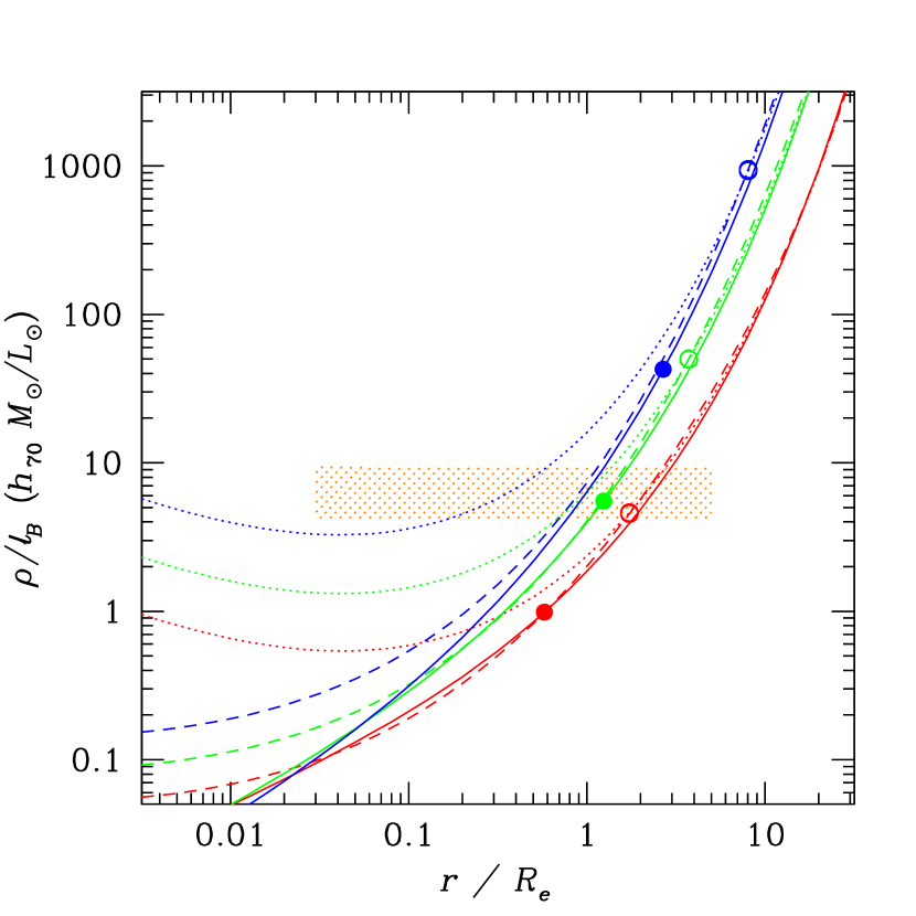
Figure 2: Local mass-to-light ratio profiles for the Sérsic distribution of luminosity $L_{B}=L_{B}^{*}=1.88\times 10^{10}\,h_{70}^{-2}\,{\rm L_{\odot}}$, with $m=3.1$ (eq. [17]) and $R_{e}=3.2\,h_{70}^{-1}\,\rm kpc$ (eq. [16]), and NFW (dashed curves), JS–1.5 (dotted curves), and Nav04 (solid curves) total mass distributions with $\log h_{70}^{-1}\,M_{v}=11.87$, 12.87, and 13.87 (mass-to-light ratios $\Upsilon_{B}=39,390,3900$, i.e. 0.1, 1, and 10 times the universal value of eq. [20]), increasing upwards (red, green, and blue in the electronic version of the Journal). The open circles represent $0.03\,r_{v}$, the minimum radius where the NFW and JS–1.5 models are accurate in representing the density profiles in structures found in cosmological $N$-body simulations, while the filled circles represent $0.01\,r_{v}$, which is the analogous radius for the Nav04 model. The curves are obtained with equation (38) using equations (4), (9), (14), (15), (16), (32), (33), and (34). The shaded region (orange in the electronic version of the journal) shows the mass-to-light ratio of the stellar populations of elliptical galaxies (in the range of radii where the Sérsic fits to the surface brightness profile are believed to be good, see Sec. 2.2).

Fig. 2 indicates that, at the lower limit of its spatial resolution ($0.01\,r_{v}\simeq 0.6\,R_{e}$), the low mass ($\Upsilon_{B}=39$) Nav04 model produces a lower mass-to-light ratio than stellar, reaching values as low as unity, inconsistent with all estimates of the stellar mass-to-light ratios of old (and red, as observed) stellar populations.

For the models with higher virial cumulative mass-to-light ratio, the local mass-to-light ratios are consistent with the expected stellar mass-to-light ratios in the range where these dark matter models are measured. However, simple inwards extrapolations of these mass models rapidly lead to sub-stellar mass-to-light ratios. For example, for the universal virial mass-to-light ratio ($\Upsilon_{B}=390$), the Nav04 model is consistent with the stellar mass-to-light ratio at the limit of its resolution, $r=0.01\,r_{v}\simeq 1.4\,R_{e}$. But if one wishes to ensure that the local mass-to-light ratio at lower radii remains higher than the stellar value, one then requires the mass model to have a density slope equal to that of a Sérsic model. From equations (6), (7) and (9), the slope of the deprojected Sérsic profile is $-p-b/m(r/R_{e})^{1/m}$. For $m=3.1$, one gets a slope of $-2.9$ at $1.4\,R_{e}$, and of $-1.4$ at $0.03\,R_{e}$. In comparison, for elliptical galaxies with $hM=10^{12}M_{\odot}$, for which the Nav04 resolution limit is $r=0.01\,r_{v}=1.4\,R_{e}=0.08\,r_{-2}$ (eq. [44]), then according to equation (5), the Nav04 model has a slope of $-1.3$, as also inferred from fig. 3 of Navarro et al.. While the density profile of the Nav04 model becomes shallower with decreasing radius (as do the density profiles of the NFW and JS–1.5 models), one must, on the contrary, assume that the profile suddenly steepens at $r<R_{e}$. The same argument applies for the NFW model. Hence, the NFW and Nav04 models cannot represent the total mass.

The cuspier nature of the JS–1.5 model makes it less sensitive to this criterion. Nevertheless, Fig. 2 indicates that a slope steeper than $-1.5$ is required to keep the mass-to-light ratio above the stellar value. Therefore, unless there is a sharp break in the density profiles inside the resolution radius to a slope that is considerably steeper than $-3/2$, any reasonable extrapolation of the mass-to-light ratio curves will lead to values lower than stellar.

Do the high-concentration NFW models found by Sato et al. (2000) for the total matter distribution also produce abnormally low mass-to-light ratios? For the three elliptical galaxies studied by Sato et al.: NGC 1399, NGC 3923, and NGC 4636, we find from the LEDA database extinction-corrected total blue magnitudes of 10.25, 10.38 and 10.22, respectively, and distance moduli from the surface brightness fluctuation study of Tonry et al. (2001), corrected by $-0.16$ magnitude (see Jensen et al., 2003) for the newer Cepheid distance normalization of Freedman et al. (2001), of 31.34, 31.64 and 30.67, respectively, hence $L_{B}=4.1$, 4.8 and $2.3\times 10^{10}{\rm L_{\odot}}$, respectively.

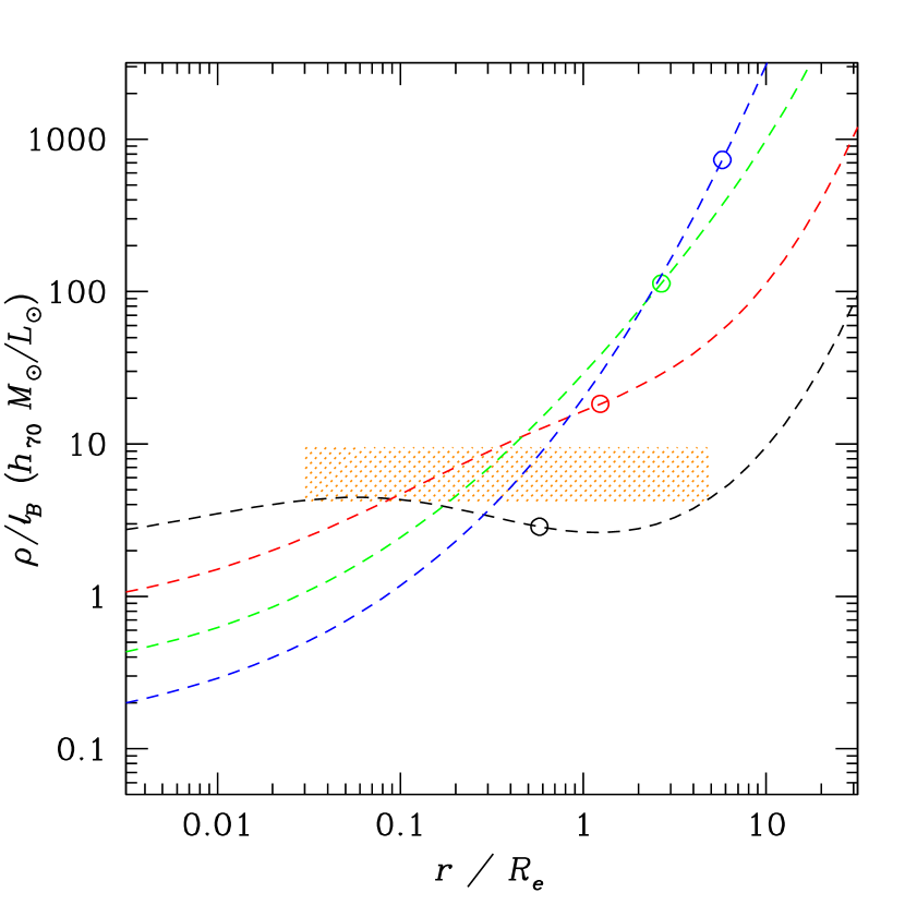
Figure 3: Same as Fig. 2 for high concentration parameters obtained from X-ray analyses by Sato et al. (2000) for the NFW model and for $L_{B}=4.1\times 10^{10}{\rm L_{\odot}}$ (the median luminosity of the 3 elliptical galaxies in their sample), yielding $m=3.7$ from equation (17) and $R_{e}=5.8\,h_{70}^{-1}\,\rm kpc$ from equation (16). The log masses are now 11.20, 12.20, 13.20 and 14.20 (respectively corresponding to $\Upsilon=3.9,39,390$, and 3900, i.e. 0.01, 0.1, 1, and 10 times the universal mass-to-light ratio of equation (20), and respectively black, red, green, and blue in the electronic version of the Journal) going downwards at small radii.

We plot in Fig. 3 the local mass-to-luminosity ratios for NFW models with the high concentration parameters of Sato et al. (eq. [35]) for the median blue luminosity $L_{B}=4.1\times 10^{10}\,{\rm L_{\odot}}$.

The local mass-to-light ratio profiles are increased in the inner regions, relative to the analogous profiles for the NFW model with the low concentration parameters as found in the cosmological $N$-body simulations. This is especially the case for low masses, which have the most centrally concentrated mass-density profiles. Nevertheless, the local mass-to-light ratio found with the high concentration parameter of Sato et al. is below the stellar value at all radii below $0.08\,R_{e}$, for the very large range of masses considered. But here, one could imagine dark matter profiles with somewhat steeper inner slopes well within 3% of $r_{v}$ that would produce local mass-to-light ratios in excess of the stellar value at all radii where the Sérsic model is a good fit to the surface brightness profile of ellipticals. The same conclusions are reached for the even higher concentration parameters extrapolated to the masses of ellipticals from the relations of Wu & Xue (2000) and Lloyd-Davies & Ponman.

To summarise, the low-concentration matter distributions found in cosmological $N$-body simulations produce local mass-to-light ratios lower than expected for stellar populations, unless there is a sharp steepening in the slopes of the mass density profiles just within an effective radius, while high-concentration NFW profiles would produce large enough local mass-to-light ratios if their inner slopes were slightly steeper.

These conclusions are unchanged if we vary the effective radius or the Sérsic shape ($m$) by a factor of 2.

3.2 Velocity dispersions

Another way to check the compatibility of NFW, JS–1.5 and Nav04 potentials with the Sérsic luminosity profiles of ellipticals is to compute the central stellar line-of-sight velocity dispersion, averaged within an aperture or a slit. In appendix B, we re-derive the stellar radial and line-of-sight velocity dispersion profiles, assuming isotropy, and derive for the first time the velocity dispersion profiles averaged in circular apertures and thin slits in terms of single quadratures of the tracer density and total mass profile.

Fig. 4 shows the resulting aperture and slit-averaged velocity dispersion profiles for Sérsic tracers and NFW, JS–1.5 and Nav04 mass profiles.

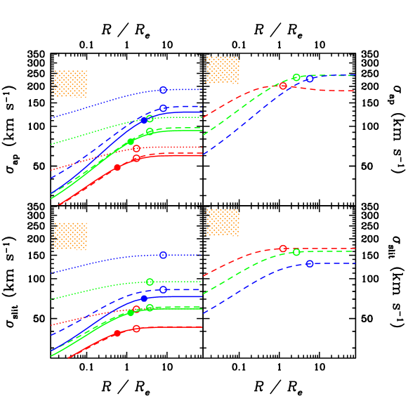
Figure 4: Stellar isotropic velocity dispersions, averaged over circular apertures of projected radius $R$ (top, eq. [59]) or thin slits of half-projected size $R$ (bottom, eq. [63]) for Sérsic luminosity profiles and CDM dark matter profiles: NFW (dashed curves), JS–1.5 (dotted curves) and Nav04 (solid curves). Left: low concentration parameters from cosmological simulations with total luminosity $L_{B}=L_{B}^{*}=1.88\times 10^{10}\,h_{70}^{-2}{\rm L_{\odot}}$ (corresponding to Sérsic parameters $m=3.1$ and $R_{e}=3.2\,h_{70}^{-1}\,\rm kpc$). Right: high concentration parameters from X-ray observations (eq. [35], NFW model only), with total luminosity $4.1\times 10^{10}\,h_{70}^{-2}{\rm L_{\odot}}$ ($m=3.7$ and $R_{e}=5.8\,h_{70}^{-1}\,\rm kpc$). Equations (9), (11), (33), (32), (36) and (37) are used. The cumulative mass-to-light ratios within the virial radius $r_{100}$ are 39, 390 and 3900 increasing upwards in the left plots and downwards in the right plots (red, green, and blue in the electronic version of the Journal). The shaded regions are the central observed velocity dispersions expected from the Faber-Jackson (1976) scaling relation, recalibrated by Bender et al. (1996, eq. [21]). The open circles represent $0.03\,r_{200}$, the minimum radius where the NFW and JS–1.5 models are accurate in representing the density profiles in structures found in cosmological $N$-body simulations, while the filled circles represent $0.01\,r_{200}$, which is the analogous radius for the Nav04 model.

The figure clearly shows that, if the total matter is represented by an NFW, JS–1.5, or Nav04 density models, with low concentration parameters as found in cosmological simulations, then the central aperture and slit velocity dispersions would be much smaller than observed. Indeed, the aperture and slit-averaged velocity dispersions both obey $\sigma_{v}<113\,\rm km\,s^{-1}$ for $R<0.1\,R_{e}$ (where the equality is reached for the more favourable JS–1.5 model), whereas one expects $\sigma_{v}=208\,\rm km\,s^{-1}$, from the Faber-Jackson scaling relation, recalibrated by Bender et al. (eq. [21]). For the most realistic Nav04 model, the velocity dispersions are 3.5 times too low for $R<0.1\,R_{e}$.

One might worry that this conclusion is reached through heavy extrapolation of the dark matter models at small radii. However, it is again difficult to imagine a dark matter model that would produce aperture or slit velocity dispersions that rise sharply (factor of 3 for the Nav04 model from 2 to $0.05\,R_{e}$) at increasingly small radii. Given the difference between the mass models of inner slope $-1$ (NFW) and $-3/2$ (JS–1.5), Fig. 4 suggests that an inner slope $<-2$ is required for the mass distribution to recover the high observed central velocity dispersions.

Note that the slit-averaged velocity dispersions are slightly smaller than the aperture-averaged ones, as is indeed expected given that, for the luminosity and mass models considered here, the line-of-sight velocity dispersions increase with radius for $R<R_{e}$, and the slit velocity dispersions are less weighted to outer radii than are the aperture velocity dispersions. Hence, the slit velocity dispersions are in principle more constraining against a global NFW, JS–1.5 or Nav04 potential. However, our quasi-analytical expressions for the slit velocity dispersion neglect the effects of seeing and are thus of little use at small radii. Moreover, at large radii observers subdivide their slit into rectangular bins, whose modelling is beyond the scope of this paper. We therefore, will focus on aperture velocity dispersions.

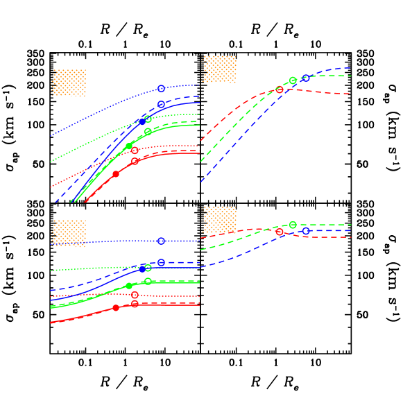
Figure 5: Same as the top plots of Fig. 4, for Sérsic shape parameter equal to twice ($m=6.2$ and 7.4, upper left and right plots, respectively) or half ($m=1.55$ and 1.85, lower left and right plots, respectively) of the values derived from eq. (17).

The high concentration parameters derived from X-ray observations produce higher central aperture and slit velocity dispersions, but these velocity dispersions are still well below the prediction of the Faber-Jackson relation: the NFW model produces slit velocity dispersions that are 1.5 times too low for $R<0.1\,R_{e}$ for all mass-to-light ratios below 3900 (10 times the universal value of eq. [20]).

As mentioned in Sec. 2.1, the Sérsic shape-luminosity relation is probably uncertain by a factor of perhaps 2 (Fig. 1). Fig. 5 shows the dispersion profiles when the Sérsic shape $m$ is taken to be twice (top plots) or half (bottom plots) the value given in equation (17). The higher Sérsic parameters favoured by Binggeli & Jerjen (1998) and Prugniel & Simien (1997) produce even lower velocity dispersions, and are thus even more constraining against the idea that the global potential of elliptical galaxies can be that of the $\Lambda$CDM simulations. And if one adopts a Sérsic shape parameter as low as $m=1.35$, as derived from the Márquez et al. data for the galaxies in Abell 85, one derives central aperture velocity dispersions that are almost large enough, but this requires the enormous mass-to-light ratio $\Upsilon_{B}=3900$, i.e. a total mass of over $3\times 10^{13}\,h_{70}^{-1}{\rm M_{\odot}}$, which is larger than that of a rich group. For the case of the high concentration parameter found in the X-rays, the aperture velocity dispersions are still too small, for all reasonable Sérsic parameters. Moreover, given that the de Vaucouleurs surface brightness profile ($m=4$) was derived for ellipticals of typically 0.5 to $1\,L_{*}$, we are very doubtful that a Sérsic parameter as low as $m=1.27$ is representative of fairly luminous elliptical galaxies.

Therefore, the internal kinematics of elliptical galaxies appear to be inconsistent with the total mass distribution as found in cosmological $N$-body simulations, even with the steep inner slope of $-3/2$ or the high concentration parameters found by X-ray observers.

3.3 Large concentration mass models as seen in X-rays

If the NFW model cannot represent the total density profile of elliptical galaxies, how can one explain that several X-ray studies converged on a high concentration parameter NFW total density profile?

The answer may be seen in Fig. 6, which shows the stellar (eqs. [6], [7], and [12]) and dark matter (eqs. [22], [26], [32], [33], and [34]) density profiles for the median luminosity ($L_{B}=4.1\,h_{70}^{-2}{\rm L_{\odot}}$) of the 3 elliptical galaxies in the sample of Sato et al. (2000), with effective radius and Sérsic shape parameter taken from equations (16) and (17), respectively, and for the mass that Sato et al. derived within the virial radius ($M_{v}=3.6\,h_{70}^{-1}\times 10^{12}\,{\rm M_{\odot}}$, leading to $\Upsilon_{B}=75$). Here, we fix the virial radius ($r_{v}=316\,h_{70}^{-1}\,\rm kpc$ from eq. [33]), and we fit the best NFW model to the density profile, within the limits shown as vertical lines in Fig. 6 (26 arcsec, set by the PSF of the ASCA telescope, and 25 arcmin, which is half the field of view of the GIS instrument on ASCA). With the median distance modulus of 31.34 (see Sect 3.1), these spatial limits respectively correspond to 2.3 and $129\,h_{70}^{-1}\,\rm kpc$, i.e., 0.0074 and 0.41 virial radii. Since Sato et al. fit their mass profiles with an NFW mass profile, we minimize the square differences in log mass over equally-spaced log radii.

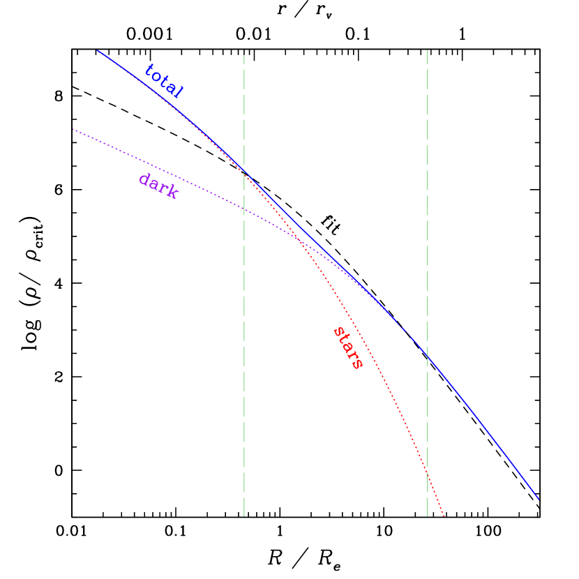
Figure 6: Density profiles: stars (dotted curve, $L_{B}=4.1\times 10^{10}\,h_{70}^{-2}{\rm L_{\odot}}$, $m=3.7$, $R_{e}=5.8\,h_{70}^{-1}\,\rm kpc$, $\Upsilon_{*,B}=8$), NFW-dark matter (dotted curve, $M_{v}=3.8\times 10^{12}\,h_{70}^{-1}{\rm M_{\odot}}$, $c=9.5$) and total (solid curve) and the NFW fit to the total density (dashed curve), with $c=35$. The vertical lines delimit the region of the fit (see text). The top abscissa are relative to $r_{200}$.

We find a high concentration parameter: $c=35$, although not as high as $c=49$, inferred from the general concentration vs. mass relation of Sato et al. (eq. [35]), and only half the value actually found by Sato et al. for these 3 galaxies (which were positive outliers on their global distribution of concentration as a function of mass). Moreover, using $\Upsilon_{*,B}=5$ instead of 8, the best-fitting concentration parameter (with the same quality fit as in Fig. 6) is reduced to $c=26$, still much higher than $c=9.5$ inferred from the cosmological simulations of Jing & Suto (eq. [34]) for NFW models with the mass inferred by Sato et al.. Note that the best fit, although adequate, is not superb, because the sum of the stellar and dark matter components presents an inflexion point at the radius where the two components contribute equally ($R\simeq 1.1$ and $1.4\,R_{e}$ for $\Upsilon_{*,B}=5$ and 8, respectively), in contrast with the NFW model, whose slope steepens continuously with increasing radius.

Hence, Fig. 6 tells us that fitting an NFW model to the total density represented by the sum of the NFW dark matter component and the less extended Sérsic stellar component can produce very high concentration parameters, but the fits are not excellent.

4 Summary and Discussion

Given what we know about the surface brightness profiles of elliptical galaxies, one can simply conclude that the observations of elliptical galaxies cannot allow NFW total density profiles with the fairly low concentration parameters as found in cosmological $N$-body simulations: otherwise one would end up with mass-to-light ratios far below stellar within an effective radius, and aperture and slit velocity dispersions would be far below the predictions from the isotropic Jeans equations. Trying a density profile with a steeper inner slope as advocated by Fukushige & Makino (1997) and Moore et al. (1999), using the model of Jing & Suto (2000), does not help, nor does the recent model by Navarro et al. (2004), nor probably the very similar mass model proposed by Stoehr and colleagues (Stoehr et al., 2002; Stoehr, 2005).

This conclusion of non-conformity of $\Lambda$CDM mass models with the Sérsic luminosity profile of elliptical galaxies is based upon the extrapolation of these mass models to radii smaller than the spatial resolution of the simulations. Nevertheless, the only way to bring the simulated mass models in conformity with the observations is for the slopes of the mass density profiles to sharply break around the effective radius from values $\simeq-1.3$ just outside $R_{e}$ to steeper values $<-2$ inside $R_{e}$, and it is hard to imagine that this sharp break in slope happens at the precise spatial resolution limit of present-day cosmological $N$-body simulations. This conclusion is independent of any assumed value for the stellar mass-to-light ratio (as are the curves in Figs. 2 and 3, as well as all of Figs. 4 and 5).

However, allowing for ten times larger concentration parameters, as motivated by several X-ray studies, makes the mass-to-light ratios and aperture/slit velocity dispersions almost in line with the observations, but not quite.

Assuming no sharp break in the slope of the total mass density profile to steeper than $-2$ inside $R_{e}$, we are left with an inconsistency of too low mass-to-light ratios and velocity dispersions of the inner regions. This inconsistency can disappear if we add more mass in these inner regions.

The simplest way to add more mass inside an NFW-like mass distribution is to postulate that this distribution only applies to the dark matter component and that the baryons, essentially stars, dominate the mass profile in the inner regions, as their Sérsic distribution has a steeper inner slope than the NFW-like models. In the following paper (Mamon & Łokas, 2005), we study in more detail multi-component models of elliptical galaxies.

Moreover, during the formation process of ellipticals, the NFW-like dark matter should dynamically respond to the dominant inner baryons. This process is often studied through the approximation of adiabatic contraction (Blumenthal et al., 1986). However, the dark matter response to the dominant presence of the stellar component will diminish as its local density approaches that of the stars. Therefore, the dark matter cannot dominate the stars inside, although it could conceivably reach non-negligible densities relative to the stellar component. In any event, as long as the inner slope of the dark matter density profile in elliptical galaxies is shallower than $-3/2$, it should be difficult to constrain its precise value in elliptical galaxies.

The very different mass distribution for the baryonic (mainly stellar) component has important ramifications. It suggests that present-day elliptical galaxies have not recently formed through rapid collapse, during which violent relaxation should lead to an efficient mixing of the baryon and dark matter components, especially if their initial distributions were similar (in the linear regime of small density fluctuations).

One alternative is that ellipticals form early by collapse, and the dissipative nature of the baryons slowly leads to a segregation with the dark matter, which in turn slowly responds to the contracting baryons by contracting itself. Gnedin et al. (2004) and Dekel et al. (2005) find dark matter density profiles scaling as $r^{-2}$ over a very large range of radii in their haloes and elliptical-galaxy-like merger remnants of their cosmological and two-galaxy $N$-body simulations, respectively. Although these findings may be inconsistent with several observational constraints of elliptical and spiral galaxies (perhaps because of insufficient feedback from star formation and AGN that pumps energy into the inner baryons, which should in turn puff up the inner dark matter distribution), they confirm our finding that the total mass density profile cannot be as shallow as predicted by the dissipationless $\Lambda$CDM mass models.

The other important alternative is the formation of elliptical galaxies (i.e. their morphologies, not their stars, which are thought to have formed earlier) through major mergers of spiral galaxies. Since spiral galaxies are initially gas-rich and form by dissipational collapse, a baryon / dark matter segregation sets in as the baryons settle in a disk, while the dark matter extends further out. When spiral galaxies of comparable mass merge into ellipticals, the baryons, which are more tightly bound than the dark matter particles, will end up in the inner regions of the elliptical merger remnant (e.g., Dekel, Devor, & Hetzroni, 2003; Dekel et al., 2005).

The second conclusion of this work is that considering a two component model for elliptical galaxies, summing up the mass density profiles of the Sérsic stellar component (with a reasonable mass-to-light ratio) and a dark matter component as seen in the $\Lambda$CDM dissipationless cosmological $N$-body simulations, one finds a total mass density profile that resembles an NFW model, with a concentration almost as high as deduced from X-ray observations, much higher than in $\Lambda$CDM haloes. Admittedly, the fit is not excellent.

This high concentration NFW total mass distribution is caused by the more extended nature of $\Lambda$CDM haloes in comparison with the stellar distribution of elliptical galaxies. It would be good if the X-ray observers attempt to fit NFW or better Nav04 models to the dark matter component of their elliptical galaxies or groups and not to the total mass density profile.

Note that recent modelling by Pratt & Arnaud (2005) of their XMM-Newton X-ray observations of poor and rich clusters of galaxies leads to the conclusion that the total mass density profile is consistent with NFW models of normal concentration, with the same shallow dependence on mass as seen in the cosmological $N$-body simulations. This result is in stark contrast with the strong dependence of concentration with mass found by Sato et al. (2000) from ellipticals to poor clusters to rich clusters.

One may venture that elliptical galaxies have a more prominent baryonic component in their inner regions than do groups and clusters of galaxies, and will thus, by superposition of Sérsic and $\Lambda$CDM components, appear more concentrated when fitted with single NFW models, than expected from the general trend of groups or clusters. However, Sato et al. find a continuous power-law trend for the mass dependence of their concentration parameters. In other words, Sato et al. find moderately high concentration parameters for groups of galaxies, as do Wu & Xue (2000) and Khosroshahi et al. (2004), suggesting an important baryonic contribution in their inner regions, albeit less dominant than in elliptical galaxies.

Interestingly, our best NFW model for the dark component of the 2-component model we try for the galaxies observed by Sato et al., has a concentration, $c\simeq 26$ to 35, that lies in between the very high value of Sato et al., $c\simeq 49$, and the low value expected from cosmological $N$-body simulations for objects of that virial mass, $c\simeq 9.5$. Additional measurements of concentration from X-ray observations of ellipticals should greatly clarify this issue.

In the following paper (Mamon & Łokas, 2005), we investigate in more detail a 4-component model, including stars, dark matter, hot gas and a central black hole, and ask whether the observations of ellipticals require cuspy cores, and to which accuracy one can measure the total mass within the virial radius through kinematic observations.

Appendix A Concentration, central density and outside mass versus virial mass for the Navarro et al. (2004) model

Navarro et al. (2004) have recently shown that the density profiles of haloes in cosmological $N$-body simulations begun with a $\Lambda$CDM spectrum can be fit to high precision to

$$\rho(r)=\rho_{-2}\,\exp(2\mu)\,\exp\left[-2\mu\,\left({r\over r_{-2}}\right)^{1/\mu}\right]\ ,$$ (39)

where our $\mu$ is the inverse of their $\alpha$ and where $\rho{{}_{2}}$ is the local mass density at the radius $r_{-2}$ where the logarithmic slope of the density is $-2$.

The enclosed mass of the density profile of equation (39) is

$$M(r)=4\pi\,\rho_{-2}\,r_{-2}^{3}\,2^{-3\mu}\,\mu^{1-3\mu}\,\exp(2\,\mu)\,\gamma\left[3\mu,2\mu\left({r\over r_{-2}}\right)^{1/\mu}\right]\ ,$$ (40)

where $\gamma(a,x)=\int_{0}^{x}t^{a-1}\,\exp(-t)\,dt$ is the incomplete gamma function. Navarro et al. (2004) provide a table of values of $1/\mu$, which for giant galaxy mass objects yield a geometric mean and median of $\langle\mu\rangle=5.85$ and $6.16$, respectively (and roughly the same for haloes with dwarf galaxy or galaxy cluster masses). We therefore adopt $\mu=6$.

The reader may note a resemblance to the enclosed luminosity of the Sérsic model given in equations (10) and (11), which may be related to the resemblance of the projected NFW model to the Sérsic profile noted by Łokas & Mamon (2001), and the value of $\mu$ is of the rough order of the Sérsic $m$’s (see Fig. 1).

Expressing the mean density at the virial radius $r_{v}=c\,r_{-2}$, one obtains

$${\rho_{-2}\over\rho_{\rm crit}}={2\,\Delta\over 3}\,\left(2\,\mu\right)^{3\mu-1}\,\exp(-2\mu)\,{c^{3}\over\gamma\left(3\mu,2\mu c^{1/\mu}\right)}\equiv f_{1}(c)\ .$$ (41)

Now, Navarro et al. provide a table with $\rho_{-2}/\rho_{\rm crit}$ and $r_{-2}$. We find that their data can be fitted by

$${\rho_{-2}\over\rho_{\rm crit}}\simeq\hbox{dex}\left[4.37-0.30\log\left({hr_{-2}\over 1\,{\rm kpc}}\right)-0.10\log^{2}\left({hr_{-2}\over 1\,{\rm kpc}}\right)\right]\equiv f_{2}\left({hr_{-2}\over 1\,{\rm kpc}}\right)\ .$$ (42)

We solve this 2nd order polynomial for $hr_{-2}/(1\,{\rm kpc})=f_{2}^{-1}(\rho_{-2}/\rho_{\rm crit})$. Equations (41) and (42) can be combined into an implicit equation for the concentration parameter $c$:

$$c\,f_{2}^{-1}\left[f_{1}(c)\right]=r_{v}\ .$$ (43)

Given that the virial radius is a function of the mass $M_{v}$ within the virial radius (eq. [33]), then for a given $M_{v}$, one can solve equation (43) for the concentration parameter. For $\mu=6$, we obtain

$$c\simeq 8.1\,M_{12}^{-0.11-0.015\,\log M_{12}}\,$$ (44)

where $M_{12}={hM_{v}/10^{12}{\rm M_{\odot}}}$.

Figure 7: Normalised density at scale radius versus scale radius for the Navarro et al. (2004) model. Circles: measurements by Navarro et al.; curve: predictions from our concentration parameter / mass approximation (eq. [44]) also using equations (33) and (41); numbers: $\log h_{70}\,M_{v}$.

Fig. 7 displays a check of equation (44): for every $M_{v}$, we obtain $c$ from equation (44), $\rho_{-2}/\rho_{\rm crit}$ from equation (41), but also $r_{v}$ from equation (33) and $r_{-2}=r_{v}/c$. The agreement is excellent and much better than if we had instead directly obtained $f_{2}^{-1}$ from a fit of $h\,r_{-2}/(1\,\rm kpc)$ as a function of $\rho_{-2}/\rho_{\rm crit}$.

The central density of the Nav04 model is

$$\rho_{0}\equiv\rho(0)=\rho_{-2}\,\exp(2\,\mu)$$ (45)

Using equation (41), equation (45) can be expressed in terms of the critical density

$${\rho_{0}\over\rho_{\rm crit}}={2\,\Delta\over 3}\,\left(2\,\mu\right)^{3\mu-1}\,{c^{3}\over\gamma\left(3\mu,2\mu\,c^{1/\mu}\right)}$$ (46)

and with equation (44), this yields

$$\log\left({\rho_{0}\over\rho_{\rm crit}}\right)\simeq 9.0-0.25\,\log M_{12}-0.030\,\log^{2}M_{12}\ .$$ (47)

Thus the central density decreases with increasing mass.

The mass of the Nav04 model converges at infinity, and the mass at the virial radius satisfies

$${M_{v}\over M_{\infty}}={\gamma(3\mu,2\mu\,c^{1/\mu})\over\Gamma(3\mu)}\simeq 0.44\,M_{12}^{-0.068-0.014\,\log M_{12}-0.0012\,\log^{2}M_{12}}\ ,$$ (48)

so that for giant galaxies a little over half the mass is beyond the virial radius, while for rich clusters more than 3/4 of the mass is beyond $r_{v}$.

Appendix B Line-of-sight, aperture and slit velocity dispersions of isotropic systems

B.1 Radial velocity dispersion

The Jeans equation is

$${{\rm d}(\ell\sigma_{r}^{2})\over{\rm d}r}+2\,{\beta(r)\over r}\,\ell\sigma_{r}^{2}=-\ell(r)\,{GM(r)\over r^{2}}\ ,$$ (49)

where the anisotropy parameter is $\beta=1-\sigma_{r}^{2}/\sigma_{t}^{2}$, with $\sigma_{t}=\sigma_{\theta}=\sigma_{\phi}$ the 1D tangential velocity dispersion, so that $\beta=0$ corresponds to isotropy, $\beta=1$ is fully radial anisotropy, and $\beta\to-\infty$ is fully tangential anisotropy.

For isotropic orbits, the Jeans equation (49) trivially leads to

$${\ell(r)\,\sigma_{r}^{2}(r)\over G}=\int_{r}^{\infty}\ell\,M\,\left({{\rm d}s\over s^{2}}\right)\ .$$ (50)

B.2 Line-of-sight velocity dispersion

Projecting along the line-of-sight, one trivially finds that the line-of-sight velocity dispersion is

$$I(R)\,\sigma_{\rm los}^{2}(R)=2\,\int_{R}^{\infty}{\ell\sigma_{r}^{2}\,r\,{\rm d}r\over\sqrt{r^{2}\!-\!R^{2}}}\ .$$ (51)

Inserting equation (50) into equation (51), and inverting the order of integration, one easily finds (Prugniel & Simien 1997):

$$I(R)\,\sigma_{\rm los}^{2}(R)=2\,G\,\int_{R}^{\infty}{\sqrt{r^{2}\!-\!R^{2}}\over r^{2}}\ \ell(r)\,M(r)\,{\rm d}r\ .$$ (52)

Writing $M(r)=M_{v}\,\widetilde{M}(r/a_{S})$, $x=r/a_{S}$, $x_{v}=r_{v}/a_{S}$, $\eta=a_{S}/a_{h}$, the deprojected luminosity $\widetilde{L}_{3}$ of the Sérsic profile is given in equation (11), the isotropic velocity dispersion, derived from equation (52), using equations (1), (6), (7), (8), and (36) becomes

$$\sigma_{\rm los}^{2}(R)={\Gamma(2m)\over\Gamma[(3\!-\!p)m]}\,{r_{v}\over a_{S}}\,V_{v}^{2}\,\exp\left(X^{1/m}\right)\int_{X}^{\infty}{\sqrt{x^{2}\!-\!X^{2}}\over x^{2}}\ \widetilde{\ell}(x)\,\widetilde{M}(x)\,{\rm d}x\ ,$$ (53)

where$V_{v}^{2}=GM_{v}/r_{v}$ is the squared circular velocity at the virial radius and again $X=R/a_{S}$.

B.3 Aperture velocity dispersion

The aperture velocity dispersion satisfies

$$L_{2}(R)\,\sigma_{\rm ap}^{2}(R)=\int_{0}^{R}2\pi\,S\,I(S)\,\sigma_{\rm los}^{2}(S)\,{\rm d}S\ ,$$ (54)

where $L_{2}(R)=\int_{0}^{R}2\pi SI(S)\,{\rm d}S$ is the luminosity within projected radius $R$. Inserting $I\sigma_{\rm los}^{2}$ from equation (52) into equation (54), again inverting the order of integration, we obtain the isotropic solution for the aperture velocity dispersion:

$$\sigma_{\rm ap}^{2}(R) = {4\pi\,G\over{\color[rgb]{1,0,0}3}\,L_{2}(R)}\,\left[\int_{0}^{\infty}r\,\ell(r)M(r)\,{\rm d}r-\int_{R}^{\infty}{(r^{2}\!-\!R^{2})^{3/2}\over r^{2}}\,\ell(r)M(r)\,{\rm d}r\right]$$ (55)

$$= {L\over L_{2}(R)}\,\sigma_{\rm tot}^{2}-{4\pi\,G\over 3\,L_{2}(R)}\,\int_{R}^{\infty}{\left(r^{2}\!-\!R^{2}\right)^{3/2}\over r^{2}}\,\ell(r)\,M(r)\,{\rm d}r\ ,$$ (56)

which, in the limit $R\to\infty$, converges to the (one-dimensional) isotropic velocity dispersion, averaged over the entire galaxy:

$$\sigma_{\rm tot}^{2}={4\pi\,G\over 3\,L}\,\int_{0}^{\infty}r\,\ell(r)\,M(r)\,{\rm d}r\ .$$ (57)

Using the formula for the projected luminosity of the Sérsic profile (Graham & Colless, 1997; Binggeli & Jerjen, 1998; Lima Neto et al., 1999)

$$L_{2}(R)=2\pi\,m\,I_{0}\,a_{S}^{2}\,\gamma\left[2m,\left({R\over a_{S}}\right)^{1/m}\right]\ ,$$ (58)

the isotropic aperture velocity dispersion at radius $R=X\,a_{S}$ (eq. [56]), together with equations (6), (7), (8), (10), (36), and (58) yields

$$\sigma_{\rm ap}^{2}(R) = {\Gamma(2m)/\Gamma[(3\!-\!p)\,m]\over 3\,m\,\gamma\left(2m,X^{1/m}\right)}\,{r_{v}\over a_{S}}\,V_{v}^{2}\left\{\int_{0}^{\infty}\!\!x\,\widetilde{\ell}(x)\,\widetilde{M}(x)\,{\rm d}x-\int_{X}^{\infty}{\left(x^{2}\!-\!X^{2}\right)^{3/2}\over x^{2}}\,\widetilde{\ell}(x)\,\widetilde{M}(x)\,{\rm d}x\right\}\ .$$ (59)

For the numerical integration of equation (59), the first integral can be evaluated by integrating along $\ln x$ in the range $[-20,\ln x_{\rm max}]$, where $x_{\rm max}=50^{m}$, for which the exponential term in $\widetilde{\ell}(x)$ is extremely small. The other integrals can be numerically evaluated by integrating $\ln(x/X)$ in the range $[0,\ln(x_{\rm max}/X)]$. In this paper, we evaluate numerically all velocity dispersions using Mathematica.

B.4 Slit-averaged velocity dispersion

The velocity dispersion averaged over a thin slit of width $R$ is

$$\sigma_{\rm slit}^{2}(R)={\int_{0}^{R}I(S)\,\sigma_{\rm los}^{2}(S)\,{\rm d}S\over\int_{0}^{R}I(S)\,{\rm d}S}\ .$$ (60)

With $J(R)=\int_{0}^{R}I(S)\,{\rm d}S$, equation (60) becomes

$${J(R)\,\sigma_{\rm slit}^{2}(R)\over G} = 2\,\int_{0}^{R}{\rm d}S\,\int_{S}^{\infty}\ell\,M\,\sqrt{r^{2}\!-\!S^{2}}\,{{\rm d}r\over r^{2}}$$ (61)

$$= {\pi\over 2}\,\int_{0}^{R}\ell(r)\,M(r)\,{\rm d}r+R\,\int_{R}^{\infty}\ell(r)\,M(r)\,\sqrt{r^{2}\!-\!R^{2}}\,{{\rm d}r\over r^{2}}+\int_{R}^{\infty}\ell(r)\,M(r)\,\sin^{-1}\left({R\over r}\right)\,{\rm d}r\ ,$$

where the second equality in equation (61) was obtained after inverting the order of integration in the first equality. With equation (1), one has

$$J(R)=m\,I_{0}\,a_{S}\,\gamma\left[m,\left({R\over a_{S}}\right)^{1/m}\right].$$ (62)

The isotropic slit velocity dispersion (eq. [61]) becomes, with equations (6), (7), (8), (36), and (62),

$$\sigma_{\rm slit}^{2}(R) = {\Gamma(2m)/\Gamma[(3\!-\!p)\,m]\over 2\,m\,\gamma\left(m,X^{1/m}\right)}\,{r_{v}\over a_{S}}\,V_{v}^{2}$$ (63)

$$\times\left\{{\pi\over 2}\,\int_{0}^{X}\widetilde{\ell}(x)\,\widetilde{M}(x)\,\,{\rm d}x+X\,\int_{X}^{\infty}{\sqrt{x^{2}\!-\!X^{2}}\over x^{2}}\,\widetilde{\ell}(x)\,\widetilde{M}(x)\,{\rm d}x+\int_{X}^{\infty}\sin^{-1}\left({X\over x}\right)\ \widetilde{\ell}(x)\,\widetilde{M}(x)\,{\rm d}x\right\}\ ,$$

where $X=R/a_{S}$. The last two integrals are easily evaluated numerically with the substitution $x=X/\sin u$.

References

- Arnaud et al. (2002) Arnaud M., Majerowicz S., Lumb D., Neumann D. M., Aghanim N., Blanchard A., Boer M., Burke D. J., Collins C. A., Giard M., Nevalainen J., Nichol R. C., Romer A. K., Sadat R., 2002, A&A, 390, 27
- Bender et al. (1996) Bender R., Ziegler B., Bruzual G., 1996, ApJ, 463, L51
- Bertin et al. (2002) Bertin G., Ciotti L., Del Principe M., 2002, A&A, 386, 149
- Bertola et al. (1993) Bertola F., Pizzella A., Persic M., Salucci P., 1993, ApJ, 416, L45
- Binggeli & Jerjen (1998) Binggeli B., Jerjen H., 1998, A&A, 333, 17
- Blair & Gilmore (1982) Blair M., Gilmore G., 1982, PASP, 94, 742
- Blanton et al. (2003) Blanton M. R., Hogg D. W., Bahcall N. A., Brinkmann J., Britton M., Connolly A. J., Csabai I., Fukugita M., Loveday J., Meiksin A., Munn J. A., Nichol R. C., Okamura S., Quinn T., Schneider D. P., Shimasaku K., Strauss M. A., Tegmark M., Vogeley M. S., Weinberg D. H., 2003, ApJ, 592, 819
- Blumenthal et al. (1986) Blumenthal G. R., Faber S. M., Flores R., Primack J. R., 1986, ApJ, 301, 27
- Borriello et al. (2003) Borriello A., Salucci P., Danese L., 2003, MNRAS, 341, 1109
- Brown & Bregman (2001) Brown B. A., Bregman J. N., 2001, ApJ, 547, 154
- Bruzual & Charlot (2003) Bruzual G., Charlot S., 2003, MNRAS, 344, 1000
- Bryan & Norman (1998) Bryan G. L., Norman M. L., 1998, ApJ, 495, 80
- Bullock et al. (2001) Bullock J. S., Kolatt T. S., Sigad Y., Somerville R. S., Kravtsov A. V., Klypin A. A., Primack J. R., Dekel A., 2001, MNRAS, 321, 559
- Buote et al. (2002) Buote D. A., Jeltema T. E., Canizares C. R., Garmire G. P., 2002, ApJ, 577, 183
- Caon et al. (1993) Caon N., Capaccioli M., D’Onofrio M., 1993, MNRAS, 265, 1013
- Colina et al. (1996) Colina L., Bohlin R. C., Castelli F., 1996, AJ, 112, 307
- de Vaucouleurs (1948) de Vaucouleurs G., 1948, Annales d’Astrophysique, 11, 247
- de Vaucouleurs & Olson (1982) de Vaucouleurs G., Olson D. W., 1982, ApJ, 256, 346
- Dekel et al. (2003) Dekel A., Devor J., Hetzroni G., 2003, MNRAS, 341, 326
- Dekel et al. (2005) Dekel A., Stoehr F., Mamon G. A., Cox T. J., Primack J. R., 2005, Nature, submitted, arXiv:astro-ph/0501622
- Diemand et al. (2004) Diemand J., Moore B., Stadel J., 2004, MNRAS, 353, 624
- Djorgovski & Davis (1987) Djorgovski S., Davis M., 1987, ApJ, 313, 59
- D’Onofrio (2001) D’Onofrio M., 2001, MNRAS, 326, 1517
- Dressler et al. (1987) Dressler A., Lynden-Bell D., Burstein D., Davies R. L., Faber S. M., Terlevich R., Wegner G., 1987, ApJ, 313, 42
- Eke et al. (1996) Eke V. R., Cole S., Frenk C. S., 1996, MNRAS, 282, 263
- Faber & Jackson (1976) Faber S. M., Jackson R. E., 1976, ApJ, 204, 668
- Fabricant et al. (1980) Fabricant D., Lecar M., Gorenstein P., 1980, ApJ, 241, 552
- Fioc & Rocca-Volmerange (1997) Fioc M., Rocca-Volmerange B., 1997, A&A, 326, 950
- Forbes & Ponman (1999) Forbes D. A., Ponman T. J., 1999, MNRAS, 309, 623
- Freedman et al. (2001) Freedman W. L., Madore B. F., Gibson B. K., Ferrarese L., Kelson D. D., Sakai S., Mould J. R., Kennicutt R. C., Ford H. C., Graham J. A., Huchra J. P., Hughes S. M. G., Illingworth G. D., Macri L. M., Stetson P. B., 2001, ApJ, 553, 47
- Fukugita et al. (1995) Fukugita M., Shimasaku K., Ichikawa T., 1995, PASP, 107, 945
- Fukushige et al. (2004) Fukushige T., Kawai A., Makino J., 2004, ApJ, 606, 625
- Fukushige & Makino (1997) Fukushige T., Makino J., 1997, ApJ, 477, L9
- Gerhard et al. (2001) Gerhard O., Kronawitter A., Saglia R. P., Bender R., 2001, AJ, 121, 1936
- Gerhard (1993) Gerhard O. E., 1993, MNRAS, 265, 213
- Ghigna et al. (2000) Ghigna S., Moore B., Governato F., Lake G., Quinn T., Stadel J., 2000, ApJ, 544, 616
- Gnedin et al. (2004) Gnedin O. Y., Kravtsov A. V., Klypin A. A., Nagai D., 2004, ApJ, 616, 16
- Graham & Colless (1997) Graham A., Colless M., 1997, MNRAS, 287, 221
- Graham (1998) Graham A. W., 1998, MNRAS, 295, 933
- Graham & Guzmán (2003) Graham A. W., Guzmán R., 2003, AJ, 125, 2936
- Jensen et al. (2003) Jensen J. B., Tonry J. L., Barris B. J., Thompson R. I., Liu M. C., Rieke M. J., Ajhar E. A., Blakeslee J. P., 2003, ApJ, 583, 712
- Jing & Suto (2000) Jing Y. P., Suto Y., 2000, ApJ, 529, L69
- Jones et al. (1997) Jones C., Stern C., Forman W., Breen J., David L., Tucker W., Franx M., 1997, ApJ, 482, 143
- Katgert et al. (2004) Katgert P., Biviano A., Mazure A., 2004, ApJ, 600, 657
- Kauffmann et al. (1999) Kauffmann G., Colberg J. M., Diaferio A., White S. D. M., 1999, MNRAS, 303, 188
- Khosroshahi et al. (2004) Khosroshahi H. G., Jones L. R., Ponman T. J., 2004, MNRAS, 349, 1240
- King (1962) King I., 1962, AJ, 67, 471
- King (1966) King I. R., 1966, AJ, 71, 64
- Kitayama & Suto (1996) Kitayama T., Suto Y., 1996, ApJ, 469, 480
- Kormendy et al. (1997) Kormendy J., Bender R., Magorrian J., Tremaine S., Gebhardt K., Richstone D., Dressler A., Faber S. M., Grillmair C., Lauer T. R., 1997, ApJ, 482, L139
- Lima Neto et al. (1999) Lima Neto G. B., Gerbal D., Márquez I., 1999, MNRAS, 309, 481
- Liske et al. (2003) Liske J., Lemon D. J., Driver S. P., Cross N. J. G., Couch W. J., 2003, MNRAS, 344, 307
- Lloyd-Davies et al. (2002) Lloyd-Davies E., Bower R. G., Ponman T. J., 2002, MNRAS, submitted, arXiv:astro-ph/0203502
- Lloyd-Davies & Ponman (2002) Lloyd-Davies E., Ponman T. J., 2002, unpublished preprint
- Łokas & Hoffman (2001) Łokas E., Hoffman Y., 2001, in The Identification of Dark Matter, Spooner N. J. C., Kudryavtsev V., eds., World Scientific, Singapore, pp. 121–126, arXiv:astro-ph/0011295
- Łokas & Mamon (2001) Łokas E. L., Mamon G. A., 2001, MNRAS, 321, 155
- Łokas & Mamon (2003) —, 2003, MNRAS, 343, 401
- Márquez et al. (2000) Márquez I., Lima Neto G. B., Capelato H., Durret F., Gerbal D., 2000, A&A, 353, 873
- Mamon (1992) Mamon G. A., 1992, ApJ, 401, L3
- Mamon & Łokas (2005) Mamon G. A., Łokas E. L., 2005, MNRAS, submitted
- Marinoni & Hudson (2002) Marinoni C., Hudson M. J., 2002, ApJ, 569, 101
- McElroy (1995) McElroy D. B., 1995, ApJS, 100, 105
- Merritt (1987) Merritt D., 1987, ApJ, 313, 121
- Merritt et al. (2005) Merritt D., Navarro J. F., Ludlow A., Jenkins A., 2005, ApJ, 624, L85
- Moore et al. (1999) Moore B., Quinn T., Governato F., Stadel J., Lake G., 1999, MNRAS, 310, 1147
- Navarro et al. (1995) Navarro J. F., Frenk C. S., White S. D. M., 1995, MNRAS, 275, 720
- Navarro et al. (1996) —, 1996, ApJ, 462, 563
- Navarro et al. (1997) —, 1997, ApJ, 490, 493
- Navarro et al. (2004) Navarro J. F., Hayashi E., Power C., Jenkins A. R., Frenk C. S., White S. D. M., Springel V., Stadel J., Quinn T. R., 2004, MNRAS, 349, 1039
- Norberg et al. (2002) Norberg P., Cole S., Baugh C. M., Frenk C. S., Baldry I., Bland-Hawthorn J., Bridges T., Cannon R., Colless M., Collins C., Couch W., Cross N. J. G., Dalton G., De Propris R., Driver S. P., Efstathiou G., Ellis R. S., Glazebrook K., Jackson C., Lahav O., Lewis I., Lumsden S., Maddox S., Madgwick D., Peacock J. A., Peterson B. A., Sutherland W., Taylor K., 2002, MNRAS, 336, 907
- Power et al. (2003) Power C., Navarro J. F., Jenkins A., Frenk C. S., White S. D. M., Springel V., Stadel J., Quinn T., 2003, MNRAS, 338, 14
- Pratt & Arnaud (2002) Pratt G. W., Arnaud M., 2002, A&A, 394, 375
- Pratt & Arnaud (2005) —, 2005, A&A, 429, 791
- Prugniel & Simien (1996) Prugniel P., Simien F., 1996, A&A, 309, 749
- Prugniel & Simien (1997) —, 1997, A&A, 321, 111
- Reynolds (1913) Reynolds J. H., 1913, MNRAS, 74, 132
- Rix & White (1992) Rix H., White S. D. M., 1992, MNRAS, 254, 389
- Salpeter (1955) Salpeter E. E., 1955, ApJ, 121, 161
- Sato et al. (2000) Sato S., Akimoto F., Furuzawa A., Tawara Y., Watanabe M., Kumai Y., 2000, ApJ, 537, L73
- Sersic (1968) Sersic J. L., 1968, Atlas de galaxias australes. Cordoba, Argentina: Observatorio Astronomico, 1968
- Stoehr (2005) Stoehr F., 2005, MNRAS, submitted, arXiv:astro-ph/0403077
- Stoehr et al. (2002) Stoehr F., White S. D. M., Tormen G., Springel V., 2002, MNRAS, 335, L84
- Tonry et al. (2001) Tonry J. L., Dressler A., Blakeslee J. P., Ajhar E. A., Fletcher A. B., Luppino G. A., Metzger M. R., Moore C. B., 2001, ApJ, 546, 681
- Toomre (1977) Toomre A., 1977, in The Evolution of Galaxies and Stellar Populations, Tinsley B. M., Larson R. B., eds., Yale University Press, New Haven, pp. 401–416
- Trujillo et al. (2004) Trujillo I., Burkert A., Bell E. F., 2004, ApJ, 600, L39
- van der Marel & Franx (1993) van der Marel R. P., Franx M., 1993, ApJ, 407, 525
- Worthey (1994) Worthey G., 1994, ApJS, 95, 107
- Wu & Xue (2000) Wu X., Xue Y., 2000, ApJ, 529, L5
- Yang et al. (2003) Yang X., Mo H. J., van den Bosch F. C., 2003, MNRAS, 339, 1057
- Young & Currie (1994) Young C. K., Currie M. J., 1994, MNRAS, 268, L11