Fast and reliable MCMC for cosmological parameter estimation

Abstract

Markov Chain Monte Carlo (MCMC) techniques are now widely used for cosmological parameter estimation. Chains are generated to sample the posterior probability distribution obtained following the Bayesian approach. An important issue is how to optimize the efficiency of such sampling and how to diagnose whether a finite-length chain has adequately sampled the underlying posterior probability distribution. We show how the power spectrum of a single such finite chain may be used as a convergence diagnostic by means of a fitting function, and discuss strategies for optimizing the distribution for the proposed steps. The methods developed are applied to current CMB and LSS data interpreted using both a pure adiabatic cosmological model and a mixed adiabatic/isocurvature cosmological model including possible correlations between modes. For the latter application, because of the increased dimensionality and the presence of degeneracies, the need for tuning MCMC methods for maximum efficiency becomes particularly acute.

1 Introduction

The availability of high quality data from both CMB (Hinshaw et al.; Kogut et al. 2003) and large-scale structure (Percival et al. 2001; Tegmark et al. 2003) experiments has allowed the field of precision cosmology to advance rapidly in the last few years. Methods of cosmological parameter estimation are allowing us to narrow down the range of possible universes by placing bounds on the parameters describing a particular model. Because many of the models have a large number of parameters, ranging in complexity from the simplest scale-invariant $\Lambda$CDM cosmology to those including spatial curvature, massive neutrinos, a dark energy equation of state, cosmic strings, or a non-adiabatic contribution, it has become commonplace to use Markov Chain Monte Carlo (MCMC) methods to explore the probability distributions of high dimensionality obtained following Bayesian statistics.

MCMC methods were first introduced in the 1950s (Metropolis et al. 1953) to sample an unknown probability distribution efficiently and are described in detail in Neal (1993) and in Gilks, Richardson & Spiegelhalter (1995). Instead of calculating the probability density at sites on a regular grid spanning the entire parameter space, one draws samples sequentially according to a probabilistic algorithm. The sequence of states visited forms a Markov Chain distributed according to the probability distribution to be explored. Rather than scaling exponentially with the number of parameters varied, the time needed to sample a distribution grows approximately linearly with dimension. For this reason MCMC methods are particularly useful for cosmological parameter estimation. This application has explicitly been discussed by Christensen et al. (2001), Knox, Christensen & Skordis (2001), Lewis & Bridle (2002), Verde et al. (2003), Tegmark et al. (2003) and others.

All MCMC algorithms share the property that asymptotically the distribution of states visited by the chain is identical to the underlying distribution. However, it is critical to be able to determine whether and to what extent a finite length chain is a fair sample and can be used to make confident and accurate estimates of statistics characterizing the underlying distribution. This idea of ‘convergence’ to a stationary distribution has been discussed extensively in the statistical literature (see e.g. Cowles & Carlin 1996 for a review), and there exist a range of convergence tests that can be applied to MCMC output, many of which are described in the coda manual (Best, Cowles & Vines 1995). Both Heidelberger & Welch (1981,1985) and Geweke (1992) use spectral methods to determine the total running length of a simulation and the length of an initial transient to be discarded. Gelman & Rubin (1992) study the dispersion of the means of multiple chains, while Raftery & Lewis (1992) use second order Markov chains to insure that percentiles are estimated within a given accuracy. In the cosmological context, the package of coda tests were first applied by Christensen et al. (2001), with the Gelman & Rubin test further explored by Verde et al. (2003) and included with the Raftery & Lewis test in the cosmomc package (Lewis & Bridle 2002). Methods for speeding up the convergence have been considered by Slosar & Hobson (2003), in the cosmomc package and by Doran & Mueller (2003).

Here we describe a convergence test for MCMC methods that we have tested and found to work well for several CMB parameter estimation problems. The test tells us when one can stop running the MCMC chain and use it to estimate statistics of the underlying distribution. We draw upon various techniques incorporated in existing convergence analyses, studying the spectral behaviour generic to chains generated with the Metropolis algorithm.

This article is organized as follows. Section 2 reviews the Metropolis algorithm and section 3 defines the convergence of a chain. Section 4 formulates a spectral convergence test based on fitting to a template, which we have empirically found to work well, to the sample power spectra of finite length chains. This section demonstrates the effectiveness of the proposed spectral test using Gaussian distributions of various dimensions and differing ratios of the covariance of the trial distribution to that of the underlying distribution. Section 5 explores how to optimize the trial distribution for the proposed steps, tailoring its covariance to that of the underlying distribution. In section 6 we investigate what can go wrong, considering various non-Gaussian distributions, ranging from mildly non-Gaussian to more pathological. Section 7 summarizes our method in the form of an explicit ‘recipe,’ which is then applied to CMB+LSS data in section 8. Finally, we conclude with a discussion in section 9.

2 The Metropolis Algorithm

The Metropolis algorithm, used to sample a probability distribution $p(x)$ in one dimension, works as follows. Starting at an initial position $x_{0}$, we generate a sequence of points $x_{1},x_{2},\ldots$ according to the following rule. $x_{i+1}$ is generated from $x_{i}$ by attempting a trial step $x_{trial}$ distributed according to a trial distribution $q_{trial}(x_{trial},x_{i}),$ typically but not always chosen with the special form $q_{trial}(x_{trial},x_{i})=q_{trial}(x_{trial}-x_{i}).$ The trial distribution must be symmetric and chosen such that all points with $p(x)\neq 0$ can be connected by the chain. Because of considerations of detailed balance, the symmetry of $q_{trial}$ ensures that $p(x)$ is stationary under the Markov process. We shall typically use for $q_{trial}(x_{trial}-x_{i})$ a Gaussian of vanishing mean and adjustable variance $\sigma^{2}_{T}.$ If $P_{R}=p(x_{trial})/p(x_{i})\geq 1$, then $x_{i+1}$ is set to $x_{trial}$ with probability one. Otherwise, $x_{i+1}$ is set to $x_{trial}$ with probability $P_{R}$ and to $x_{i}$ with probability $(1-P_{R})$. If the chain moves to $x_{trial},$ the step has been ‘accepted’. Otherwise, we say that it has been rejected. The correlated chain of steps $x_{i}$ explores the full range of the sample space spanned by $p(x)$ such that eventually, in the infinitely long chain limit, the distribution of points visited is exactly described by the distribution $p(x)$. Most of the time is spent exploring regions of high likelihood, but all regions where $p(x)$ is non-zero are eventually explored.

To sample a $D$-dimensional distribution $p({\mn@boldsymbol{x}})$ using the Metropolis algorithm, $x_{trial}$ is replaced by ${\mn@boldsymbol{x}}_{trial}$, where $(\mn@boldsymbol{x}_{trial}-\mn@boldsymbol{x}_{i})$ is distributed according to a multivariate Gaussian of zero mean and covariance matrix ${\mn@boldsymbol{C}}_{T}$. This $D$-dimensional step ${\mn@boldsymbol{x}}_{trial}$ can be drawn from a Gaussian distribution of non-diagonal covariance by drawing $D$ Gaussian random samples ${\mn@boldsymbol{y}}$ with unit variance and generating ${\mn@boldsymbol{x}}_{trial}={\mn@boldsymbol{C}}^{-1/2}_{T}{\mn@boldsymbol{y}},$ where ${\mn@boldsymbol{C}}^{-1/2}_{T}$ is the positive definite matrix square root.

3 Defining Convergence

The distribution of points visited by the infinite MCMC chain described above is described exactly by the underlying probability density $p(x)$. Statistical properties of the distribution such as the mean, median, and quantiles can therefore be calculated directly from the chain. In practice, one must use a chain of finite length to estimate these statistical properties of the underlying distribution. Errors arise from the truncation to a finite chain both because of shot noise and because of correlations between successive elements of the chain. Following the literature, we shall say that a finite chain has ‘converged’ when its statistical properties, suitably defined, reflect those of the underlying distribution $p(x)$ with ‘sufficient accuracy’ that the chain can be terminated. To determine whether convergence has been achieved requires answering the following two questions:

1. Has the chain fully traversed the region of high probability in such a way that the correlations between successive elements of the chain does not bias the inferred distribution for $p(x)$? Apart from shot noise, a chain that is too short may explore only a single peak or portion of a single peak where $p(x)$ is significant.

2. Can we then estimate suitably defined statistics about the underlying distribution $p(x)$ with sufficient accuracy?

In the next Section we show how to extract from a single chain the information about the large-scale correlations of the chain that indicate whether the first requirement above has been satisfied. To address the second question, a level of accuracy for a given statistic must be specified. Let $\mu$ and $\sigma^{2}_{0}$ be the mean and variance of the underlying distribution $p(x),$ respectively. A useful diagnostic is the variation of the sample means $\bar{x}$ obtained from a finite chain. Let $\sigma_{\bar{x}}^{2}(N)$ indicate the variance of the sample mean, defined by averaging over independent realizations of a finite chain of length $N.$ We assume a starting point determined according to the underlying distribution, in other words that any initial transients of the chain have decayed away. The variance in the sample mean may be characterized by the dimensionless ratio

$$r={\sigma_{\bar{x}}^{2}\over\sigma_{0}^{2}},$$ (1)

which we shall call the ‘convergence ratio’. We require $r$ to lie below some cutoff value, chosen for example to be $0.01$. The sample mean variance has been used in various ways in the literature as a diagnostic of convergence, as outlined in Cowles & Carlin (1994). Heidelberger & Welch calculate confidence intervals on the mean using the ratio $\sigma_{\bar{x}}/{\bar{x}}$, but do not use the distribution variance. The Gelman & Rubin test incorporates a similar ratio: their $R$ statistic roughly translates to $R\sim 1+r$, but the quantity is calculated using multiple parallel chains. In the next section we show how to estimate the convergence ratio $r$ from a single chain.

If a chain is started far outside the region of high probability, an initial section of the chain consisting of steady progression into this region will be unrepresentative of the underlying distribution and must be discarded. In the literature this initial transient has been dubbed ‘burn-in.’ We use the ratio of the probability $p$ compared to the maximum $p_{max}$ as an indicator of how much of the beginning of the chain to chop out, for example while $p/p_{max}<0.1$. Such truncation is unnecessary if the chain is started from a point already known to lie in the region of high probability, for example from an earlier chain.

4 Spectral analysis of MCMC chains

An infinite one-dimensional Gaussian random chain for which the underlying statistical process is independent of position may be expanded into Fourier coefficients according to

$$x_{n}=\int_{-\pi}^{+\pi}{dk\over\sqrt{2\pi}}~{}\tilde{x}(k)~{}e^{ikn},$$ (2)

where the reality of the $x_{n}$ implies that $\tilde{x}(k)=\tilde{x}^{*}(-k).$ The two-point correlations can be characterized in terms of the Fourier coefficients

$$\langle\tilde{x}(k)~{}\tilde{x}^{*}(k^{\prime})\rangle=\delta(k-k^{\prime})~{}P(k),$$ (3)

where the power spectrum $P(k)$ is an even function. Any correlation linking unequal $k$ and $k^{\prime}$ would contradict the hypothesis of position independence.

We may define the two-point autocorrelation (i.e., the chain variance)

$$C_{0}=\langle x_{n}^{2}\rangle=\int_{-\pi}^{+\pi}{dk\over 2\pi}~{}P(k),$$ (4)

giving an average measure of the power spectrum. Similarly, the correlation with an offset $N$ is given by

$$C_{N}=\langle x_{n}~{}x_{n+N}\rangle=\int_{-\pi}^{+\pi}{dk\over 2\pi}~{}P(k)~{}\cos(kN).$$ (5)

We consider the sample mean

$${\bar{x}}_{N}={1\over N}\sum_{n=0}^{N-1}x_{n},$$ (6)

the variance of which is given by

$$\left<{{\bar{x}}_{N}}^{2}\right>={1\over N}\int_{-\pi}^{+\pi}{dk\over 2\pi N}~{}{\sin^{2}[Nk/2]\over\sin^{2}[k/2]}~{}P(k)$$ (7)

for a chain with zero mean. Since for all integers $N>0,$

$$\int_{-\pi}^{+\pi}{dk\over 2\pi N}~{}{\sin^{2}[Nk/2]\over\sin^{2}[k/2]}=1,$$ (8)

eqn. (7) is a weighted average of $P(k)$ that becomes more and more concentrated around $k=0$ as $N$ becomes large. Because

$$\lim_{N\to\infty}{1\over 2\pi N}{\sin^{2}[Nk/2]\over\sin^{2}[k/2]}=\delta(k),$$ (9)

it follows that for large $N$

$$\sigma^{2}_{\bar{x}}=\left<{{\bar{x}}_{N}}^{2}\right>\approx{1\over N}\cdot P(k=0).$$ (10)

Consequently, estimating the sample mean variance of a long chain is equivalent to estimating $P(k)$ at $k=0.$

In practice, we want to estimate the power spectrum $P(k)$ from a finite chain of length $N$. To do so we define the derived random variables

$$a_{N}^{j}={1\over\sqrt{N}}\sum_{n=0}^{N-1}x_{n}~{}\exp\bigl{[}i2\pi(jn/N)\Bigr{]}$$ (11)

where $[j=-(N/2-1),$ $-(N/2-2),$ $\ldots,$ $-1,$ $0,$ $+1,$ $\ldots,$ $+(N/2-1),$ $+(N/2)]$ and $N$ is even and considered fixed. These coefficients are the discrete Fourier transform of the chain. The $N$ new variables $a_{N}^{j}$ result from a unitary transformation acting on the original chain and are Gaussian and independently distributed, with variance

$$\left<|a_{N}^{j}|^{2}\right>={1\over N}\int_{-\pi}^{+\pi}{dk\over 2\pi N}~{}{\sin^{2}[N(k-\bar{k}_{j})/2]\over\sin^{2}[(k-\bar{k}_{j})/2]}~{}P(k)\approx P(\bar{k}_{j})$$ (12)

where $\bar{k}_{j}=2\pi(j/N).$

The variables $a_{N}^{j}$ can be used to estimate the power spectrum $P(\bar{k}_{j})$ from a single realisation of a finite length chain. We first calculate the discrete power spectrum ${\hat{P}}_{j}$ of the single finite chain

$${\hat{P}}_{j}=|a_{N}^{+j}|^{2}.$$ (13)

for $j=1,\ldots.N/2-1.$

Adopting the approximation on the far right of Eqn. (12) as exact, we find that ${\hat{P}}_{j}/P(\bar{k}_{j})$ obeys a $\chi^{2}$ distribution with two degrees of freedom. We find that

$$\left<\ln[{\hat{P}}_{j}]\right>=\ln[P(\bar{k}_{j})]-\ln[2]+{\cal A}_{1}$$ (14)

and

$${\rm Var}(\ln[\hat{P}_{j}])={\cal A}_{2}-({\cal A}_{1})^{2}={\pi^{2}\over 6}\approx 1.645$$ (15)

where

$${\cal A}_{1}={1\over 2}\int_{0}^{\infty}dx~{}\ln[x]~{}\exp[-x/2]=\ln[2]-\gamma\approx 0.1159$$ (16)

and

$${\cal A}_{2}={1\over 2}\int_{0}^{\infty}dx~{}\ln^{2}[x]~{}\exp[-x/2]={\pi^{2}\over 6}+(\ln[2]-\gamma)^{2}$$ (17)

where $\gamma\approx 0.577216$ is the Euler-Mascheroni constant.

$P({\bar{k}}_{j})$ can therefore be inferred by fitting $\ln[{\hat{P}}_{j}]$ to template power spectra using least squares, providing an estimate for $P(k=0).$

4.1 MCMC Power Spectra

An ideal sampler draws from the underlying distribution with no correlations between successive elements of the chain. The power spectrum is absolutely flat, with $P(k)=\sigma^{2}$ for all $k.$ Here $\sigma$ is the standard deviation of the underlying distribution. This is a white noise spectrum. Fig. 1 plots the ${\hat{P}}_{j}$ obtained from such a chain. In this case, satisfying the convergence criterion $r<0.01,$ requires only 100 steps.

Figure 1: (Top) The discrete power spectrum of an ‘ideal,’ uncorrelated chain formed by drawing points at random from a Gaussian distribution of unit variance. (Bottom) The discrete power spectrum from an MCMC chain of length $N=3000$ sampling the same five-dimensional Gaussian.

An actual MCMC chain always has correlations on small scales due to the nature of the Metropolis algorithm. If the trial distribution is chosen such that very small trial steps are attempted, the chain propagates diffusively, behaving locally like a random walk. For large trial steps, on the other hand, the chain remains stuck at one point for quite some time before accepting a step. The initial and final points of these jumps are almost uncorrelated, but the jumps occur infrequently. A balance between these two extremes through a judicious choice of the trial distribution minimizes the correlations between successive elements of the chain. Once the chain has fully travelled around the region of high probability, the correlations at the largest scales begin to vanish, and the large-scale behaviour starts to mimic an ideal sampler.

If we examine the power spectrum of an actual chain, we observe a white noise spectrum on large scales where $k$ is small, turning over to a spectrum with suppressed power at large $k.$ The position of the knee where the white noise turns over to suppressed power with a different power law reflects the inverse correlation length. We illustrate this behaviour with an MCMC chain sampling a five-dimensional Gaussian model with zero mean and unit variance in each dimension, sampled with an MCMC chain of length $N=3000$ using the Metropolis algorithm. The trial distribution is a Gaussian of width $\sigma_{T}=1.1$, which we later show to be optimal. The five-dimensional chain better illustrates the effect of correlations on the power spectrum than a less correlated one-dimensional chain. The power spectrum of one of the components of the chain is shown in the lower panel of Fig. 1. To remove the noise we simulate 5000 identical chains and find the average of the sample spectra as shown in Fig. 2. Except at the very smallest scales, the small-scale behaviour is well approximated by a power-law of the form $P(k)\propto k^{-\alpha}$, with $\alpha$ typically in the neighbourhood of but not exactly equal to 2, which would correspond to the spectrum of a perfect random walk.

Figure 2: The exact power spectrum of one of the variables of an MCMC chain sampling the same 5-D Gaussian distribution as in the lower panel of Fig. 1, measured by averaging over a large number of chains.

4.2 A parametric fit to the power spectrum

In analysing the power spectrum of a chain of finite length, we would like to answer two questions: (1) Whether the white noise part of the spectrum has been reached for the lowest accessible $k$ (i.e., $k=j(2\pi/N)$ where $j$ is a small nonzero positive integer). Note that an estimate at $k=0$ is not accessible because we almost always lack independent knowledge of the mean of the underlying distribution. (2). What is our estimate for $P(k=0)$ so that the variance of the sample mean can be estimated?

Question (1) is not really a problem involving hypothesis testing—that is, testing the hypothesis that the spectrum is in fact exactly white noise—because at the outset we know that at any finite $k$ the spectrum is not exactly flat. Instead the relevant question is whether one is probing $k$ small enough so that the asymptotic deviation from white noise present on the largest scales is sufficiently small. Because of this, what we really want to do is fit to a template that models the transition from white noise at the largest accessible scales to correlated behaviour on small scales.

An appropriate template has the following form:

$${P(k)=P_{0}\frac{(k^{*}/k)^{\alpha}}{(k^{*}/k)^{\alpha}+1}}.$$ (18)

Here the free parameter $P_{0}$ gives the amplitude of the white noise spectrum in the $k\to 0$ limit. The parameter $k^{*}$ indicates the position of the turnover to a different power law behaviour, characterized by the free parameter $\alpha,$ at large $k.$ This template models the observed behaviour more closely than for example a polynomial fit used by Heidelberger & Welch (1981) to estimate $P(k=0)$ from the power spectra of discrete event simulations.

For a chain of length $N,$ our power spectrum data consists of a single realization of the random variables ${\hat{P}}_{j},$ $j=1,\ldots,N/2-1,$ defined in eqn. (13). For the parametric model defined by the above template,

$$\ln{\hat{P}}_{j} = \ln[P(\bar{k}_{j})]-\ln[2]+{\cal A}_{1}+r_{j}$$ (19)

$$= \ln[P_{0}]+\ln\left[{(Nk^{*}/2\pi j)^{\alpha}\over 1+(Nk^{*}/2\pi j)^{\alpha}}\right]-\gamma+r_{j}$$ (20)

where $r_{j}$ are random measurement errors characterized by the expectation values $\langle r_{i}\rangle=0,$ $\langle r_{i}r_{j}\rangle=\delta_{ij}\pi^{2}/6.$ We fit $\ln P_{0},k^{*}$ and $\alpha$ using least squares, over the range of Fourier modes $1\leq j\leq j_{max}$. For a spectrum which turns over at $j^{*}=k^{*}(N/2\pi)$, an appropriate limit is $j_{max}\sim 10j^{*}$, which gives equal weighting to the two power law regimes in log space and avoids using the very highest $j$ values which have small scale artefacts. In practice the limit $j_{max}=1000$ is typically used as a starting point, but a second iteration may be used to get a better fit once $j^{*}$ is known. The results are fairly insensitive to the exact value, but we find $P_{0}$ to be overestimated when $j_{max}\gg 10j^{*}$.

Figure 3: In the top panel, the chain of the lower panel in Fig. (1) is fitted to the template defined in Eqn. (18). This fit is indicated by the dashed curve. The lower panel compares the obtained fit to the measured exact power spectrum (shown as the solid curve).

We now test how well the functional form of this template fits the exact power spectra of the MCMC chains. We fit the template initially to the ${\hat{P}}_{j}$ of a single chain of length $N=3000$, as shown in Fig. 3, obtaining the parameters $P_{0}=16.6$, $\alpha=1.95$ and $k^{*}=0.14$, corresponding to $j^{*}=64,$ and a sample mean variance estimate $\sigma_{\bar{x}}^{2}=P_{0}/N=0.0055$. The discrete power spectra ${\hat{P}}_{j}$ are then evaluated and averaged over a large number of long chains to measure the exact spectrum $P(k)$. The lower panel of Fig. 3 compares the fit of a single chain to this exact power spectrum.

Since $P_{0},\alpha$ and $k^{*}$ are inferred from a single finite-length chain, not necessarily very far into the white noise regime, errors will be introduced in the sample best-fit parameters compared to the ideal fit to an infinitely long chain. These errors can be estimated by simulating a large number of finite chains, and fitting the template to each individual spectrum to measure the dispersion of the best-fit parameters. We wish to avoid underestimating $P_{0}$, in order to prevent diagnosing convergence too early. For 5000 chains of length $N=3000$, we find $P_{0}^{fit}=17\pm 4$ (quoting the median and 68% confidence limits). The exact value obtained from the averages of all the parallel chains is $P_{0}=16.$ In Fig. 4 we show the distribution of $P^{fit}_{0}/P_{0}$, with a lower $1\sigma$ (16th percentile) limit of 0.8. The accuracy of the template fit for varying chain lengths is then checked by measuring how $P^{fit}_{0}/P_{0}$ (at the lower $1\sigma$ level) varies as a function of the number of Fourier modes in the white noise regime $j^{*},$ plotted in the left panel of Fig. 4. For $j^{*}\mathrel{\raise 1.29167pt\hbox{$>$}\mkern-14.0mu\lower 2.58334pt\hbox{$\sim$}}20,$ the estimate of $P_{0}$ has little scatter. For smaller $j^{*}$ the tendency is to overestimate $P_{0}.$

Figure 4: (Left) Distribution for the quality of fit $P_{0}^{fit}/P_{0}$, obtaining $P_{0}^{fit}$ by fitting 5000 individual chains, compared to the true value $P_{0}$ obtained by averaging. (Right) Quality of fit $P_{0}^{fit}/P_{0}$ at the lower $1\sigma$ level as a function of $j^{*}$, the number of Fourier modes in the white noise regime. The dashed line indicates the mean value for $j^{*}>20,$ with very short chains tending to overestimate $P_{0}.$

We now investigate the quality of our template fitting procedure when the width $\sigma_{T}$ of the trial distribution is sub-optimal. We test the goodness of fit of the template to the true power spectrum, as well as obtaining estimates for the possible errors on the best-fit parameters. The procedure described above is repeated with the same underlying distribution, but sampling with a trial distribution of varying width. In Fig. 5 we show the averaged power spectra for chains generated using the range of step-sizes $\sigma_{T}/\sigma_{0}=0.2,0.5,2$, with a best-fit template for comparison. Their power spectra all have the same form and the template fits well, with the dispersion of the best-fit parameters given in Table 1. The possible underestimate for $P_{0}$ is in the range $0.7<P_{0}^{fit}/P_{0}<0.8$ at the $1\sigma$ level, which is suitably accurate for our purposes. The slope of the curve at small-scales is given consistently by $\alpha\sim 2$, corresponding to near random-walk behaviour.

Figure 5: True (solid) and fitted (dashed) power spectra of chains sampling the distribution as in Fig. 2, using trial distributions of widths $\sigma_{T}/\sigma_{0}=0.2$ (left), $0.5$ (middle) and $2$ (right).

$\sigma_{T}/\sigma_{0}$	$P_{0}^{fit}$	$\alpha$	$k^{*}$	$P_{0}^{true}$
$0.2$	$110\pm 30$	$1.98\pm 0.07$	$0.019\pm 0.005$	$110$
$0.5$	$35\pm 7$	$1.97\pm 0.09$	$0.057\pm 0.009$	$35$
$1.1$	$17\pm 4$	$1.95\pm 0.1$	$0.12\pm 0.03$	$16$
$2.0$	$41\pm 9$	$1.90\pm 0.10$	$0.05\pm 0.01$	$43$

Table 1: Quality of template fit for chains sampling with various step sizes $\sigma_{T}/\sigma_{0}$. The distributions are obtained by fitting the power spectra of multiple chains to derive the median and 68% limits for the best-fit variables $\ln P_{0},\alpha$ and $\ln k^{*}$. We give the physical quantities $P_{0}$, $\alpha$ and $k^{*}$, with the true $P_{0}$ obtained by averaging for comparison.

4.3 Testing for Convergence

Any finite chain can be tested for convergence once the variables $P_{0},\alpha$ and $k^{*}$ are obtained for each parameter separately. The following two requirements are made:

1. $k_{min}$ must be in the white noise regime $P(k)\sim k^{0}$, defined concretely by the requirement $j^{*}>20$. This insures that the correlated points are not biasing the distribution and indicates that the chain is drawing points throughout the full region of high probability.

2. The convergence ratio $r=\sigma^{2}_{{\bar{x}}}/\sigma^{2}_{0}$ is calculated using the estimate for $P_{0}$, with $r=P_{0}/N$ for chains normalized to have unit variance. To obtain statistics with good accuracy, $r<0.01$.

As an example Fig. 3 shows the spectra of a chain sampling the model distribution discussed in the previous section at three stages. After 500 steps the chain is still correlated at the largest scales measured and has not yet visited the entire distribution. It fails the convergence test immediately since $P(k)$ is not constant at large scales, with $j^{*}=5$. After 1200 steps the chain has entered the white-noise regime at large scales with best-fitting $j^{*}=20$, but has not yet drawn enough samples to get good statistics; $r=0.02$ and the test is failed. Finally after $N=2500$ steps the power spectrum is white noise at large scales, with $j^{*}=54$. The best-fitting $P_{0}=17.5$ gives a convergence ratio $r=0.007$, and the test is passed.

Figure 6: Discrete power spectra, with the best-fit template (solid) and true (dashed) power spectra for a chain of varying length $N=500,1200,2500,$ from unconverged (left) to fully converged (right).

Once all the parameters have passed the test we are confident that the chain has converged and could stop it, but may choose to run it for longer to get more samples to reduce shot noise from the histograms. This is particularly relevant for lower dimensions where the chain can converge after relatively few steps. In practice we find that for high dimensional chains ($D\mathrel{\raise 1.29167pt\hbox{$>$}\mkern-14.0mu\lower 2.58334pt\hbox{$\sim$}}8$), there are enough samples by the time the test is passed. This would not be the case if we thinned the chain (i.e., saving only every $m$th point in the chain). This corresponds to cutting out small scale correlations with $k>k_{t}$, where $k_{t}=\pi/m$. The effect of thinning on the power spectrum and the recovered distribution is shown in Fig. 7. Not only is the sample mean variance increased by thinning, but the loss of points is very noticeable in the shot noise of the histograms, particularly in higher dimensions. Since the convergence test assures us that the correlated points are not biasing the chain output, they are not removed.

Figure 7: Power spectrum (left) and resulting histogram (right) of a chain sampling a model Gaussian distribution (top), compared to the spectrum and histogram of the thinned chain (bottom) where $k_{t}=0.1.$

5 Optimizing efficiency and predicting convergence lengths

Because of limited computational resources, it is of great importance to maximize the efficiency of an MCMC chain through a well chosen trial distribution for the attempted steps. As discussed previously, too small trial steps lead to random walk behaviour, leading to large inter-step correlations and hence slow convergence, whereas with too large trial steps jumps occur too infrequently, likewise leading to large correlations and slow convergence. In this section we investigate how to choose an optimal trial distribution between these two extremes.

The efficiency of a chain may be quantified as follows. Let $\sigma^{2}_{\bar{x}}(N)$ be the variance of the sample mean from chains of length $N.$ The dimensionless efficiency $E$ of an MCMC chain is defined (see e.g. Neal 1992) by comparing its sample mean variance to an ideal chain (i.e., completely uncorrelated) in the long chain limit:

$$E=\lim_{N\to\infty}\frac{\sigma_{0}^{2}/N}{\sigma_{\bar{x}}^{2}(N)}.$$ (21)

Here $\sigma_{0}^{2}$ is the variance of the underlying distribution, and $\sigma_{0}^{2}/N$ gives the sample variance of an ideal chain of length $N.$ $E^{-1}$ therefore gives the factor by which the MCMC chain is longer than an ideal chain yielding the same performance. A chain closest to ideal will have minimum correlation and therefore maximum efficiency. The efficiency is related trivially to the number of steps $N_{c}$ needed to give a convergence ratio of $r$ at $N_{c}=(rE)^{-1}$ steps, since $r=\sigma_{\bar{x}}^{2}(N)/\sigma_{0}^{2}$. It follows that $E=\sigma_{0}^{2}/P(k=0).$ Previous work on choosing an optimal step-size for the trial distribution includes Gelman, Roberts & Gilks (1996) and Hansen & Cunningham (1998), who investigate optimizing the efficiency for multivariate Gaussian underlying distributions.

We first consider how best to sample an underlying $D$-dimensional Gaussian distribution

$$p({\mn@boldsymbol{x}})={1\over(2\pi{\sigma_{0}}^{2})^{D/2}}\exp[-{\mn@boldsymbol{x}}^{2}/2\sigma_{0}^{2}]$$ (22)

where ${\mn@boldsymbol{x}}=(x_{1},\ldots,x_{D}),$ choosing a trial distribution

$$q({\mn@boldsymbol{y}})={1\over(2\pi{\sigma_{T}}^{2})^{D/2}}\exp[-{\mn@boldsymbol{y}}^{2}/2\sigma_{T}^{2}].$$ (23)

We calculate the efficiency as a function of $\sigma_{T}$ by running $10^{4}$ independent chains of length $N$ started with a point chosen at random according to $p({\mn@boldsymbol{x}}).$ For $D=1$ optimal efficiency is attained at $\sigma_{T}/\sigma_{0}=2.4$ (see Fig. 8) at a maximum efficiency of $0.22$, giving a convergence length $N_{c}\approx 450$ for $r=0.01.$ The fraction of steps accepted is $f_{A}\approx 0.4$. In the diffusive, random walk regime, where $(\sigma_{T}/\sigma_{0})\ll 1,$ almost all trial steps are accepted and the inverse efficiency scales as $1/E\propto(\sigma_{T}/\sigma_{0})^{-2}.$ At the other extreme $(\sigma_{T}/\sigma_{0})\gg 1,$ almost no steps are accepted and the inverse efficiency scales as $1/E\propto\sigma_{T}/\sigma_{0}$, which is also proportional to the acceptance rate. For $D=1,$ it is clearly better to err on the side of too large trial steps.

Figure 8: Dependence of the inverse efficiency $1/E$ on the trial distribution step-size $\sigma_{T}/\sigma_{0}$ (left) and the acceptance fraction $f_{A}$ (right) for a chain sampling a one-dimensional Gaussian model.

For higher dimensions $(D>1)$ the results are shown in Fig.  9. The optimal efficiency follows a power law

$$E\approx{1\over 3.3D},$$ (24)

which works reasonably well for all $D>1$ at an optimal step-size

$$\sigma_{T}/\sigma_{0}\approx 2.4/\sqrt{D}.$$ (25)

This translates into an optimal convergence length (for $r=0.01$) of $N_{c}\approx 330~{}D$. We also found, as in Gelman et al. (1996), that the acceptance rate of the optimal chain tends to $f_{A}=0.25$ for $D$ greater than about four. We also observe that in higher dimensions it becomes progressively more important to choose $\sigma_{T}$ not to large, because the efficiency for large steps scales as $E\propto(\sigma_{0}/\sigma_{T})^{D},$ as illustrated in Fig.  9. The theoretical notion described above that MCMC chain length scales linearly with dimension is only true for optimal $\sigma_{T},$ which is much harder to achieve in high dimensions. Fig. 10 shows the power spectra for optimal chains in $4,8$ and $12$ dimensions. It is clear that in higher dimensions the correlation length increases, seen as a lower wavenumber $k^{*}$ at which scale-free behaviour begins and leading to a higher $P_{0}$ and reduced efficiency.

Figure 9: Dependence of the inverse efficiency $E$ on the trial distribution step-size $\sqrt{D}\sigma_{T}/\sigma_{0}$ (left) and the acceptance fraction $f_{A}$ (right) for a chain sampling a $D=1$ (bottom), $2,4,8$ and $16$ (top) dimensional Gaussian model.

Figure 10: Variation in power spectra with dimension for 4 (bottom), 8 and 12 (top) dimensional toy Gaussian models, sampled with a chain of length $N=5000$ using the optimal step-sizes obtained from Fig. 9.

In the general multivariate case, where

$$p({\mn@boldsymbol{x}})={1\over(2\pi)^{D/2}}~{}{\rm det}^{-1/2}[{\mn@boldsymbol{C}}]~{}\exp\left[-{1\over 2}{\mn@boldsymbol{x}}^{T}\cdot{\mn@boldsymbol{C}}^{-1}\cdot{\mn@boldsymbol{x}}\right]$$ (26)

where ${\mn@boldsymbol{C}}$ is the covariance matrix, choosing an acceptable trial distribution amounts to choosing the $D(D+1)/2$ independent elements of the covariance matrix for the trial distribution ${\mn@boldsymbol{C}}_{T}$ with sufficient accuracy. From simple rescaling, it is apparent that ${\mn@boldsymbol{C}}_{T}=(\sigma_{T}/\sigma_{0})^{2}{\mn@boldsymbol{C}}$ is the optimal choice of trial distribution where $(\sigma_{T}/\sigma_{0})$ is chosen as for the previous special case where ${\mn@boldsymbol{C}}=\sigma_{0}^{2}{\mn@boldsymbol{I}}.$

Fig. 9 shows how the efficiency varies when ${\mn@boldsymbol{C}}_{T}\propto{\mn@boldsymbol{C}}$ but a sub-optimal scaling factor $\sigma_{T}/\sigma_{0}$ is used. It is quite likely that the two distributions will not be proportional, and in this case we can expect a great reduction in the efficiency. To illustrate the scenario in two dimensions we take a univariate trial distribution ${\mn@boldsymbol{C}}_{T}$ to sample a bivariate underlying distribution with covariance ${\mn@boldsymbol{C}}.$ If this distribution has widths differing by a factor of ten (e.g. by taking ${\mn@boldsymbol{C}}_{11}=1,{\mn@boldsymbol{C}}_{22}=100$), the optimum inverse efficiency attainable is $1/E=50$, found by varying $\sigma_{T}$ and calculating the efficiency as described earlier. It compares badly with the optimal $1/E\sim 7.4$ when ${\mn@boldsymbol{C}}_{T}\propto{\mn@boldsymbol{C}}$, and the chain takes seven times longer to converge than if a proportional trial distribution were used. In higher dimensions, sampling correlated underlying distributions with parameters a few orders of magnitude apart, the cost of using a non-optimal trial distribution can be even more extreme.

Without prior knowledge of the underlying covariance $\mn@boldsymbol{C},$ at least one preliminary chain will be necessary to obtain a reasonable estimate for the trial distribution. The number of steps required for such a chain can be estimated by first considering an uncorrelated chain, where points are drawn at random from a Gaussian distribution. To obtain its covariance matrix with sufficient accuracy we would like the square root of all its eigenvalues to be within $\sim 25\%$ of their true values. By varying the lengths of such chains in various dimensions we find the length $N_{ideal}$ where this criterion is satisfied, shown in table 2. For an MCMC chain with efficiency $E,$ a conservative estimate for the number of steps needed is then approximately $N_{mcmc}\approx N/E.$ These chain lengths are given in table 2 for optimal efficiency $E\approx 3.3D.$ Preliminary chains with very low efficiency would need to be significantly longer, so an iterative method to improve the covariance matrix estimate may be used.

$D$	$N_{ideal}$	$N_{mcmc}$
$4$	$40$	$530$
$8$	$110$	$2900$
$16$	$230$	$12000$

Table 2: Number of steps needed to estimate the covariance matrix of a D-dimensional Gaussian distribution, such that the square root of all eigenvalues are correct to within 25%. $N_{ideal}$ corresponds to an uncorrelated sampler; $N_{mcmc}=N_{ideal}/E$ provides an estimate for an MCMC chain with inverse efficiency $1/E\sim 3.3D$.

So far we have considered the chain length $N_{c}$ needed to satisfy the convergence criterion $\sigma^{2}_{\bar{x}}<0.01\sigma^{2}_{0}$. We are often more interested however in limiting the extremes of a distribution, determining what part of the parameter space has been ruled out say at 2 or $3\sigma$. Here ‘shot noise’ or Poisson counting statistics becomes the primary limiting factor in determining the fraction of points (and hence integrated probability) with probability $p<p_{c}$, when $p_{c}$ is small. If there were on average $n$ points in the region $p(x)<p_{c}$ (for $n\ll N$), the standard deviation in the count fluctuation would be $\sigma_{n}=\sqrt{n}$, giving a fractional error $\delta n/n=1/\sqrt{n}$. This is true for an uncorrelated chain. For an MCMC chain of length $N$ with efficiency $E$, the equivalent number of independent points is approximately $EN$, so a conservative estimate of the fractional error becomes $\delta n/n=1/\sqrt{En}.$ To achieve a given accuracy requires a chain with $1/E$ more points than an uncorrelated chain. We test that this expression gives an upper bound on the fractional error by studying the fluctuation in the number of counts obtained beyond both the 2 and $3\sigma$ limits for a Gaussian model of dimension $D$, using multiple chains. We find $\delta n/n<1/\sqrt{En}$ to hold for a large range of chain lengths over the range $1<D<16$.

6 What can go wrong: the worst case scenario

To apply these methods to practical parameter estimation, we must know how the power spectrum shape and the relation linking the covariance of the underlying distribution to that of the trial distribution for the optimal chain are altered for non-Gaussian underlying probability distributions models, and whether it is possible for the convergence test to fail. Clearly examples can be constructed where the power spectral convergence test described above (as well as competing tests) give the appearance that the underlying distribution has been adequately sampled when this is not at all the case. We consider a range of possible distributions, from mildly non-Gaussian to more pathological distributions.

6.1 Mild non-Gaussianity

We consider two non-Gaussian models with probability densities

$$p_{1}(x)=\frac{1}{2}\bigl{[}p(x,\sigma_{0}=1)+p(x,\sigma_{0}=2)\bigr{]}$$ (27)

$$p_{2}(x)=\frac{1}{2}\bigl{[}p(x,\sigma_{0}=1)+p(x,\sigma_{0}=4)\bigr{]}$$ (28)

where $p(x,\sigma_{0})$ is the $D$-dimensional Gaussian in eqn. (22). We investigate whether the power spectra of the resulting chains are well fit by our template and how the optimal trial step-size relation is altered. Both two- and eight-dimensional models are considered to include possible high-dimensional effects, and the efficiency is calculated as a function of step-size, $\sqrt{D}\sigma_{T}/\sigma_{0}.$

Fig. 11 shows the dependence of the inverse efficiency on the trial step-size and the acceptance fraction $f_{A}$, for both distributions $p_{1}(x)$ and $p_{2}(x).$ In two dimensions, little difference is observed in the behaviour for either distribution compared to the Gaussian case shown in solid lines. The optimal step-size for the underlying distribution $p_{2}(x)$ is slightly higher, with a correspondingly lower acceptance rate. The efficiencies are very similar, although a chain with high acceptance fraction (with a smaller step-size) is more strongly penalised. In eight dimensions the underlying distribution $p_{1}(x)$ shows similar behaviour to the Gaussian with optimal efficiency reduced by a factor $\sim 1.2$, but the more non-Gaussian $p_{2}(x)$ shows more extreme behaviour, with the inverse efficiency tightly peaked around the optimal step-size, with an efficiency lower by a factor of $\sim 2$ and a significant penalty for non-optimal sampling. The choice of $\sigma_{T}/\sigma_{0}=2.4/\sqrt{D}$ that one might make without prior knowledge of the form of these distributions would be too large for this eight dimensional case, but still produces reasonably efficient chains for both distributions considered. In the lower panels of Fig. 11 the smoothed power spectra for both distributions are shown, displaying the same spectral behaviour as the Gaussian chains.

Figure 11: (Top) Dependence of the inverse efficiency $1/E$ on the trial step-size $\sigma_{T}/\sigma_{0}$ and acceptance rate $f_{A}$ for two non-Gaussian distributions, $p_{1}(x)$ (dot-dashed) and $p_{2}(x)$ (dashed), compared to the Gaussian model (solid) in two dimensions (lower curves) and eight dimensions (upper curves). (Bottom) Smoothed power spectra for chains sampling the distributions $p_{1}(x)$ (dot-dashed) and $p_{2}(x)$ (dashed), in $D=2$ and $D=8$ dimensions.

6.2 Curved distributions

For $D\geq 2$ a potential problem arises when the region of high probability is elongated and curved. Consider for example the two-dimensional distribution

$$p(x_{1},x_{2})=A~{}\exp\left[-{({x_{1}}^{2}+{x_{2}}^{2}-1)^{2}\over 8\sigma_{r}^{2}}\right]$$ (29)

where the normalization $A$ is chosen appropriately and $\sigma_{r}\ll 1,$ or the more realistic non-symmetric distribution

$$p(x_{1},x_{2})=A\exp\left[-{({x_{1}}^{2}+{x_{2}}^{2}-1)^{2}\over 8\sigma_{r}^{2}}-{x_{2}^{2}\over 2\sigma_{\theta}^{2}},\right]$$ (30)

where $\sigma_{\theta}\ll 1$ but $\sigma_{r}<\sigma_{\theta}^{2}.$ The first distribution is concentrated over an annulus of width $\sigma_{r}$ around the unit circle. To traverse the region of high probability rapidly, one would want to attempt small steps in the radial direction but comparatively larger steps in the azimuthal direction. Locally, this could be achieved by a elongated bivariate Gaussian in the coordinates $x_{1},x_{2};$ however, as one moves around, the axis of elongation would have to rotate. However, in order to satisfy detailed balance, so that the chain reproduces the underlying probability distribution, it is necessary that $q_{trial}(x_{trial},x_{i})$ remain constant throughout the simulation; therefore, an adaptive algorithm that allows $C_{T}$ to evolve during the simulation is excluded.

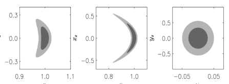
Figure 12: Two-dimensional probability distribution given by eqn. (30) with variables $x_{1},x_{2},$ for $\eta=1$ (left), $\eta=5$ (centre), and (right) the same distribution with transformed variables $y_{1}=x_{1}^{2}+x_{2}^{2}-1,y_{2}=x_{2}.$

Figure 13: Variation in inverse efficiency $1/E$ with step-size $\sigma_{T}/\sigma_{0}$, for the distributions shown in Fig.  12 with curvature parameters $\eta=1$ and $\eta=5$ (upper curves) as defined in the text. Parameter $x_{1}$ is dot-dashed, $x_{2}$ is dashed, compared to the transformed parameters $y_{i}$ (solid).

In the second example, the simply connected region of high probability has the shape of a thin crescent (shown in Fig. 12). A simple change of variable can in principle solve the problems described above. The pathology of this distribution can be characterized by the dimensionless parameter $\eta=\sigma^{2}_{\theta}/\sigma_{r},$ which gives the approximate number of standard deviations by which the region of highest probability is displaced from the two-dimensional mean. Any change of variable that renders the region convex (for example one which locally resembles polar coordinates) makes the underlying distribution sufficiently close to Gaussian in the new variable, so that the previously described methods are adequate. Here for example the new parameters $y_{1}=x_{1}^{2}+x_{2}^{2}-1,y_{2}=x_{2}$ transform the crescent to a bivariate Gaussian.

We investigate the effect of using the original coordinates on the efficiency of a chain sampled using the standard Gaussian trial distribution. We take two examples with $\eta=1$ and $\eta=5$, whose distributions are shown in Fig. 12, following the same procedure as described in section 5 to measure the efficiency as a function of the step-size. As the distributions are no longer symmetric we use ${\mn@boldsymbol{C}}_{T}=\sigma_{T}/\sigma_{0}{\mn@boldsymbol{C}},$ measuring a separate efficiency for each parameter. In Fig. 13 these results can be compared to the optimal efficiency for a Gaussian, obtainable using the transformed coordinates (solid line). For the mildly curved distribution with $\eta=1$ the efficiency is simply reduced by a factor $\sim 1.5$, but the optimal step-size is unchanged. The more extreme $\eta=5$ case shows markedly different behaviour however, with the less efficient $x_{1}$ parameter fifteen times slower than the optimal Gaussian case, for a step-size twice as big and a far lower acceptance rate, $f_{A}\sim 0.05$. The high curvature and long tails make it impossible to converge quickly using a Gaussian trial distribution, since the trial and underlying distributions overlap so badly. Low acceptance rates combined with diffusive steps result in highly correlated chains. In practice this slowdown is readily diagnosed using our spectral test while running the chain. Coupled with a tendency towards a very low acceptance rate for a naive optimal step-size $\sigma_{T}/\sigma_{0}\sim 2.4/\sqrt{D},$ this would be a clear indication of the need to reparametrize.

In high dimensions it is often difficult to identify an appropriate change of variables empirically, although Kosowsky, Milosavljevic & Jimenez (2002) and Jimenez et al. (2004) describe such a transformation of a set of simple-inflationary cosmological parameters into a set of nearly-orthogonal ‘physical’ parameters. In practice however, we have found the non-transformed cosmological parameters to be sufficiently well-behaved for flat cosmologies, achieving high efficiencies.

6.3 Bimodal or multi-peaked distributions

Failure of the spectral convergence test is most likely to occur for distributions having multiple narrow peaks of high probability connected by wide regions of low probability. While the length $N_{\rm single~{}peak}$ required to sample adequately the region around a single peak may be rather short, the length $N_{\rm tunnel}$ required to tunnel to other peaks may be substantially longer.

The simplest example is a symmetric bimodal distribution

$$p(x)={1\over 2}{1\over\sqrt{2\pi}}\left\{\exp\left[-{(x-a)^{2}\over 2}\right]+\exp\left[-{(x+a)^{2}\over 2}\right]\right\}$$ (31)

with variable peak position at $x=\pm a$. We wish to know if the spectral convergence test can fail for this model by indicating convergence before the full distribution is recovered. The behaviour of the chain will depend on both $a$ and the trial step-size $\sigma_{T}/\sigma_{0}$. We explore this dependency and its effect on the chain power spectrum by sampling from the distribution with variable peak separation $a$, using a fixed trial distribution width $\sigma_{T}$.

Figure 14: Behaviour of chains with fixed trial distribution sampling a bimodal distribution with peak positions $x=\pm 4$ (top 2 panels) $x=\pm 6$ (middle 4 panels) and $x=\pm 8$ (bottom panel). The chain output (left), recovered distributions (centre) and power spectra (right) are shown for various chain lengths $n$.

The observed behaviour, shown in Fig. 14, can be split roughly into three categories. For small peak separation $a$ the chain jumps between the two peaks frequently, converging toward both peaks simultaneously. The power spectrum only displays large-scale white-noise behaviour at late times when both peaks are fully sampled. The template fits the spectrum well at early and late times, shown in Fig. 14 (top two rows). If $a$ is increased sufficiently, then the chain may converge ‘locally’ on one of the peaks before it takes its first jump to the second peak, shown in the third row of Fig. 14 for $a=6$. Before it makes this jumps the chain would pass the spectral convergence test, but as soon as it swaps peaks an excess of power is produced on large scales (4th row). It now fails the convergence test, although the template does not provide a very good fit. After a much longer time (6th row) the chain will have sampled both peaks sufficiently to converge ‘globally’, recovering the correct distribution with peaks of equal height. The chain is no longer biased towards one of the peaks, so again the power becomes white-noise on large scales and the convergence test is passed. For large separation $a$ the chain can sample one peak without jumping to the second peak in any reasonable time. This is observed in Fig. 14 (bottom row) for $a=8$. For a length ten times longer than $N_{C}$ it does not jump, and we would falsely conclude that the distribution had only one peak. The same effect is seen if the peak separation is narrower (e.g. $a=6$) but the trial step-size is very small.

From these models we can conclude that if the chain visits a second peak even briefly, then it will show up as excess large-scale power in the power spectrum and the chain will not pass the convergence test until it has sampled both peaks sufficiently. This is useful since in high dimensions a jump might not be so obvious in the time-ordered chain output. If the peaks are very widely separated (or if an overly small step-size is being used) then the chain might not leave the first peak in a reasonable time. If there are just two peaks then multiple chains may be used to diagnose this problem, but for multiple disconnected peaks this could be insufficient, although this is an unlikely scenario for the case of cosmological parameters.

Figure 15: Variation in inverse efficiency $1/E$ with trial step-size $\sigma_{T}/\sigma_{0}$ and acceptance rate $f_{A}$ for a one-dimensional bimodal distribution with Gaussian peaks at $x=\pm a$ for $a=0$ (bottom), $2,4,6,8$ and $10$ (top).

Finally we investigate how the optimal scaling relations are altered if the distribution is bimodal, considering a range of peak separations from $a=2$ to $a=10$. Using the same methods described earlier, we find that the optimal step-sizes are similar to the Gaussian case, shown in Fig. 15, although slightly reduced to $\sigma_{T}/\sigma_{0}\sim 2.$ It is important to note that $\sigma_{0}$ applies here to the full distribution, not to a single peak. The optimal acceptance rate decreases as the peak separation increases, to $f_{A}\sim 0.1$ for $a=10.$ The inverse efficiency then gradually increases as the chain becomes more correlated as a consequence of steps occurring more infrequently. The unusual behaviour of the chain getting stuck indefinitely on one peak, seen in the final row of Fig.  14, occurs for step-sizes smaller than those considered here.

7 Sampling Method

This section outlines an explicit sampling procedure based on the methods and considerations presented in the previous sections. This is the procedure that we applied to extracting cosmological parameters from the CMB+LSS data.

1. An initial best guess is made for the covariance matrix of the underlying distribution ${\mn@boldsymbol{C}}_{1},$ which is used to fix the multivariate Gaussian trial distribution characterized by the covariance matrix ${\mn@boldsymbol{C}_{T}}_{1}$, chosen according to the rule

$${\mn@boldsymbol{C}_{T}}_{i}=(2.4^{2}/D){\mn@boldsymbol{C}}_{i}.$$ (32)

If possible, a starting point in the high likelihood region is chosen.

2. A short chain is sampled using ${\mn@boldsymbol{C}_{T}}_{1}$ to obtain a refined estimate for ${\mn@boldsymbol{C}}_{2},$ which in turn is used to update ${\mn@boldsymbol{C}_{T}}$ according to the same rule in eqn. 32 If this first chain started in a region of low likelihood, the first section (where $L/L_{max}\mathrel{\raise 1.29167pt\hbox{$<$}\mkern-14.0mu\lower 2.58334pt\hbox{$\sim$}}0.1$) is discarded before estimating ${\mn@boldsymbol{C}}_{2}.$ If the acceptance rate for this initial chain is very low (e.g. $\mathrel{\raise 1.29167pt\hbox{$<$}\mkern-14.0mu\lower 2.58334pt\hbox{$\sim$}}0.01$) or very high (e.g. $\mathrel{\raise 1.29167pt\hbox{$>$}\mkern-14.0mu\lower 2.58334pt\hbox{$\sim$}}0.9$), then this first chain does not provide a useful estimate of the covariance matrix and a new guess should be made for ${\mn@boldsymbol{C}}_{1}$.

3. A second chain is started with trial distribution ${\mn@boldsymbol{C}_{T}}_{2},$ starting where the previous chain finished. The process is iterated until further refinement would not lead to a sufficiently significant improvement in efficiency. The efficiency compared to ‘optimal’ can be judged using both the acceptance rate as an indicator, and the power spectrum test to give an estimate for $P_{0}.$ For real, approximately Gaussian distributions tested for dimension $D\mathrel{\raise 1.29167pt\hbox{$<$}\mkern-14.0mu\lower 2.58334pt\hbox{$\sim$}}8$ we have found that one update of the trial distribution to ${\mn@boldsymbol{C}_{T}}_{2}$ normally suffices to sample efficiently.

4. Only the final chain is used for the analysis, which is tested for convergence once $N>N_{c}$. The best-fit template for the power spectrum of each cosmological parameter is found, to give $P_{0}$, $\alpha$ and $k^{*}$. The test is passed if $k_{min}$ is in the regime $P(k)\propto k^{0},$ defined by the condition $j^{*}>20,$ and if the convergence ratio $r<0.01$ for each parameter. If the white noise-regime has been reached but $r>0.01$, an estimate can be made for how much longer the chain needs to run using $r\propto 1/N$.

6. Once the chain has converged, the histograms of the number densities are checked to insure sufficient points have been collected, and further sampling may be carried out if a characterisation of the wings of the distribution at high $\sigma$ are desired.

7. If a series of updates of the trial distribution fails to improve the efficiency or produce convergence, often signalled by a very low acceptance rate, it is likely that the distribution is highly non-Gaussian and reparametrization should be explored.

8 Application to CMB Parameter Estimation

We applied the above methods to estimating cosmological parameters using the CMB and LSS data and code as described in Bucher et al. (2004). Initially we consider a 7-dimensional pure adiabatic cosmological model defined by the parameters $\omega_{b},\omega_{d},\Omega_{\Lambda},n_{s},\tau,\beta,$ and an overall amplitude $A_{s}$. An appropriate trial distribution and high-likelihood starting point are easy to obtain given already-available results for this distribution in Spergel et al. (2003). After updating the trial distribution once, our second and final chain runs for 4000 steps with an acceptance rate of 26% before achieving convergence with white noise power at large scales and $r<0.01$ for all parameters. The values of the power spectrum template variables are given in Table 3 for the most and least efficient parameters. The underlying distribution is fairly close to Gaussian. We are able to sample very efficiently, achieving an inverse efficiency of $\approx 40$, compared to an optimal inverse efficiency of $\approx 25$ for $7$ dimensions. We continued running the chain to 9000 steps for improved statistics. Fig. 16 shows the time series of three of the seven parameters, their power spectra and best-fit curves and the recovered marginalized posterior distributions. The smoothed posterior distributions are obtained by fitting the logarithm of the binned number densities to a high order polynomial, as described in Tegmark et al. (2003).

Figure 16: MCMC chain for a pure adiabatic cosmological model, showing the chain output (left), power spectra (middle) and marginalized distributions (right) for three parameters of a 7-dimensional model, sampled with a chain of length $N=9000$.

We then extend the parameter space to 16 dimensions, including general isocurvature perturbations, requiring nine extra parameters to quantify the additional mode contributions. As described in Bucher et al. (2004), we include the CDM isocurvature mode and the neutrino density and velocity isocurvature modes, creating a $4\times 4$ symmetric mode matrix with the adiabatic mode and cross-correlations. Physically all the eigenvalues of this matrix must be non-negative. This constraint was imposed by assigning a zero likelihood to those trial steps violating it. With very little prior knowledge of this probability distribution and a higher cost of sampling non-optimally, the trial distribution was updated more times to improve the efficiency. The chain converged after $6\times 10^{4}$ steps, with $r_{i}<0.01$ for all parameters. In this chain 60% of steps violated the constraint, so that only $N_{models}=2.4\times 10^{4}$ actual cosmological models were evaluated. In Fig. 17 we show power spectra and the recovered distributions for four of the parameters, with the template variables given in Table 3. By taking an effective number of steps $N_{models}=24000$ we find an inverse efficiency of $1/E=240$ for the worst parameter. Since this distribution is non-Gaussian and of high dimension, it is not surprising that we do not achieve the optimal Gaussian inverse efficiency of $1/E=53.$

Figure 17: MCMC chain for a mixed adiabatic/isocurvature cosmological model. Power spectra (left) and marginalized distributions (right) for four parameters of the 16-dimensional model: the baryon density $\omega_{b}$, optical depth $\tau$ and relative power in two non-adiabatic modes, neutrino velocity ($NIV$) and correlated adiabatic/neutrino density isocurvature ($A,NID$).

	AD	AD	AD+ISO	AD+ISO
	best	worst	best	worst
$P_{0}=1/E$	$33$	$39$	$185$	$498$
$\alpha$	$1.8$	$1.8$	$1.8$	$1.8$
$j^{*}$	$90$	$77$	$92$	$37$

Table 3: Best-fit template variables for the power spectra of chains sampling cosmological parameters. All chains are normalized to have unit variance. The template parameters for the best (i.e., lowest $1/E$) and worst cosmological parameters are indicated for both the adiabatic models (AD) and the mixed adiabatic/isocurvature models (AD+ISO).

9 Discussion

We have shown how a spectral test based on an empirical fitting function can be used to diagnose reliably the convergence properties of a single long MCMC chain. Explicit criteria for convergence using this test were formulated and subsequently demonstrated to detect lack of convergence for a variety of underlying distributions. A procedure to optimize the covariance matrix for a Gaussian trial distribution was also explored.

The distributions for which our test did not successfully detect a lack of convergence were those with widely separated, narrow multiple peaks of high probability density. Although for such distributions no universally valid procedure exists for uncovering the presence of multiple peaks, a possible method is to run multiple chains starting from widely separated, randomly chosen points in the sample space. The Gelman & Rubin test provides an appropriate convergence diagnostic for multiple chains. The variance of the sample means of the several chains is compared to the estimated variance of the sampled distribution, obtained by averaging over the sample variance within each chain. In the case of multiple peaks or lack of convergence about a single peak, the variance of the sample means will be too high, failing to fall below a specified fraction of the within-chain sample variance.

The spectral test applied to single chains has the advantage of exploiting all the information relevant to estimating the sample mean variance. Rather than simply comparing a small number of parallel chains, the spectral test effectively divides the chain in $2j_{max}$ independent ways when all the $\hat{P}_{j}$ with $1\leq j\leq j_{max}$ are used to fit to the template.

We find that the spectral test and trial distributions optimized according to the procedure outlined above work well when applied to CMB parameter estimation. As described in detail above, a chain of length $N=4\times 10^{3}$ suffices to obtain $r\mathrel{\raise 1.29167pt\hbox{$<$}\mkern-14.0mu\lower 2.58334pt\hbox{$\sim$}}0.01$ (equivalent to a $10\%$ standard deviation for the sample means of the cosmological parameters) for an adiabatic cosmological model, although longer chains were actually employed to reduce shot noise error in the outer edge of the region of high probability. For the full adiabatic/isocurvature model, convergence was attained within $N=6\times 10^{4}$ steps, which involved calculating only $2.4\times 10^{4}$ distinct cosmological models due to large zero-likelihood regions. Neither model showed evidence of any of the pathologies explored in section 6. The chain performance attained may be compared to that expected from a Gaussian of the same dimension explored using a chain with an optimal trial distribution. Our efficiencies were lower by factors of approximately $1.6$ and $5$ for the two cases, respectively.

References

- (1) Christensen N., Meyer R., Knox L., Luey B., 2001, Class. Quant. Grav., 18, 2677
- (2) Best N. G., Cowles M. K.,Vines K., 1995, Technical Report, Medical Research Council Biostatistics Unit, Cambridge
- (3) Bucher M., Dunkley J., Ferreira P. G., Moodley K., Skordis C., 2004, PRL, in press (astro-ph/0401417)
- (4) Cowles M. K., Carlin B. P., 1996, J. Amer. Statist. Assoc, 91, 434
- (5) Doran M., Mueller C., 2003 (astro-ph/0311311)
- (6) Gelman A., Roberts G. O., Gilks W. R, 1996, in eds Bernardo J. M., Berger J. O., Dawid A., Smith A., Bayesian Statistics 5. 599, OUP
- (7) Gelman A., Rubin D. B., 1992, Statist. Sci., 7, 457
- (8) Geweke J., 1992, in eds Bernardo J. M., Berger J. O., Dawid A., Smith A., Bayesian Statistics 4 169, OUP
- (9) Gilks W. R., Richardson S., Spiegelhalter D. J., 1995, Markov Chain Monte Carlo in Practice. Chapman & Hall, London
- (10) Hanson K.M., Cunningham G. S., 1998, Proc. SPIE, 3338, 371
- (11) Heidelberger P., Welch P. D., 1981, Comm. ACM, 24, 233; 1985, Operations Research, 31, 1109
- (12) Hinshaw G. et al., 2003, ApJS, 148, 135
- (13) Jimenez R., Verde L., Peiris H., Kosowsky A., 2004, PRD, submitted (astro-ph/0404237)
- (14) Kogut A. et al., 2003, ApJS, 148, 161
- (15) Kosowsky A., Milosavljevic M., Jimenez R., 2002, PRD, 66, 063007
- (16) Knox L., Christensen N., Skordis C., 2001, ApJ, 563, L95
- (17) Lewis A., Bridle S., 2002, PRD, 66, 3511
- (18) Metropolis N., Rosenbluth A. W., Rosenbluth M. N., Teller A. H., 1953, J. Chem. Phys., 21, 1087
- (19) Neal R. M., 1993, Technical Report CRG-TR-93-1
- (20) Percival W. J. et al., 2001, MNRAS, 327, 1297
- (21) Raftery A.E., Lewis S. M., 1992, in eds Bernardo J. M., Berger J. O., Dawid A., Smith A., Bayesian Statistics 4 763, OUP
- (22) Slosar A., Hobson M. P., 2003, MNRAS, submitted (astro-ph/0307219)
- (23) Spergel D. et al., 2003, ApJ, 148, 213
- (24) Tegmark M. et al., 2003, PRD, in press (astro-ph/0310723)
- (25) Tegmark M. et al., 2003, ApJ, in press (astro-ph/0310725)
- (26) Verde L. et al., 2003, ApJS, 148, 195