Velocity Modification of Power Spectrum from Absorbing Medium

Abstract

Quantitative description of the statistics of intensity fluctuations within spectral line data cubes introduced in our earlier work is extended to the absorbing media. A possibility of extracting 3D velocity and density statistics from both integrated line intensity as well as from the individual channel maps is analyzed. We find that absorption enables the velocity effects to be seen even if the spectral line is integrated over frequencies. This regime that is frequently employed in observations is characterized by a non-trivial relation between the spectral index of velocities and the spectral index of intensity fluctuations. For instance when density is dominated by fluctuations at large scales, i.e. when correlations scale as $r^{-\gamma},~{}\gamma<0$, the intensity fluctuations exhibit a universal spectrum of fluctuations $\sim K^{-3}$ over a range of scales. When small scale fluctuations of density contain most of the energy, i.e. when correlations scale as $r^{-\gamma},~{}\gamma>0$, the resulting spectrum of the integrated lines depends on the scaling of the underlying density and scales as $K^{-3+\gamma}$. We show that if we take the spectral line slices that are sufficiently thin we recover our earlier results for thin slice data without absorption. As the result we extend the Velocity Channel Analysis (VCA) technique to optically thick lines enabling studies of turbulence in molecular clouds. In addition, the developed mathematical machinery enables a quantitative approach to solving other problems that involved statistical description of turbulence within emitting and absorbing gas.

1 Introduction

There is little doubt that interstellar medium is turbulent (see reviews by Armstrong, Spangler & Rickett 1995; Lazarian 1999a, Lazarian, Pogosyan & Esquivel 2002). Turbulence proved to be ubiquitous in molecular clouds (Dickman 1985), diffuse ionized (Cordes 1999) and neutral (Lazarian 1999b) media. Magneto-hydrodynamical (MHD) turbulence controls many essential astrophysical processes including star formation, transport and acceleration of cosmic rays, of heat and mass (see Schlickeiser 1999, Vazquez-Semadeni et al 2000, Narayan & Medvedev 2001, Wolfire et al. 2002, Cho et al. 2003, see recent reviews by Cho, Lazarian & Vishniac 2002, henceforth CLV02a, Elmegreen & Scalo 2004, Lazarian & Cho 2004). Unfortunately, we are still groping for the basic properties of interstellar turbulence. For instance, it is unclear whether turbulence in molecular clouds is a part of a global turbulent cascade or has its local origin.

Recent years were marked by a substantial progress in theoretical and numerical description of both incompressible and compressible MHD turbulent cascade (Goldreich & Shridhar 1995, Lithwick & Goldreich 2001, Cho & Lazarian 2002a, CLV02a, Cho & Lazarian 2003ab). It is encouraging that the measured statistics of electron density fluctuations (see Armstrong et al. 1995), synchrotron and polarization degree fluctuations (see Cho & Lazarian 2002b) are in rough correspondence with the theoretical expectations (see more discussion in Cho & Lazarian 2003b). Further testing requires better input data, and this makes the determination of actual power spectra of interstellar turbulence extremely important and meaningful. Indeed, it gives a chance to distinguish between different pictures of turbulence, e.g. shocks versus eddies picture, and put theoretical constructions developed for various interstellar processes, e.g. cosmic ray propagation (see Yan & Lazarian 2002), grain dynamics (Lazarian & Yan 2002, Yan & Lazarian 2003), stochastic reconnection (Lazarian & Vishniac 1999, Lazarian, Vishniac & Cho 2003) on a solid ground. Even within the picture of MHD cascade that is advocated by the simulations in Cho & Lazarian (2002) and which does not contain shocks, the distribution of energy between Alfven, slow and fast modes does depend on the turbulence driving. Therefore the spectra measured from observations can be used to constrain the driving. In addition, the particular features of the power spectrum, which are associated with energy injection and dissipation are important. Identification of such features and the spatial variations of their properties will shade light to the dynamics of interstellar gas and processes of star formation (see Lazarian & Cho 2003).

We should stress that while the statistics of density fluctuations can be only considered as an indirect way of testing turbulence, the spectral surveys contain the information about the direct measure, namely, the velocity statistics. This statistics is extremely valuable, provided that we can extract it from the observational data. As MHD turbulence is indeed an interdisciplinary subject, high resolution studies of interstellar turbulence can test contemporary ideas of MHD cascade. The implications of the improved understanding would affect description of wide range of astrophysical phenomena from solar flares to gamma ray bursts (see Lazarian et al. 2003).

Additional motivation for studying interstellar turbulence stems from the advances in direct numerical simulations of interstellar medium (see review by Vazquez-Semadeni et al 2000). Unlike MHD simulations focused on obtaining fundamental properties of turbulence (see CLV02a) those of interstellar medium attempt to include various aspects of interstellar physics. This usually limits the inertial range covered. However, testing of the numerical results against observations is becoming more interesting as numerical resolution increases. With other techniques of comparing numerics with observations having their problems (see review by Ostriker 2002, also Brunt et al. 2003) power spectra and second order correlation functions look as a promising tool for the future (see Lazarian 1995, Lazarian & Pogosyan 2000, henceforth LP00, Vestuto, Ostriker & Stone 2003). The potential of combining different techniques in order to get the properties of turbulence is also large.

Although in this paper we primarily refer to interstellar processes, the technique we discuss has a broader application. For instance, recent advances in X-ray astronomy have allowed to get information on turbulence in intracluster gas (see Inogamov & Sunyaev 2003, Sunyaev, Norman & Bryan 2003). The issues that researchers face there are similar to those dealt in interstellar turbulence studies.

To get insight into turbulent processes statistical approach is useful (see Monin & Yaglom 1976, Dickey 1995). So far, in astrophysical context the most tangible progress was achieved via scintillations and scattering technique (see Spangler 1999). Those measurements are limited to probing fluctuations of electron density on rather small scales, namely, $10^{8}$–$10^{15}$ cm. This research profited a lot from an adequate theoretical understanding of processes of scintillations and scattering (Goodman & Narayan 1985) and this made it very different from other branches of interstellar turbulence research. In comparison, formation of emission line profiles in turbulent media has not been properly described until very recently and it is natural that numerous attempts to study turbulence in diffuse interstellar medium, HII regions and molecular clouds using emission lines (see Munch 1958, O’Dell 1986, O’Dell & Castaneda 1987, Miesh & Bally 1994, reviews by Scalo 1987, Lazarian 1992) were only partially successful. This is very unfortunate as the line profiles contain unique information about turbulent velocity field. We reiterate that the studies of stochastic density provide only indirect insight into turbulence and cannot distinguish between active and fossil turbulence pictures.

Studies of the velocity field have been attempted at different times with velocity centroids (e.g. Munch 1958, Miesh, Bally & Scalo 1999, Miville-Deschenes, Levrier & Falgarone 2003). However, it has long been realized that the centroids are affected, in general, by both velocity and density fluctuations (see Stenholm 1989). An important criterion when centroids indeed reflect the velocity statistics was obtained in Lazarian & Esquivel (2003, henceforth LE03). LE03 showed that when the criterion is not satisfied the centroids are dominated by density. LE03 pointed out that the velocity centroids can be modified to extract the velocity contribution (LE03), but the resulting measures may be pretty noisy. As the result, velocity centroids taken alone may not be sufficiently robust and reliable technique. A recent study in Esquivel & Lazarian (2004) revealed that for Mach numbers larger than 2 or 3 the traditional velocity centroids fail. As Mach numbers as high as 10 are expected for molecular clouds the applicability of the traditional centroids to molecular clouds is highly questionable.

Principal Component Analysis (PCA) of the emission data (Heyer & Schloerb 1997, Brunt & Heyer 2002ab) has been suggested as a new way to study interstellar turbulence. However, recent testing showed that it provides statistics different from power spectra (Heyer, private communication, Brunt et al 2004). What sort of statistics we can obtain using the PCA requires a further study.

Wavelet analysis (see Gill & Henriksen 1990), Spectral Correlation Functions (see Rosolowsky et al. 1999, Padoan, Rosolowsky & Goodman 2001), genus analysis (see Lazarian, Pogosyan & Esquivel 2002) are other important statistical tools. They can provide statistics and insight complementary to power spectra (see review by Lazarian 1999a). Synergy of different techniques should provide the necessary insight into turbulence and enable the comparison of observational statistics with theoretical expectations (see Cho & Lazarian 2003a for a review).

Velocity statistics contributes to intensity variations observed in channel maps. Power-law spectra suggestive of underlying turbulence were obtained at different times by a number of researchers (see Kalberla & Mebold 1983, Green 1993). The problem that plagued those studies was inability to separate contributions due to velocity and density. Indeed, both velocity and density fluctuations affect the small-scale emissivity fluctuations observed at a given velocity. Therefore the separation of contributions to velocity and density requires a quantitative description of spectral line data cube statistics.

This problem was addressed in Lazarian & Pogosyan (2000, henthforth LP00), where the fluctuations of intensity in channel maps were related to the statistics of velocity and density. LP00 introduced a new statistical technique that was termed in Lazarian, Pogosyan & Esquivel (2002) Velocity Channel Analysis (henceforth VCA). Within VCA the separation of velocity and density contributions is obtained by changing the thickness of the analyzed slice of the Position-Position- Velocity (PPV) data cube. The theoretical description of the intensity statistics for both thick and thin velocity slices enabled LP00 to disentangle velocity and density contributions to intensity fluctuations in PPV cubes.

The VCA was successfully tested numerically in Lazarian et al. (2001) and Esquivel et al. (2003). Those tests employed the velocity and density obtained via simulations of compressible MHD turbulence to obtain synthetic maps, which were analyzed using VCA to recover underlying velocity statistics. Since then the VCA has been successfully applied to get velocity spectra of turbulence (see section 5).

The VCA in its existing form, however, does not account for absorption of radiation. LP00 argued that for the 21 cm emission data the effect of absorption is marginal in the direction of the galactic anti-center for which the technique was applied. However, the data in Dickey et al (2001) show substantial absorption in HI towards inner part of the Galaxy. Moreover, the absorption is definitely essential for other, e.g. CO transitions.

The purpose of this paper is to extend the earlier obtained theoretical description of the Doppler-shifted spectral line data cubes by including the treatment of absorption effects and thus to obtain a quantitative tool to study turbulence in various interstellar conditions, including molecular clouds. We introduce the 3D anisotropic statistics of fluctuations within PPV data cubes in section 2, describe effects absorption in section 3, provide the statistics for thin and thick slices in section 4, explain some of our findings in physical terms in section 5, discuss our results and their implications for observational data in section 6. The summary is provided in section 7. The lengthy derivations are collected in the appendixes which are an important part of the paper.

2 Statistics of Velocity and Density

2.1 Basics of Turbulence Statistics

Statistics in Real Space
In the presence of magnetic field MHD turbulence gets axisymmetric in the system of reference related to the local direction of magnetic field. In this system of reference magnetic fields can be easily mixed by turbulence in the direction perpendicular to magnetic fields. Those mixing motions generate wave-like perturbations propagating along magnetic field lines. As the kinetic energy decreases with the decrease of the scale, the weak mixing motions bend magnetic field lines less and less and the eddies get more and more elongated.

The Goldreich & Shridhar (1995) model of incompressible turbulence prescribes Kolmogorov scaling of mixing motions perpendicular to magnetic field lines (see a simplified discussion in CLV02a) and the elongation of the velocity fluctuations that increases as $l^{1/3}$. Further research in Lithwick & Goldreich (2001) and Cho & Lazarian (2002) has shown that the basic features of the Goldreich-Shridhar turbulence carry on for Alfvenic perturbations to the compressible regime.

Observations, however, are usually unable to identify the local orientation of magnetic field and deal with the magnetic field projection integrated over the line of sight. As the result the locally defined perpendicular and parallel directions are mixed together in the process of observations (see CLV02a). The fluctuations with more power dominate the signal for both the direction of the averaged ${\bf B}$ and perpendicular to it. There is some residual anisotropy, but this anisotropy is scale-independent and is determined by the rate of the meandering of the large scale field. In other words, from the observational point of view the spectra of intensity fluctuations obtained from the Goldreich & Shridhar turbulence and the isotropic turbulence are similar. Observations in Green (1993) and numerical studies in Esquivel et al. (2003) support this picture.

The facts above allow for a substantial simplification of the turbulence description, namely, they permit us to use standard isotropic statistics (Monin & Yaglom 1976). Obtaining this statistics would correspond to obtaining the scaling of density and velocity fluctuations perpendicular to magnetic field lines.

Statistically isotropic in $xyz$-space density field $\rho({\bf x})$ has the correlation function

$$\xi(r)=\xi({\bf r})=\langle\rho({\bf x})\rho({\bf x}+{\bf r})\rangle~{}~{}~{}.$$ (1)

We shall also use the correlation function of density fluctuations $\delta\rho=\rho-\langle\rho\rangle$

$$\tilde{\xi}(r)=\langle\delta\rho({\bf x})\delta\rho({\bf x}+{\bf r})\rangle=\xi(r)-\langle\rho\rangle^{2}~{}.$$ (2)

The structure function

$$d(r)=\langle(\rho({\bf x}+{\bf r})-\rho({\bf x}))^{2}\rangle~{}~{}~{},$$ (3)

is another way of describing turbulence. Here $\tilde{d}(r)$ for fluctuations coincides with $d(r)$.

Statistical descriptors of fluctuations can often be assumed to have power-law dependence on scale $\propto r^{-\gamma}$. If the correlation is dominated by large scales, the structure functions are used and $\gamma<0$, while for small scale dominated statistics the correlation functions are usually used and $\gamma>0$. We show in Appendix A that the two cases in the asymptotic regime of small $r$ can be treated very similarly. Therefore we will frequently refer to correlation functions having in mind both $\gamma>0$ and $\gamma<0$.

An isotropic velocity field ${\bf u}({\bf x})$ is fully described by the structure tensor $\langle\Delta u_{i}\Delta u_{j}\rangle$, which can be expressed via longitudinal $D_{LL}$ and transverse $D_{NN}$ components (Monin & Yaglom 1972)

$$\langle\Delta u_{i}\Delta u_{j}\rangle=\left(D_{LL}(r)-D_{NN}(r)\right){r_{i}r_{j}\over r^{2}}+D_{NN}(r)\delta_{ik}~{}~{}~{},$$ (4)

where $\delta_{ik}$ equals 1 for $i=k$ and zero otherwise. We define z-projection of the velocity structure function as

$$D_{z}({\bf r})\equiv\langle\Delta u_{i}\Delta u_{j}\rangle\hat{z}_{i}\hat{z}_{j}=D_{NN}(r)+[D_{LL}(r)-D_{NN}(r)]\cos^{2}\theta~{},~{}~{}~{}\cos\theta\equiv{\bf\hat{r}\cdot\hat{z}}$$ (5)

which for the power-law velocity gives

$$D_{z}({\bf r})=Cr^{m}[1+\frac{m}{2}(1-\cos^{2}\theta)]~{}~{}~{},$$ (6)

if we assume that the velocity is solenoidal. For this paper it is only important that $D_{z}\sim Cr^{m}$. A discussion of the shallow and steep spectra of density as well as of the velocity statistics within finite size clouds is given in Appendix A.

Spectra and Correlation Functions
Spectra and correlation/structure functions are two complementary ways of describing turbulence. Given an N-dimensional correlation function $\xi_{N}(\bf r)$ one can obtain the spectrum

$$P({\bf k})=\int d^{N}{\bf r}e^{i{\bf k}{\bf r}}\xi_{N}(\bf r)~{}~{}~{},$$ (7)

where the integration is performed in the $N$-dimensional space.

In LP00 the Fourier space statistics, namely, spectra were widely used with the correlation functions playing an auxiliary role. In the present paper we deal with absorption defined in real space. Therefore we use real space statistics, namely, correlation and structure functions functions. It is obvious from eq. (7) that for power-law correlation function (CF), i.e. $\xi_{N}\sim r^{-\gamma}$ the spectral index is also a power-law, i.e. $P\sim k^{n}$, where $n=-N+\gamma$. In other words,

$$({spectral~{}index})=(-{dimensions~{}of~{}space}-{CF~{}index})$$ (8)

In Kolmogorov turbulence passive scalar density correlations scale as $r^{2/3}$, which corresponds to $\gamma=-2/3$ in our notations. Thus the Kolmogorov spectrum index is $-11/3$. In turbulence literature $E(k)=4\pi k^{2}P(k)$ is usually used. In this notation the Kolmogorov spectrum is $E(k)\sim k^{-5/3}$, and thus, the Kolmogorov law is often referred to as $-5/3$ law.

2.2 Statistics in PPV

One does not observe the gas distribution in the real space galactic coordinates xyz where the 3D vector ${\bf x}$ is defined. Rather, intensity of the emission in a given spectral line is defined in Position-Position-Velocity (PPV) cubes towards some direction on the sky and at a given line-of-sight velocity $v$. In the plane parallel approximation the direction on the sky is identified with xy plane where the 2D spatial vector ${\bf X}$ is defined, so that the coordinates of PPV cubes available through observations are $({\bf X},v)$. The relation between the real space and PPV descriptions is defined by a map $({\bf X},z)\to({\bf X},v)$.

The central object for our study is a turbulent cloud in PPV coordinates. The statistical properties of the PPV density $\rho_{s}({\bf X},v)$ depend on the density of gas in real galactic coordinates, but also on velocity distribution of gas particles. Henthforth we use the subscript $s$ to distinguish the quantities in $({\bf X},v)$ coordinates from those $({\bf X},z)$ coordinates. We shall always assume 2D statistical homogeneity and isotropy of $\rho_{s}({\bf X},v)$ in ${\bf X}$-direction over the image of a cloud. However, homogeneity along the velocity direction can only be assumed after additional considerations, if at all. Naturally, there is no symmetry between $v$ and ${\bf X}$.

We shall use the following notation for statistical descriptors of the density in PPV space: the mean density is $\bar{\rho}_{s}(v_{1})=\langle\rho_{s}({\bf X}_{1},v_{1})\rangle$, and the correlation functions of the density and, closely related, the density fluctuations $\delta\rho_{s}({\bf X}_{1},v_{1})=\rho_{s}({\bf X}_{1},v_{1})-\bar{\rho}_{s}(v_{1})$ are

$$\xi_{s}(R,v_{1},v_{2}) \equiv \langle\rho_{s}({\bf X}_{1},v_{1})\rho_{s}({\bf X}_{2},v_{2})\rangle$$ (9)

$$\tilde{\xi}_{s}(R,v_{1},v_{2}) \equiv \langle\delta\rho_{s}({\bf X}_{1},v_{1})\delta\rho_{s}({\bf X}_{2},v_{2})\rangle=\xi(R,v_{1},v_{2})-\bar{\rho}_{s}(v_{1})\bar{\rho}_{s}(v_{2})~{}.$$ (10)

Here we have maintained notation which highlights the symmetries of the statistics. Homogeneity and isotropy in Position-Position coordinates ${\bf X}$ lead the mean density to depend only on velocity while the correlation function depends only on the magnitude of separation between two sky directions $R=|{\bf R}|=|{\bf X}_{1}-{\bf X_{2}}|$. Dependence on the velocity is retained for the time being in the general form.

For PPV statistics it is more convenient to use the structure functions

$$d_{s}(R,v_{1},v_{2}) = \langle\left[\rho_{s}({\bf X}_{1},v_{1})-\rho_{s}({\bf X}_{2},v_{2})\right]^{2}\rangle$$ (11)

$$\tilde{d}_{s}(R,v_{1},v_{2}) = \langle\left[\delta\rho_{s}({\bf X}_{1},v_{1})-\delta\rho_{s}({\bf X}_{2},v_{2})\right]^{2}\rangle=d_{s}(R,v_{1},v_{2})-\left[\bar{\rho}_{s}(v_{1})-\bar{\rho}_{s}(v_{2})\right]^{2}$$ (12)

Let us derive the two-point correlation function in PPV space without using the power spectrum formalism employed in LP00. The line-of-sight component of velocity $v$ at the position ${\bf x}$ is a sum of the regular gas flow (e.g., due to galactic rotation) $v_{gal}({\bf x})$, the turbulent velocity $u({\bf x})$ and the residual component due to thermal motions. This residual thermal velocity $v-v_{gal}({\bf x})-u({\bf x})$ has a Maxwellian distribution

$$\phi_{v}({\bf x}){\mathrm{d}}v=\frac{1}{(2\pi\beta)^{1/2}}\exp\left[-\frac{(v-v_{gal}({\bf x})-u({\bf x}))^{2}}{2\beta}\right]{\mathrm{d}}v~{}~{}~{},$$ (13)

where $\beta=\kappa_{B}T/m$, $m$ being the mass of atoms. The temperature $T$ can, in general, vary from point to point.

The density of the gas in the PPV space $\rho_{s}({\bf X},v)$ can then be written as

$$\rho_{s}({\bf X},v){\mathrm{d}{\bf X}d}v=\left[\int_{0}^{S}{\mathrm{d}}z\;\rho({\bf x})\phi_{v}({\bf x})\right]{\mathrm{d}{\bf X}d}v~{}~{}~{},$$ (14)

where $\rho({\bf x})$ is the (random) density of gas in real space. This expression just counts the number of atoms along the line-of-sight that have z-component of velocity in the interval $[v,v+dv]$. The limits of integration are defined by the spatial extend $S$ of the emitting gas distribution.

To compute the correlation function $\xi_{s}$ we disregard the effect of correlations between density and velocity fluctuations:

$$\langle\rho_{s}({\bf X}_{1},v_{1})\rho_{s}({\bf X}_{2},v_{2})\rangle = \int_{0}^{S}dz_{1}\int_{0}^{S}dz_{2}\;\langle\rho({\bf x}_{1})\rho({\bf x}_{2})\rangle\;\langle\phi_{v1}({\bf x}_{1})\phi_{v2}({\bf x}_{2})\rangle~{}~{}~{},$$ (15)

$$\langle\rho_{s}({\bf X},v)\rangle = \int_{0}^{S}dz\langle\rho({\bf x})\rangle\langle\phi_{v}({\bf x})\rangle$$ (16)

The brackets $\langle\cdots\rangle$ in eq. (16) denote statistical averaging over realizations of the random density $\rho({\bf x})$ and the turbulent velocity $u({\bf x})$ of gas. In particular, for the density we can write $\langle\rho({\bf x})\rangle=\bar{\rho}$ and $\langle\rho({\bf x}_{1})\rho({\bf x}_{2})\rangle=\xi(\bf r)$, without any assumptions on density statistics. For the Gaussian velocity field $u$, described by structure functions given by eq. (4), the statistical average of the Maxwell functionals (13) is given in Appendix B (see (B8) (B), (B4)).

The general expression for the correlation function given in the Appendix B (see eq.(B3) can be simplified if one neglects the edge effects associated with the wings of spectral lines (see derivation of eq. (B7)). In this case we have

$$\xi_{s}({\bf R},v)\sim\frac{1}{2\pi(CS)^{m/2}}\int_{-S}^{S}{\mathrm{d}}z\int_{|z|/2}^{S-|z|/2}{\mathrm{d}}z_{+}\;\xi({\bf r})\;[D_{z}({\bf r})+2\beta]^{-1/2}\exp\left[-\frac{(v-v_{gal})^{2}}{2(D_{z}({\bf r})+2\beta)}\right],$$ (17)

where eq. (A2) was used to write the prefactor explicitly. For a homogeneous statistics all correlation functions depend only on the separation between points. Here and further on we use variables without indexes to denote separation, as in ${\bf R=X_{1}-X_{2}}$, $z=z_{1}-z_{2}$, $v=v_{1}-v_{2}$ and $v_{gal}=v_{gal,1}-v_{gal,2}$. Variables with an index ’+’ denote the average of two arguments $z_{+}=(z_{1}+z_{2})/2$, etc. Dependence on these last quantities appears only if statistical homogeneity is broken, e.g. by a finite spatial extend of the gas distribution.

In the absence of the turbulent and thermal motions, $D_{z},\beta\to 0$, the kernel in eq. (17) reduces to the delta-function $\delta(v-v_{gal})$, and for monotonic $v_{gal}(z)$ one can fully recover the line of sight position of an emitting atom from its velocity. In a general case, while thermal broadening just smothers fluctuations out, the effect of the turbulent velocity fluctuations is scale dependent and leads to a change of the correlation function slope.

Equation (17) allows for an arbitrary form of the regular flow $v_{gal}$. A variable regular flow produces a complex map from galactic to velocity space by itself. Two tractable cases are when the regular flow is of a simple linear form, or the one when it is possible to attribute all motions to turbulence, thus setting $v_{gal}=0$. In LP00 we have considered the case of linearized shear flow $v_{gal}=f^{-1}z$ due to Galactic rotation:

$$\xi_{s}({\bf R},v)\sim\int_{-\infty}^{\infty}{\mathrm{d}}z\;\xi({\bf r})\;[D_{z}({\bf r})+2\beta]^{-1/2}\exp\left[-\frac{(v-f^{-1}z)^{2}}{2(D_{z}({\bf r})+2\beta)}\right],$$ (18)

where we have omitted an unimportant dimensional prefactor (see eq. (B) for the explicit form of the prefactor). Galactic shear introduces a natural scale $\lambda={\left[f^{2}C\right]}^{1\over 2-m}$, at which the velocity dispersion $\sim C\lambda^{m}$ becomes equal to the squared difference of the regular velocities determined by Galactic rotation (i.e. $f^{-2}\lambda^{2}$). Asymptotics obtained in LP00 correspond to the scales $l$ which are much smaller than $\lambda$. Although at these scales galactic rotational velocity is much larger than the turbulent one, it’s gradient is much smaller than the turbulent one. It is because of that the LP00 results in the presence of Galactic rotation and without it coincide. The regime when the small scales turbulent shear exceeds the regular one is natural. Indeed, flows with high Reynolds number produce turbulence with shear larger that that of the original flow. This is true, for instance, for Couette flows in the presence of the moderately strong magnetic field (Velikhov 1959, Chandrasechar 1962, Balbus & Hawley 1991). The corresponding criterion on the magnetic field is usually satisfied in the interstellar medium.

If gas is confined in an isolated cloud of size $S$ and the galactic shear over this scale is neglected we get

$$\xi_{s}({\bf R},v)\sim\int_{-S}^{S}{\mathrm{d}}z(1-\frac{|z|}{2S})\;\frac{\xi({\bf r})}{[D_{z}({\bf r})+2\beta]^{1/2}}\exp\left[-\frac{v^{2}}{2(D_{z}({\bf r})+2\beta)}\right],$$ (19)

where again somewhat ugly prefactor entering eq. (B) is omitted. Turbulent effects remain important up to the scale of the cloud $S$ at which turbulent structure function saturates at the value $\sim(CS^{m})^{1/2}$. The cloud size $S$ now plays the role of the scale $\lambda$. This observation allows to translate the LP00 results mostly written for Galactic HI with rotation curve mapping to a case of an individual cloud. Rigorous calculations provided in LP00 prove that for scales much smaller than $S$ one can use the results obtained for infinite medium in the presence of shear and substitute $\lambda$ for $S$.

When the amplitude of fluctuations grows with separation, one should use structure functions in PPV. The transfer from one type of statistics to another is similar to that discussed in Appendix A.

Important feature of the PPV space is that $\rho_{s}({\bf X},v)$ exhibits fluctuations even if the flow is incompressible and no density fluctuations are present. Indeed, when one substitutes the expanded expression (A4) $\xi({\bf r})=\bar{\rho}^{2}+\bar{\rho}^{2}(r_{0}/r)^{\gamma}$ into eqs (17-19), both terms will give rise to non-trivial contributions to $\tilde{\xi}_{s}({\bf R},v)$. We shall therefore split the result correspondingly

$$\tilde{\xi}_{s}({\bf R},v) = \tilde{\xi}_{v}({\bf R},v)+\tilde{\xi}_{\rho}({\bf R},v),$$

$$\tilde{d}_{s}({\bf R},v) = \tilde{d}_{v}({\bf R},v)+\tilde{d}_{\rho}({\bf R},v).$$ (20)

with the $v$-term describing pure velocity effects, while the $\rho$-term arising from the actual real space density inhomogeneities that are modified by velocity mapping. To simplify the notation we have dropped index $s$ from the right-hand-side quantities, since this split is only meaningful in PPV space. In Appendix C we discuss asymptotic small-R scalings of different contributions to PPV structure and correlation functions.

3 Turbulent Statistics and Radiative Transfer

We start with the standard equation of radiative transfer (Spitzer 1978)

$$dI_{\nu}=-g_{\nu}I_{\nu}ds+j_{\nu}ds~{}~{}~{}.$$ (21)

In the case of self-adsorbing emission in spectral lines that is proportional to first power of density:

$$g_{\nu}=\alpha(z)\rho(z)\phi_{v}(z)~{}~{}~{},$$ (22)

$$j_{\nu}=\epsilon\rho(z)\phi_{v}(z)~{}~{}~{},$$ (23)

where $\phi_{v}(z)$ is given by (13).

A solution of this equation if no external illumination is present is

$$I_{v}=\epsilon\int^{S}_{0}dz\rho(z)\phi_{v}(z)\exp\left(-\int_{0}^{z}\alpha(z^{\prime})\rho(z^{\prime})\phi_{v}(z^{\prime})dz^{\prime}\right)~{}~{}~{}.$$ (24)

To integrate (24) we shall assume that $\alpha$ is constant. This constancy is the essence of the Sobolev approximation that was found to be useful in many astrophysical applications. In this approximation we can use an integration variable

$$Y_{v}(z)=\int_{0}^{z}\rho(z^{\prime})\phi_{v}(z^{\prime})dz^{\prime}~{}~{},$$ (25)

which value at $x=S$ coincides with the density in PPV coordinates, $Y_{v}(S)=\rho_{s}({\bf X},v)$, and $Y_{v}(0)=0$, to integrate eq.(24)

$$I_{v}({\bf X})=\epsilon\int^{\rho_{s}}_{0}dY_{v}{\mathrm{e}}^{-\alpha Y_{v}}=\frac{\epsilon}{\alpha}\left[1-{\mathrm{e}}^{-\alpha\rho_{s}({\bf X},v)}\right]~{}~{}~{}.$$ (26)

In the case of vanishing absorption, the intensity is given by the linear term in the expansion of the exponent in eq. (26)

$$I_{v}({\bf X})=\epsilon\rho_{s}({\bf X},v)~{}~{}.$$ (27)

and reflects the PPV density of the emitters. If, however, the absorption is strong, the intensity of the emission is saturated at the value $\epsilon/\alpha$ wherever $\rho_{s}({\bf X},v)\gg 1/\alpha$. Identification of the low contrast residual fluctuations may be difficult in practice.

The approximate expression given by eq. (26) can be used to find the statistics of the expected emissivity fluctuations. First of all, the mean profile of the line is given by

$$\langle I_{v}({\bf X})\rangle=\frac{\epsilon}{\alpha}\left[1-\langle{\mathrm{e}}^{-\alpha\rho_{s}({\bf X},v)}\rangle\right]~{}~{}~{}.$$ (28)

Our main goal is to calculate the structure function of the observed emissivity

$${\cal D}({\bf R})\equiv\left\langle\left(\int I_{v}({\bf X}_{1})W_{v}dv-\int I_{v}({\bf X}_{2})W_{v}dv\right)^{2}\right\rangle,~{}~{}~{}{\bf R}={\bf X}_{1}-{\bf X}_{2}~{}~{}~{}.$$ (29)

Here the window function $W_{v}$ describes how the integration over velocities is performed. When $W_{v}\equiv 1$ the integration is being performed over the whole line as it is a frequent case for CO turbulence studies (see Falgarone et al. 1998, Stutzki et al. 1998) while measurements in velocity slices of PPV data cube (channel maps) correspond to $W_{v}$ strongly peaked at a particular velocity. Within the VCA technique by varying the width of velocity channels one can obtain statistics of turbulent velocities and density inhomogeneities of emitting medium. Note, that the minimal width of the velocity channel is determined by the resolution of an instrument.

Using elementary identities to transfer from averaging over 2D intensities to averaging the underlying 3D fluctuations (see Lazarian 1995), in the limit when the absorption can be neglected we rewrite the expression (29) in the form

$${\cal D}({\bf R})=\epsilon^{2}\int\,dv_{1}W(v_{1})\int\,dv_{2}W(v_{2})\left[d_{s}({\bf R},v_{1},v_{2})-d_{s}(0,v_{1},v_{2})\right]$$ (30)

where homogeneity in physical directions is assumed. For infinite emitting medium homogeneous turbulence produces a homogeneous image in the velocity space. For finite emitting cloud the PPV image is approximately homogeneous over velocity separations much less than the Doppler linewidth. Notably, the combination in brackets does not depend on the mean Doppler broadened profile of the spectral line, $d_{s}({\bf R},v_{1},v_{2})-d_{s}(0,v_{1},v_{2})=\tilde{d}_{s}({\bf R},v_{1},v_{2})-\tilde{d}_{s}(0,v_{1},v_{2})$. Thus, it is sufficient to assume that in the $v$-direction fluctuations of $\rho_{s}$ are homogeneous. In this case,

$${\cal D}({\bf R})=\epsilon^{2}\int~{}dvW(v)\left[d_{s}({\bf R},v)-d_{s}(0,v)\right]$$ (31)

with $W(v)=\int dv_{+}W(v_{+}-v)W(v_{+}+v)$. The formula (31) together with Appendix B can be taken as a starting point to reproduce the results in LP00 using structure functions rather than spectra (compare with LP00). This is demonstrated in Appendix D.

Substitution of the expression (26) into (29) gives

$${\cal D}({\bf R}) = \frac{\epsilon^{2}}{\alpha^{2}}\int\,dv_{1}W(v_{1})\int\,dv_{2}W(v_{2})\times$$ (32)

$$\times \langle e^{-\alpha(\rho_{11}+\rho_{12})}+e^{-\alpha(\rho_{22}+\rho_{21})}-e^{-\alpha(\rho_{21}+\rho_{12})}-e^{-\alpha(\rho_{11}+\rho_{22})}\rangle$$

where we have used a shorthand notation $\rho({\bf X}_{i},v_{j})=\rho_{ij}$. Homogeneity in spatial directions dictates that after averaging the first term is equal to the second one and the third is equal to the fourth (e.g. for the density itself $\langle\rho_{11}+\rho_{12}\rangle=\langle\rho_{22}+\rho_{21}\rangle$ and $\langle\rho_{12}+\rho_{21}\rangle=\langle\rho_{11}+\rho_{12}\rangle$).

We shall now derive an approximate expression for ${\cal D}({\bf R})$, applicable for small separations $R$. Let us rewrite eq. (32) as

$${\cal D}({\bf R}) = \frac{\epsilon^{2}}{\alpha^{2}}\int\,dv_{1}W(v_{1})\int\,dv_{2}W(v_{2})\times$$ (33)

$$\times \langle e^{-\alpha(\rho_{11}+\rho_{12})}\left[1+e^{-\alpha(\rho_{22}+\rho_{21}-\rho_{11}-\rho_{12})}-e^{-\alpha(\rho_{21}-\rho_{11})}-e^{-\alpha(\rho_{22}-\rho_{12})}\right]\rangle~{}~{}.$$

It is easy to see that the term in brackets depends only on the differences in density taken between two lines of sight at the same velocity, i.e. $\rho_{11}-\rho_{21}$ and $\rho_{22}-\rho_{12}$. The point of rearranging the terms in this way is that for small separations $R$ these differences are small, so we can retain only the leading order in the power series expansion for the corresponding exponentials

$${\cal D}({\bf R})\sim\epsilon^{2}\int\,dv_{1}W(v_{1})\int\,dv_{2}W(v_{2})\;\langle e^{-\alpha(\rho_{11}+\rho_{12})}\left[\left(\rho_{11}-\rho_{21}\right)\left(\rho_{12}-\rho_{22}\right)\right]\rangle~{}~{}.$$ (34)

The structure of the resulting expression is as follows. The term in brackets is similar to the integrand in eq. (30) (indeed, $\langle\left(\rho_{11}-\rho_{21}\right)\left(\rho_{12}-\rho_{22}\right)\rangle=d_{s}({\bf R},v_{1},v_{2})-d_{s}(0,v_{1},v_{2})$ ) while the effect of the absorption is manifested in the exponential term which depends on the density distribution in velocity direction along the line of sight. As we see, the series expansion we have performed at small separation $R$ is indeed an expansion that assumes $\alpha^{2}\left[d_{s}({\bf R},v_{1},v_{2})-d_{s}(0,v_{1},v_{2})\right]$ to be small. Similar expansion is then applicable for any combination of structure functions that vanishes at $R=0$ and this opens a way of dealing with non-Gaussian statistics.

Although there is a cross-correlation between the two terms in the integrand and statistical averaging cannot, in a general case, be factorized, the correction for cross-correlation is of a higher order of smallness than the leading term. This can be seen by expanding the remaining exponential term in power series. We can illustrate this statement by specifying Gaussian statistical distribution for $\rho_{s}$ and performing explicit averaging which then gives

$${\cal D}({\bf R})\sim\epsilon^{2}\int\,dv_{1}W(v_{1})\int\,dv_{2}W(v_{2})e^{\frac{1}{2}\alpha^{2}\langle(\rho_{11}+\rho_{12})^{2}\rangle}\left[d_{s}({\bf R},v_{1},v_{2})-d_{s}(0,v_{1},v_{2})+\alpha^{2}d_{12}\right]$$ (35)

The cross-correlation combination $d_{12}$ is vanishing as $R\to 0$ and $\alpha^{2}d_{12}$ is small, as expected. For non-Gaussian statistics the irreducible higher order correlations appear. However it is suggestive that these correlations provide vanishing contribution for $R\rightarrow 0$. Without providing a formal derivation for the general case, we propose that eq. (34) can be rewritten as

$${\cal D}({\bf R})\sim\epsilon^{2}\int\,dv_{1}W(v_{1})\int\,dv_{2}W(v_{2})\langle e^{-\alpha(\rho_{11}+\rho_{12})}\rangle\left[d_{s}({\bf R},v_{1},v_{2})-d_{s}(0,v_{1},v_{2})\right]~{}~{}.$$ (36)

or when approximation of homogeneity in velocity direction is warranted

$${\cal D}({\bf R})\sim\epsilon^{2}\int\,dv_{1}W(v_{1})\int\,dv_{2}W(v_{2})\langle e^{-\alpha(\rho_{11}+\rho_{12})}\rangle\left[d_{s}({\bf R},v)-d_{s}(0,v)\right]~{}.$$ (37)

Expressions (36) and (37) show that for sufficiently small $R$ the structure functions of intensity differ from the earlier studied case by the window function determined by the absorption $W_{absorption}=\langle e^{-\alpha(\rho_{11}+\rho_{12})}\rangle$. Two important conclusions directly follow from this observation. First, it is clear that if the window function determined by data slicing is much narrower than that given by the absorption we get results indistinguishable from the earlier studied case of no absorption. Second, in the case of integration over the whole line of sight, the results will be different from the earlier studied case because the window function is not equal to unity any more. The criterion when the absorption is not important for velocity studies is straightforward. Expression (37) transfers into (31) when $W_{absorption}$ is of the order of unity over the range of scales studied.

4 Scaling Regimes of the Emissivity Statistics

In this section we shall study emissivity statistics in the regimes when it exhibits power-law scaling. Such behavior is possible at the small scales where the effect of the absorption is limited $\alpha^{2}\left[d_{s}({\bf R},v_{1},v_{2})-d_{s}(0,v_{1},v_{2})\right]<1$ and eq. (37) provides a good approximation. We shall also restrict our consideration to the scales smaller than the cloud size $R/S\ll 1$ so that inhomogeneous boundary effects can be neglected.

4.1 Integrated Lines

The presence in eq. (37) of the window function determined by absorption, i.e. $\langle e^{-\alpha(\rho_{11}+\rho_{12})}\rangle$, changes substantially results compared to the case of no absorption discussed in LP00. Indeed, the integration over the whole spectral line in the latter case removes the dependence of intensity statistics on velocity. The window function determined by absorption defines to what extend the integration over velocities is performed.

Let us estimate the form of the window assuming Gaussian statistics and homogeneity of the density fluctuations $\delta\rho_{s}=\rho_{s}-\langle\rho_{s}\rangle$. Then (see eq. (E3))

$$W_{absorption}=e^{-\alpha\langle\rho_{s}({\bf X_{1}},v_{1})\rangle}e^{-\alpha\langle\rho_{s}({\bf X_{1}},v_{2})\rangle}e^{\alpha^{2}\langle\delta\rho_{s}^{2}({\bf X_{1}},v_{1})\rangle}e^{\alpha^{2}\langle\delta\rho_{s}^{2}({\bf X_{1}},v_{2})\rangle}e^{-\frac{\alpha^{2}}{2}{\tilde{d}}_{s}(0,v)}~{}~{}~{}~{}.$$ (38)

For homogeneous statistics the variance of the fluctuations does not depend on velocity thus the corresponding factors are constant and affect only the normalization of the result. However, their presence reveals limitations of the Gaussian approximation when the absorption is large. Indeed, a similar term appears in the mean line profile eq. (28) computed for Gaussian $\rho_{s}$, namely, $\langle I({\bf X},v_{1})\rangle=\frac{\epsilon}{\alpha}\left[1-\exp(-\alpha\langle\rho_{s}({\bf X_{1}},v_{1})\rangle+\frac{\alpha^{2}}{2}\langle\delta\rho_{s}^{2}({\bf X_{1}},v_{1})\rangle)\right]$. Clearly the answer is unphysical when $\alpha>2\langle\rho_{s}({\bf X_{1}},v_{1})\rangle/\langle\delta\rho_{s}^{2}({\bf X_{1}},v_{1})\rangle$. The problem arises because the Gaussian fluctuations do not obey the constraint that the density $\rho_{s}$ is positive. Therefore for high absorption, negative density excursions, however rare, dominate the result. In view of this, we select in eq. (38) the factors which describe the variable part of the mean intensity profile, and write them in non-expanded form

$$W_{absorption}=\langle e^{-\alpha\rho_{s}({\bf X_{1}},v_{1})}\rangle\langle e^{-\alpha\rho_{s}({\bf X_{1}},v_{2})}\rangle e^{\frac{\alpha^{2}}{2}\langle\delta\rho_{s}^{2}({\bf X_{1}},v_{1})+\delta\rho_{s}^{2}({\bf X_{1}},v_{2})\rangle}e^{-\frac{\alpha^{2}}{2}{\tilde{d}}_{s}(0,v)}$$ (39)

This approximate formula does not suffer from the defect we have mentioned. The residual dependence on $\delta\rho_{s}$ variance can be traced to the real effect of increase of intensity contrast between two points if absorption is present. However, this factor is constant in our treatment and we shall normalize it out. We summarize our considerations in the formula

$${\cal D}({\bf R})\propto\int\,dv\;\tilde{W}(v)\;e^{-\frac{\alpha^{2}}{2}{\tilde{d}}_{s}(0,v)}\;\left[d_{s}({\bf R},v)-d_{s}(0,v)\right]~{},$$ (40)

where

$$\tilde{W}(v)\equiv\int{\mathrm{d}}v_{+}W(v_{1})W(v_{2})\langle e^{-\alpha\rho_{s}({\bf X_{1}},v_{1})}\rangle\langle e^{-\alpha\rho_{s}({\bf X_{1}},v_{2})}\rangle~{}~{}~{}~{}~{}.$$ (41)

The most important effect induced by absorption is an additional exponential down-weighting in the projection of the contribution from the points with large velocity separation $v$ in a manner which itself depends on the turbulence statistics. For subsonic turbulence where the velocity variance is dominated by the thermal dispersion and is not scale dependent, the effect of absorption in our approximation amounts to a constant and for statistics is equivalent to zero absorption and zero turbulent velocity case. However, one should still check whether the linearization of the kernel holds at the scales under study for a given absorption value.

The most important qualitative characteristic of the window is its width, which for absorption we shall define as velocity $v_{ab}$ at which

$$\alpha^{2}\tilde{d}_{s}(0,v_{ab})=1~{}~{}~{}~{}~{}~{}~{}.$$ (42)

In terms of the velocity-density decomposition of the PPV structure function, the product of the two windows arise $\sim e^{-\alpha^{2}\tilde{d}_{v}(0,v)/2}e^{-\alpha^{2}\tilde{d}_{\rho}(0,v)/2}$. Both factors act simultaneously but the one with the smallest width determines the gross effect. Asymptotic analysis of $\tilde{d}_{s}(0,v)$ in Appendix C gives for the absorption window widths

$$v_{ab}/D_{z}(S)^{1/2} \approx \left(\alpha\bar{\rho}\right)^{\frac{2m}{m-2(1-\gamma)}},~{}~{}~{}~{}~{}~{}m>2/3\;(1-\gamma)$$ (43)

$$v_{ab}/D_{z}(S)^{1/2} \approx \left(\alpha\bar{\rho}\right)^{-1}~{}~{}~{}~{}~{}~{}~{},~{}~{}~{}~{}~{}~{}m<2/3\;(1-\gamma)$$ (44)

where we have omitted numerical coefficients of order unity and estimated the mean density in PPV space as

$$\langle\rho_{s}\rangle=\bar{\rho}S/D_{z}(S)^{1/2}~{}~{}.$$ (45)

Absorption effects become negligible if $v_{ab}/D_{z}(S)^{1/2}\gg 1$.

Effect of Velocity Fluctuations
Let us consider first the $\delta\rho_{s}$ fluctuations that arise from velocity fluctuations only. Indeed, even if the underlying density is constant, random velocities do produce caustics that were shown in LP00 to be very important for the analysis.

In Figure 1 we plot the correspondent kernel $\left[d_{v}({\bf R},v)-d_{v}(0,v)\right]$ as a function of $v$ for a fixed sample value of $R$ and, simultaneously, the window function $e^{-\frac{\alpha^{2}}{2}{\tilde{d}}_{s}(0,v)}$ for the range of absorption amount characterized by $\alpha\bar{\rho}_{s}$. The kernel is highly peaked at the zero velocity separation $v=0$, has region of negative values, and approaches zero at large $v$. The window is unity for zero absorption but also peaks at $v=0$ as absorption increases.

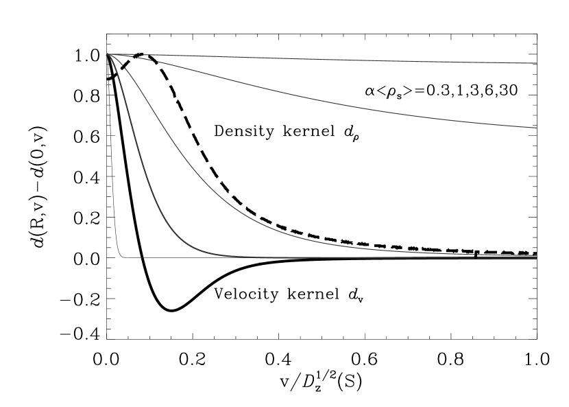
Figure 1: The velocity kernel $d_{v}(R,v)-d_{v}(0,v)$ (thick solid line) and the density kernel $d_{\rho}(R,v)-d_{\rho}(0,v)$ (dotted line) for $R/S=0.01$ and $m=2/3$ as a function of the line of sight velocity separation $v/D_{z}^{1/2}(S)$ normalized over velocity dispersion. The thin solid lines correspond to the window function $\exp(-\alpha^{2}{\tilde{d}}_{s}(0,v)/2)$ and are drawn for the values $\alpha\langle\rho_{s}\rangle$ from $0.3$ to $30$ (from top to bottom). For the displayed value of $R$, the linearized treatment of the kernels is applicable up to $\alpha\langle\rho_{s}\rangle\sim\sqrt{2}(R/S)^{(m-2)/4}\approx 6$, the corresponding line is highlighted.

Integration of the velocity kernel over the whole line in the absence of absorption and $W(v)=1$ gives zero, in concordance with the expectation of canceling all the velocity effects. In the presence of high absorption one might hope that down-weighting all nonzero $v$ contribution will act as an effective thin slice reproducing thin slice power-law asymptotics of $D(R)$, which is achieved when the width of the slice becomes small compared to rms velocity at the scale of the study $R$ (LP00). However we are restricted by the fact that our linearized approximation (34) is valid only when absorption is moderate $\alpha^{2}d_{s}({\bf R},0)<1$, while higher absorption (or larger scales at fixed $\alpha$) will induce nonlinear modifications of the result. Thus we find thin slice scaling is never realized for $m\geq 2/3$. Instead, the new universal intermediate power-law scaling is exhibited for moderate absorption. Dependence of the 2D structure function on the underlying velocity index $m$ is lost in this regime For $m<2/3$ there is a range of scales when absorption can modify the scaling to that of the thin slice in which case sensitivity to $m$ is present.

Analytical estimates can provide some insight into the expected behavior of ${\cal D}_{v}({\bf R})$ after integration as $R\to 0$. The value of the kernel at the peak, $d_{v}({\bf R},0)$ is given by the asymptotic expression (C4) (see also LP00 for asymptotics of the correlation functions in the velocity space),

$$d_{v}(R,0)\sim\left|\frac{\sqrt{\pi}\;\Gamma(m/4-1/2)}{\Gamma(m/4)}\right|R^{1-m/2}~{}~{}~{},$$ (46)

where we are more interested in the $R$ dependence of the expression than in the numerical prefactor. Incidently, this gives a criterion on the validity of the linear expansion of the velocity kernel. With dimensional quantities restored the condition

$$\alpha^{2}\langle\rho_{s}\rangle^{2}<\left|\frac{\Gamma(m/4)}{\sqrt{\pi}\Gamma(m/4-1/2)}\right|\left(\frac{S}{R}\right)^{1-m/2}$$ (47)

sets the scale range where our treatment is applicable.

Let us first consider the case $m\geq 2/3$. With the width of absorption induced window given by eq. (43), the condition (47) requires $v_{ab}^{2}\gtrsim D_{z}(S)(R/S)^{m}$, i.e velocity cutoff exceeds rms turbulent velocity at scale $R$ and thus is insufficient to reproduce thin slice which require opposite relation to be true (see LP00).

This is, however, sufficient to suppress the negative large $v$ tail in which case the dominant contribution to the integral scales as the height of the kernel peak times its width. The scaling of the width of the kernel peak with $R$ can be readily obtained from the following consideration: If we integrate the kernel over $v$ choosing fixed integration range $dV$ but varying $R$ from large values to the small, then the projected result will scale with $R$ according to thin slice asymptotics while $D_{z}(R)^{1/2}>dV$. The change to the thick slice behavior takes place when the condition is reversed. But formally in the thin slice regime the integral is determined by the zero-lag peak behavior only, while in the thick slice integration encompasses most of the kernel. Therefore $dV=D_{z}(R)^{1/2}$, where $D_{z}(R)$ is the $z$ projection of the correlation tensor of velocity (see eq.(5), represents the required estimate of the width of the kernel. This scaling is valid both for the zero crossing point of the velocity kernel and the width of the density kernel that we consider later.

The total scaling of the 2D emissivity structure function is thus ${\cal D}_{v}(R)\sim d_{v}(R,0)dV\propto R^{1-m/2}R^{m/2}\propto R$, with dependence on $m$ canceled out. The corresponding 2D spectra scales as $K^{-3}$.

Numerical integration using eq. (35) confirms that indeed the velocity statistics exhibit a new intermediate asymptotic regime, which is characterized by a universal spectral index of $-3$. In Fig. 2 we show structure functions of intensity for two different indexes $m=2/3$ and $m=1$. The range for the universal asymptotics is clearly seen.

Figure 2: The structure function of intensity for $m=2/3$ (right panel) and $m=1$ (left panel) for a set of absorption coefficients $\alpha\langle\rho_{s}\rangle=0.2,0.36,0.7,2.5$ (from top to bottom). We use the general non-linear expressions from Appendix E, but plot the curves only up to $R$ when linearized theory is still accurate. At the intermediate scales $R$ the structure function tends to the universal regime $\sim R$ which does not depend on the particular index $m$. The upper dashed line corresponds to the thick slice asymptotics for the velocity (spectral index $-3-m/2$) and the lower dotted line correspond to the universal index $-3$ that does not depend on $m$.

Fig. 2 also shows that for very small $R$ the structure function grows faster than $R$, which entails spectra steeper than $K^{-3}$. Indeed, for sufficiently small $R$ the $\exp(\alpha^{2}{\tilde{d}}_{v}(0,v))$ window does not cut out even the distant region where the kernel gets negative in which case we expect to see the thick slice asymptotics $\sim R^{1+m/2}$ (i.e $K^{-3-m/2}$ for the spectrum, see LP00) in accordance with our numerical calculations. Thermal effects (not included in numerical experiment) at scales where turbulence is subsonic $D_{z}(R)<\beta$ lead to even faster fall-off of the structure function at small $R$ and indeed make any coherent scaling of turbulent velocity hard to observe in emissivity statistics at that scales.

For $m<2/3$, on the other hand, absorption may lead to thin slice scaling $\propto R^{1-m/2}$ for some intermediate range of scales before $R$ is so large as to cause nonlinear deviations. Indeed, in this case $\left(\alpha\bar{\rho}\right)\approx v_{ab}/D_{z}(S)^{1/2}$ and condition (47) can be rearranged to read $D_{z}(R)/v_{ab}^{2}(R/S)^{1-3m/2}<1$ which can be satisfied even for relatively high absorption $v_{ab}^{2}/D_{z}(R)>1$ correspondent to thin slice velocity cutoff. For a given absorption parametrized by $v_{ab}$ we summarize the behaviour at the different scales

$$\begin{array}[]{lll}\mathrm{Scale~{}Range}&\mathrm{Intensity~{}Scaling}&\mathrm{Regime}\\ \hline\cr\\ R/S<(\beta/D_{z}(S))^{1/m}&\mathrm{velocity~{}effects~{}erased}&(\mathrm{subsonic~{}regime})\\ R/S\ll\left(\frac{v_{ab}^{2}}{D_{z}(S)}\right)^{1/m}&{\cal D}(R)\propto R^{1+m/2}&(thick~{}\mathrm{slice})\\ R/S<\left(\frac{v_{ab}^{2}}{D_{z}(S)}\right)^{1/m}&{\cal D}(R)\propto R^{1}&(\mathrm{intermediate~{}scaling})\\ \left(\frac{v_{ab}^{2}}{D_{z}(S)}\right)^{1/m}<R/S<\left(\frac{v_{ab}^{2}}{D_{z}(S)}\right)^{2/(2-m)}&{\cal D}(R)\propto R^{1-m/2}&(thin~{}\mathrm{slice})\\ \left(\frac{v_{ab}^{2}}{D_{z}(S)}\right)^{2/(2-m)}<R/S&\mathrm{not~{}a~{}power~{}law}&(\mathrm{strong~{}absorption~{}regime})\end{array}$$

Table 1: Scalings of structure functions of intensity fluctuations arising from velocity fluctuations for the power-law underlying 3D velocity statistics. In the strong absorption regime ${\cal D}$ does not follow a simple power-law. Thin slice regime does not exist for $m>2/3$. $D_{z}(S)$ is given by eq.(5).

in the Table 1. All four scaling regimes are present for $m<2/3$ although how pronounced is actually thin slice scaling (1) depends on the extend of the scale range $(v_{ab}^{2}/D_{z}(S))^{1/m}$ — $(v_{ab}^{2}/D_{z}(S))^{2/2-m}$, which grows with absorption strength if $m<2/3$. This interval does not exist for $m\geq 2/3$. We note that the two-dimensional emissivity statistics of integrated lines ${\cal D}_{v}(R)$ restore $m$ sensitivity for $m<2/3$ where the line-of-sight statistics $\tilde{d}_{v}(0,v)$ is saturated at $\propto v^{2}$. The latter behavior is not surprising. Indeed, structure functions $\tilde{d}_{v}(0,v)$ cannot grow faster than $v^{2}$ and this explains the saturation. However, the information along the line of sight is not lost. The analysis of the spectra of fluctuations along the velocity coordinate performed in LP00 confirms this.

Effect of Density Fluctuations
Density fluctuations modify the statistics of emissivity. Mathematically the density fluctuations are imprinted on the $\xi_{\rho}$ part of the 3D correlation function. This correlation function depends both on the statistics of density and velocity. As we discussed earlier, density correlations may be short-wave or long-wave dominated. Within power-law model for over-density statistics they are described, respectively, by correlation $\tilde{\xi}(r)=\bar{\rho}^{2}(r_{0}/r)^{\gamma}$ or structure $\tilde{d}(r)=\bar{\rho}^{2}(r_{0}/r)^{\gamma}$ functions, where $\gamma$ is positive in the former and negative in the latter case (see Appendix A). The amplitude of the density effect is encoded in the correlation scale $r_{0}$ which has a meaning of the scale at which density inhomogeneities have an amplitude equal the mean density of the gas (i.e. $\delta\rho\sim\bar{\rho}$ for $\gamma>0$ or $\rho_{1}-\rho_{2}\sim\bar{\rho}$ for $\gamma<0$). This gives rise to the amplitude factor $(r_{0}/S)^{\gamma}$ in the asymptotic expressions of Appendix C (e.g. eq. (C5)).

Contribution from density to PPV statistics combines linearly with the pure velocity term and an important question of which term dominates arises. Note, that both terms contribute to the absorption window at the same time in non-linear fashion.

Table 2 summarizes at which scales the density inhomogeneity contribution dominates velocity effects in PPV space.

$$\begin{array}[]{lllc}\mathrm{Condition}&\mathrm{Case}~{}\gamma<0&\mathrm{Case}~{}\gamma>0&\mathrm{Eqns}\\ \hline\cr\\ \tilde{d}_{\rho}(R,0)>\tilde{d}_{v}(R,0):&R>r_{0}&R<r_{0}&(\ref{AppC:eq_dvR},\ref{AppC:eq_drhoR})\\ \\ \tilde{d}_{\rho}(0,v)>\tilde{d}_{v}(0,v):&&&\\ m\geq\mathrm{max}\left[\frac{2}{3},\frac{2}{3}(1-\gamma)\right]&v^{2}>D_{z}(S)(r_{0}/S)^{m}&v^{2}<D_{z}(S)(r_{0}/S)^{m}&(\ref{AppCeq:d_vVfg23},\ref{AppCeq:d_rhoVf1})\\ \frac{2}{3}<m<\frac{2}{3}(1-\gamma)&v^{2}>D_{z}(S)(r_{0}/S)^{-\frac{2/3\gamma m}{m-2/3}}&\mathrm{not~{}applicable}&(\ref{AppCeq:d_vVfg23},\ref{AppCeq:d_rhoVf2})\\ \frac{2}{3}(1-\gamma)<m<\frac{2}{3}&\mathrm{not~{}applicable}&v^{2}<D_{z}(S)(r_{0}/S)^{\frac{2/3\gamma m}{m-2/3(1-\gamma)}}&(\ref{AppCeq:d_vVfl23},\ref{AppCeq:d_rhoVf1})\\ m\leq\mathrm{min}\left[\frac{2}{3},\frac{2}{3}(1-\gamma)\right]&r_{0}/S<1&r_{0}/S>1&(\ref{AppCeq:d_vVfl23},\ref{AppCeq:d_rhoVf2})\end{array}$$

Table 2: Range of the scales where the impact of density inhomogeneities to the PPV statistics exceeds the velocity contribution. For steep spectra $\gamma<0$, we need $r_{0}<S$ for density effects to be seen. This is feasible in a model where high amplitude density inhomogeneities are saturated at scales $r_{c}<S$. For the validity of the asymptotic scaling used, $R\ll S~{}(\mathrm{or}~{}r_{c})$ is required. When $\tilde{d}_{\rho}(0,v)>\tilde{d}_{v}(0,v)$ the window function is determined by $\tilde{d}_{\rho}(0,v)$ (see eq. (42)). In addition, the window function is determined by density fluctuations for subsonic velocities.

For steep spectra, the density contribution dominates large scales, above characteristic scale determined by $r_{0}$, For shallow spectra it is dominant at small scales. Density inhomogeneities also dominate observed statistics at small scales where velocity is subsonic.

What are the reasonable values for $r_{0}$ ? We argue that the amplitude of density perturbations of the scale of the cloud itself should not significantly exceed the mean density, otherwise the applicability of the notion of a cloud is suspect. For a shallow spectrum $\gamma>0$ this means $r_{0}<S$. For a steep spectrum $\gamma<0$, $r_{0}>S$ is likely, if a power-law distribution of fluctuation amplitudes extends all the way to the cloud scale $S$. In both cases $(r_{0}/S)^{\gamma}<1$.

An immediate conclusion from Table 2 is that for steep spectra $\gamma<0$ density terms are expected to always be subdominant, since within a cloud $R\leq S<r_{0}$. However we must stress that this relies on an assumption that the turbulent density scaling extends all the way to the cloud size $S$, in which case high value of $d(S)$ will indicate large inhomogeneities of the size of the whole cloud. But if the density structure function saturates at smaller separation $r_{c}<S$, e.g. as $\tilde{d}(r)=\tilde{d}(\infty)r^{-\gamma}/(r^{-\gamma}+r_{c}^{-\gamma})$, we may encounter a high amplitude $\tilde{d}(\infty)\gg\bar{\rho}^{2}$ without density at the scale of the cloud being significantly perturbed, since all inhomogeneities are restricted to smaller scales. As seen from the expansion $\tilde{d}(r)\sim\tilde{d}(\infty)(r/r_{c})^{-\gamma},~{}~{}r<r_{c}$, the effective correlation scale in this case is $r_{0}=r_{c}\times[\bar{\rho}^{2}/\tilde{d}(\infty)]^{-1/\gamma}<r_{c}$ and in the range of scales $r_{0}<R<r_{c}$ one will observe the density effects. The physical picture, leading to such situation, is to have strong energy injection at scale smaller than a cloud size, with turbulent cascade establishing steep spectrum to smaller scales, while having energy sources only weakly correlated at larger scales.

The Table 2 shows that for a shallow spectrum the density term is important for PPV statistical descriptors in both $R$ and $v$ direction at small scales $R<r_{0}$ and $v^{2}<D_{z}(r_{0})$ (for $m\geq 2/3$).

The marked effect of absorption on intensity fluctuations in integrated lines is that the density contribution cannot always be recovered by increasing the slice thickness, as it is the case of no or small absorption. On the contrary, we are able to observe the density impact on the emissivity only in restricted scale range. The reason for this is that for a wide range of scales above the thermal dispersion scale the velocity term is not suppressed in the presence of the absorption even when we integrate over the whole line.

We shall now discuss the how the density contribution scales, depending on separation $R$ and conditions on $\gamma$ and $m$. Whether density term will dominate the overall PPV statistics depends on the amplitude of density inhomogeneities given by $r_{0}$ according to Table 2. Our results are summarized below in Table 3.

Scaling estimations for density are obtained in a similar way to the case of pure velocity term in the previous section. The main ingredients are density kernel and absorption windows, exemplified in Figure 1. The complication is that the absorption window is determined by $d_{s}(0,v)$, with contributions from both velocity and density giving rise to two multiplicative windows (see equation (42)). The one with the smallest width of the two is the most important one. We shall explicitly note when the details of the absorption window are important.

The peak of the density kernel now scales as $R^{1-\gamma-m/2}$ (see equation C5) while its width is $dV\sim D_{z}(R)^{1/2}$, as we discussed before. Integrating over the whole line in the absence of absorption gives an estimate ${\cal D}(R)\propto R^{1-\gamma-m/2}R^{m/2}\sim R^{1-\gamma}$ (this refers to a correlation, rather than to a structure function of emissivity if $\gamma>1$). which is exactly the thick slice regime of LP00. If absorption is not too strong, $v_{ab}>D_{z}(R)^{1/2}$, it will not affect this result. This is different from pure velocity term, since the velocity term exactly vanishes when integrated over the whole velocity range in the absence of absorption, and small absorption leads to qualitatively new intermediate ”universal” scaling.

The condition of weak absorption in the presence of density, that replaces the one in (47), is given by

$$\alpha^{2}\langle\rho_{s}\rangle^{2}<\left|\frac{\Gamma(\gamma/2+m/4)}{\sqrt{\pi}\Gamma(\gamma/2+m/4-1/2)}\right|\left(\frac{S}{R}\right)^{1-\gamma-m/2}$$ (48)

Using (43,44) to express absorption via $v_{ab}$, we find familiar constraints when absorption effects are not strongly non-linear

$$v_{ab}^{2} > D_{z}(S)(R/S)^{m}\sim D_{z}(R),~{}~{}~{}~{}~{}~{}~{}~{}~{}~{}~{}~{}~{}~{}~{}~{}~{}~{}m>2/3\;(1-\gamma)$$ (49)

$$v_{ab}^{2} > D_{z}(S)(R/S)^{1-\gamma-m/2}~{}~{}~{}~{}~{},~{}~{}~{}~{}~{}~{}~{}~{}~{}~{}~{}~{}~{}~{}~{}~{}~{}~{}m<2/3\;(1-\gamma)$$ (50)

$$\begin{array}[]{lll}\mathrm{Scale~{}Range}&\mathrm{Intensity~{}Scaling}&\mathrm{Regime}\\ \hline\cr\\ R/S<(\beta/D_{z}(S))^{1/m}&{\cal D}(R)\propto R^{1-\gamma}&(\mathrm{subsonic})\\ R/S<\left(\frac{v_{ab}^{2}}{D_{z}(S)}\right)^{1/m}&{\cal D}(R)\propto R^{1-\gamma}&(\mathrm{thick~{}\mathrm{slice}})\\ \left(\frac{v_{ab}^{2}}{D_{z}(S)}\right)^{1/m}<R/S<\left(\frac{v_{ab}^{2}}{D_{z}(S)}\right)^{\frac{2}{2-2\gamma-m}}&{\cal D}(R)\propto R^{1-\gamma-m/2}&(thin~{}\mathrm{slice})\\ \left(\frac{v_{ab}^{2}}{D_{z}(S)}\right)^{2/(2-m)}<R/S&\mathrm{not~{}a~{}power~{}law}&(\mathrm{strong~{}absorption})\end{array}$$

Table 3: Scalings of structure functions of intensity fluctuations arising from density inhomogeneities for the power-law underlying 3D velocity statistics. Thin slice behaviour require $\gamma<1-3m/2$. In the strong absorption regime ${\cal D}$ does not follow a simple power-law.

The first case, $m>2/3(1-\gamma)$ is applicable for the most interesting values of $m$ if the density spectrum is shallow, $\gamma>0$. Here, linearity and thick slice conditions coincide and one cannot achieve thin slice regime before the absorption effects become nonlinear.

The second case, $m<2/3(1-\gamma)$ has wide range of applicability for steep spectra $\gamma<0$. Here linearity condition is less stringent and in the range of scales $(v_{ab}^{2}/D_{z}(r_{c}))^{1/m}<R/r_{c}<(v_{ab}^{2}/D_{z}(r_{c}))^{1/1-\gamma-m/2}$ absorption effects modify the emissivity scaling towards the thin slope $R^{1-\gamma-m/2}$, while nonlinear effects come into play only at larger scales. .

To summarize: For shallow spectra one expects line-integrated statistics for density perturbations to follow thick slice scaling until absorptions effects become too strong. Density terms are visible in the overall emissivity statistics at $R<r_{0}$. For steep spectra, density contribution may exhibit, in addition to thick slice behaviour at small scales, the thin slice scaling at intermediate scales. However, density contribution can be dominant in emissivity statistics only when $R>r_{0}$, which require high amplitude density inhomogeneities saturated at scales smaller than a cloud size.

Table 3 and Fig. 3 illustrate how the statistics of emissivity changes with the change of the spectral index of density and velocity.

Figure 3: Left panel: The structure function of intensity for Kolmogorov density and Kolmogorov velocity. Right panel: The structure function of intensity for shallow density $\gamma=1/2$ Kolmogorov velocity $m=2/3$. Absorption parameter for the lines shown varies in the range $\alpha\langle\rho_{s}\rangle(r_{0}/S)^{\gamma/2}=0.1$ (top) to $1$ (bottom). Scaling solutions for both cases are given in heavier line and labeled. The calculations are done using unexpanded formula given by eq. (E4). The non-linear effects get important as $R$ increases.

Can we ever observe density fluctuations in the absorbing gas outside the ranges set by correlation scales, for example when turbulent velocities are small ? While one decreases the amplitude of supersonic turbulence the absorption effects increase due to atoms concentrating at similar velocities which is expressed by PPV density $\bar{\rho}_{s}\approx\bar{\rho}S/\sqrt{D_{z}(S)+2\beta}$ growth, making recovering turbulence scaling more difficult. However velocity effects disappear as turbulence becomes subsonic at all scales $D_{z}(S)\ll\beta$. The power law index of density inhomogeneities can then be obtained over the range of scales if $\alpha\bar{\rho}S/\sqrt{\beta}\ll 1$. Under similar conditions we can see density fluctuations at small scales $r<r_{\rm thermal}$, where the turbulence is subsonic even if it is supersonic at large scales. The scale $r_{\rm thermal}$ can be determined as $D_{z}(r_{\rm thermal})=\beta$.

It may look somewhat counterintuitive that even in the absence of velocity we never see a thin skin of the cloud exhibiting 2D spatial slice of density fluctuations. As absorption is proportional to density in our model, the optical depth changes with the change of density. As the result the emission fluctuations are not dominated by the atoms within the thin skin depth from the cloud surface. The origin of the effect can be traced to original equations of radiative transfer (see eq. (26)). For instance, in the absence of velocity effects $\rho_{s}$ is proportional to the integral over the whole line of sight (see eq. (25)).

4.2 Thin Velocity Slices of Spectral Line Data

Within the VCA technique introduced in LP00 the change of the spectral index of emission fluctuations with the thickness of the channel maps was employed to separate the contributions from density and velocity. In particular, to see the thin slice scaling that reflects the statistics of turbulent velocities, the effective window of the velocity slice should be narrower than the turbulent velocity dispersion at the scale of the study.

The thermal broadening (i.e. $\beta$ factor in the previous section) of the line can be considered as a convolution with the window $W_{slice}$ describing the channel slicing adopted in the data analysis. The LP00 study showed that adopting the slice thickness less than the thermal width $\delta V<\beta$ does not provide new information about turbulence. In our discussion we shall treat thermal effects as adding (in quadrature) the minimum width to the data slice, symbolically ${\delta V}^{2}+\beta$

Absorption results in appearance of the second window function $W_{absorption}$. Two cases can take place.

If $v_{ab}^{2}<{\delta V^{2}}+\beta$ the regime is not different from that discussed in the earlier subsection. Indeed, it is the absorption that limits the integration and the results of integration over the slice thickness and over the whole emission line should be similar. According to previous discussion, absorption smoothing reveals the underlying velocity statistics only for $m<2/3$. Since the thermal broadening is given by the properties of the media under study and therefore is fixed, we get the following picture. If absorption is strong $v_{ab}^{2}<\beta$ making slices thinner will not provide any additional information about turbulence. This is the case when the velocity information recovered using the VCA is limited if any.

In case $v_{ab}^{2}>\beta$ one can get information about turbulence by making the slice thinner, i.e. decreasing $\delta V$ to ${\delta V}^{2}<v_{ab}^{2}-\beta$. Choosing the thickness of the velocity slice to ensure that $v_{ab}^{2}>{\delta V}^{2}+\beta$ we formally return to the regime very similar to that considered in LP00. Indeed, if the window function defined by the absorption is unimportant we return to the case mathematically similar to that in LP00. Naturally our results obtained in this regime are identical to those in LP00. Fig. 4 shows what is happening when we choose thin slicing for self absorbing data. It is easy to see that in doing so we get back to the regime of thin slices discussed in LP00.

As the result we can extend the VCA for self-absorbing clouds and provide observers with a following recipe:
1. If the integrated line emissivity shows a universal spectrum with $n=-3$, this testify that the density statistics is steep. In this case thin slice regime would provide one with a spectrum, which power-law index is $-3+m/2$.
2. If the integrated line emissivity shows a spectrum which is shallower than $-3$, this index should be identified with the power-law index $n$ of the underlying 3D density field. The thin slice regime in this case provides the index $n+m/2$.

It is clear that in the case of shallow density the VCA recovers both 3D velocity and density spectra, while in the case of steep density the VCA would normally recover just velocity spectral index. Potentially, one may attempt to remove the universal statistics in this case, but this may be very challenging in practical terms. It is also evident that for subsonic turbulence thin slice regime is not attainable.

5 Accomplishments and Qualitative Understanding of Results

Let us start with an explanation what has been done so far in different parts of the present paper. We started with introducing radiative transfer in §3 and obtaining general expressions for the statistics of intensity in the presence of the radiative transfer. We showed that absorption plays the role of an additional window function in those expressions. Then in §4 we discuss the two limiting and observationally important cases. One is related to the way how most present day observations of fluctuations are performed, namely, through measuring fluctuations of the integrated intensity. In this situation we show that the information about the underlying statistics in most cases is lost. We show, however, that the information can be recovered if fluctuations in velocity slices are analyzed. These are two major results of the paper.

A good deal of the paper and most of the Appendixes deal with the statistics of the fluctuations without absorption. This was necessary because the earlier machinery was formulated in terms of power spectra, while the transformation from the PPV power spectra to correlation functions happen to be not trivial. In terms of our earlier work, this not only provides an independent check of our results in LP00, but provides a very important extension of the technique. For instance, we obtain the predictions for the statistics of fluctuations along the velocity direction. These fluctuations can be studied using instruments with good spectral resolution even if the spatial resolution of the instruments is poor.

With the mathematical machinery in the paper being sufficiently involved, the issue of qualitative understanding of our results is of a particular interest. Especially this is important for our results that may look somewhat counterintuitive.

Consider first the formulae for thin slices. The spectrum of intensity in a thin slice gets shallower as the underlying velocity get steeper. To understand this effect consider turbulence in incompressible optically thin media. The intensity of emission in a slice of data is proportional to the number of atoms per the velocity interval given by the thickness of the data slice. Thin slice means that the velocity dispersion at the scale of study is larger than the thickness of a slice. The increase of the velocity dispersion at a particular scales means that less and less energy is being emitted within the velocity interval that defines the slice. As the result the image of the eddy gets fainter. In other words, the larger is the dispersion at the scale of the study the less intensity is registered at this scale within the thin slice of spectral data. This means that steep velocity spectra that correspond to the flow with more energy at large scales should produce intensity distribution within thin slice for which the more brightness will be at small scales. This is exactly what our formulae predict for thin slices (see also LP00).

The result above gets obvious when one recalls that the largest intensities within thin slices are expected from the regions that are the least perturbed by velocities. If density variations are also present they modify the result. When the amplitude of density perturbation becomes larger than the mean density, both the statistics of density and velocity are imprinted in thin slices. For small scale asymptotics that we are mostly interested in the paper, this happens, however, only when the density spectrum is shallow, i.e. dominated by fluctuations at small scales.

Understanding of the results for integrated spectral line in the presence of absorption is a bit more involved. Again, it is advisable to consider incompressible flows first. If no absorption present the integrated spectral line images are not affected by velocity fluctuations. Indeed, the velocity field just redistributes atoms along the line of sight and this redistribution cannot affect the total intensity in the absence of absorption.

If absorption is present, the fact that velocity redistributes atoms along the line of sight causes fluctuations of the integrated intensity. Two effects, however, are present simultaneously as the velocity field at a particular scale spreads atoms in PPV space. It is easy to see that the most absorption is expected is when the atoms have the same velocities. Therefore velocity dispersion provided by turbulence decrease the absorption and therefore increases the signal. However, the decrease of the optical thickness makes the media to behave more like its optically thin counterpart, in which the velocity fluctuations are averaged out. In other words, while the mean level of intensity increases as the result of turbulence, the contrast of the fluctuations caused by the velocity fluctuations decreases. The range of the universal asymptotics $K^{-3}$ is the range at which the two effects exactly compensate each other.

Density fluctuations get important only when their amplitude gets larger than the mean density. This is quite analogous to the case of thin slices discussed above. The outcome is also analogous, namely, for the small scale asymptotics only density with shallow spectrum is important. Density with steep spectrum may affect the large scale asymptotics.

6 Discussion

6.1 Description of turbulence in absorbing media

In LP00 we provided the statistical description of spectral line data cubes obtained via observations of turbulent media. In the present paper we generalized this description for the presence of the absorption effects.

If we compare our present treatment of PPV statistics with that in LP00 we see that it differs in terms of the statistical tools used. As the absorption takes place in real and not Fourier space, the use of structure functions is advantageous. In Appendix D we re-derive LP00 results for optically thin media using structure functions. Our present treatment extends the VCA technique for studies of turbulent absorbing media. How good is our treatment of absorption?

Above we used 1D model of radiative transfer. We would, however, argue that it is adequate for our purposes. Indeed, our aim is to study velocity and density fluctuations before the effects of optical depth distort the underlying power-law spectra. On the contrary, when the 3D radiative transfer gets important we expect the non-linear flattening of the observed emissivity spectra.

For the sake of simplicity in our treatment we made major calculations assuming that the fluctuations within PPV data cubes are Gaussian. However, we showed that the structure of our expressions does not depend on this assumption. Whatever is the statistics of emissivity fluctuations in PPV space the absorption introduces a new window function that truncates the velocity range over which the integration is provided. Possible changes in the window function arising from non-Gaussian fluctuations are expected to result in the unimportant changes of the numerical prefactors of the expressions.

We can test our result in the limiting cases of high and low absorption. In the latter case our formulae can be expanded and we get the LP00 result (see also Appendix C) for $\alpha\rightarrow 0$. For high absorption, it is only very small fluctuation that are still in the linear regime. Those small fluctuations are likely to be Gaussian.

There are a number of issues that are relevant to studies of turbulence in both absorbing and not absorbing media. One of them is importance of velocity-density correlations. While the issue, in general, require further research, the case of velocity-density correlations has been studied analytically in LP00 and numerically (Lazarian et al. 2001, Esquivel et al. 2003). Our discussion above reveals that when the effective thickness of the slice is less than window function given by absorption $W_{absorption}$ the effects of absorption are unimportant. For such slices, if they are thin, the effect of velocity-density correlations was shown to be marginal.

For the sake of simplicity both in our present paper and in LP00 we assumed that the emissivity is proportional to the first power of density. If the dependence is non-linear, e.g. proportional to $n^{2}$ as in the case of H_α emission, for small amplitude perturbations it is possible to show in the linear terms dominate and therefore our results above are applicable (see discussion in Cho & Lazarian 2002b).

An additional simplification shared by this work and LP00 is that the thermal velocity of media is assumed constant. As discussed above thermal velocities affect the effective window function over which the turbulent velocities are smeared. As the result if observations sample regions with different temperatures of gas, the thermal smearing will provide higher weighting to the regions where thermal velocity is less than the slice thickness. This stays true in the presence of absorption.

Another non-linearity disregarded in the treatment above as well as in LP00 is related to the non-linearities in the Galactic rotation curve. The effects of the rotation curve shear were studied in Esquivel et al (2003). There it was shown that effects of the shear can be ignored unless the galactic shear and the shear provided by the eddies are comparable. The latter is a very artificial situation as the large scale shear in most cases produces turbulence. For Kolmogorov turbulence the local shear $v_{l}/l$ scales as $l^{-2/3}$. Magneto-rotational instability (see Chandrasekhar 1967, Balbus & Hawley 1995) ensures that the global galactic shear creates turbulence. If the shear provides marginal influence, the higher order corrections provided by the non-linearity of the shear are also negligible.

Our treatment above assumes that the absorption happens within the emitting gas. What will happen when the radiation source is outside the turbulent cloud? If turbulence is studied using absorption lines the registered intensity is

$$I=I_{0}\exp\left[-\int_{o}^{L}\alpha(z)n(z)\phi(z)dz\right]$$ (51)

where $I_{0}$ is the intensity coming from the external source. The easiest way is to correlate logarithms of $I/I_{0}$. For constant $\alpha$ these quantities are evidently proportional to the integrals of emissivities and the analysis in LP00 is directly applicable.

Is it always true that we have to deal with velocity fluctuations? If the velocity turbulence gets damped, while density statistical structure persists, e.g. in the form of entropy fluctuations, the effects of velocity modification get marginal.

6.2 Interpretation of Observations

In a number of instances the power-law spectra of interstellar turbulence were reported for the spectral line data. They include HI (Green 1993, Stanimirovic et al. 1999) CO in molecular clouds (Stutzki 1998), H_α in Reynolds layer (Minter & Spangler 1996), HI absorption (Deshpande, Dwarakanath & Goss 2000). In all the cases the reported index was close to $-2.7$, which is really amazing as in all those cases very different quantities were measured. In comparison, fluctuations of synchrotron emission and starlight polarization show very different indexes, although underlying turbulence is likely to be Kolmogorov (Cho & Lazarian 2002).

Results of the earlier applications of VCA to the HI data can be summarized as follows: I). the observed scaling of 2D power spectra within thin slices is consistent with arising from velocity caustics; II). the density power spectrum is steep at least in the case of Small Magellanic Cloud data; III). HI data is consistent with the velocity spectral index being approximately Kolmogorov.

The interpretation of H_α data may be done along the same line of reasoning. Earlier we argued that non-linearities in the H_α emissivities are not important for studies of small-scale fluctuations. This would also indicate the correspondence with Kolmogorov spectrum of turbulence of velocity.

Consider now HI absorption. Instead of the over-density the absorption measures deal with the ratio of density over temperature $n(x)/T(x)$. Both quantities fluctuate and a priori one expects the spectrum to differ from that of HI emission. However, Deshpande et al. (2000) found that the index of the absorption spectrum in slices of their data is similar to that Green (1993), but over the range from 3 pc to 0.07 pc. However, at scales of approximately 0.2 pc a change of the index of the power spectrum was observed. Therefore the observed power law covers approximately one order of magnitude scales from 3 pc to 0.2 pc. If at those scales turbulent velocities are larger than thermal velocities, the slices used may be thin and the coincidence of the spectral index in the emission and absorption would mean the continuation of the turbulent cascade to small scales. This, however, may be a bit surprising as the velocity turbulence at those scales is likely to be damped through viscosity by neutrals unless the turbulence is generated at very small scales.

To determine what is going on Deshpande et al. (2000) used VCA prescriptions to evaluate the effects of the velocity and did not detect the change of the spectral index as he changed the thickness of the data slice. Deshpande et al. (2000) could not see the changes of the spectral index and this can be interpreted that the fluctuations arise exclusively from density variations with the shallow spectral index ($\sim-2.7$).

If further research confirms that the density spectrum is indeed shallow this may be the signature of the magnetic energy cascade simulated in Cho, Lazarian & Vishniac (2002), Cho & Lazarian (2003) and described in Lazarian, Vishniac & Cho (2003). In this new regime of turbulence fluctuations of density arise from fluctuations of magnetic field, while velocity fluctuations are marginal. The expected power spectrum of density scales $k^{-3}$ and is roughly consistent with the observations. Note, that such a shallow spectrum of density according to Deshpande (1999) can explain the detected mysterious tiny scale structures in HI (see Heiles 1998).It is obvious that a further study of the statistics of HI fluctuations at small scales is necessary. Synergy of different techniques can be called for. For instance, modified velocity centroids (Lazarian & Esquivel 2003) can provide an independent test whether velocity fluctuations are important.

All the data above was obtained by studies of fluctuations within velocity slices of spectroscopic data. On the contrary, CO data by Stutzki et al.(1998) present the power-spectrum of fluctuations obtained via integrating the intensity over the whole emission line. According to Falgarone et al. (1998) the turbulent velocities even at the smallest scales are still supersonic. Thus we expect to see a velocity modification of the spectrum. Stutzki et al. (1998) get the index of order $-2.8$. Accepting possible criticism that in the case of HI we assumed that the deviation of $-2.7$ from $-3$ is meaningful and informative, we may speculate that the measured CO spectral index are close to the universal asymptotics of $-3$ predicted in the paper above. We may speculate that the flattening of the spectrum compared to the expected $-3$ may be caused in the case of CO by instrumental noise (this possibility was mentioned to us by our referee).

Alternatively, one expects to see the power index $n+m/2$ if the density spectral index $n>-3$. If we want to account for $-2.8$ index we would have to accept not only that the density is shallow, but also that the velocity is more shallow that the Kolmogorov value. More studies utilising our present theoretical insight are clearly necessary.

What are the goals that can be achieved by studying properties of interstellar turbulence? Establishing turbulence spectra by applying VCA to different emission and absorption lines can help to answer fundamental questions of the interstellar physics. For instance, it can answer the question whether the turbulence in molecular clouds is a part of a bigger cascade from the large scales or it is locally generated. It can also answer the question to what extend the self gravity is important in determining the spectra of fluctuations at different scales.

In addition, VCA states that the intensity of fluctuations measured in a velocity channel depends on whether the channel width is larger or smaller than the thermal velocity dispersion of the atoms. This potentially allows to find the distribution of temperatures of emitters along the line of sight. This may provide an independent testing of theories of the ISM thermal structure and answer the question of the role of thermal instability for the ISM (see Heiles & Troland 2003).

6.3 Range of Applicability and Numerical Testing

The VCA technique is the most efficient for restoring the underlying spectral indexes when the turbulence obeys the power-law and the turbulent velocities are larger than the thermal velocities of atoms. While the first requirement is usually fulfilled in interstellar turbulence (see Stanimirovic & Lazarian 2001), numerical simulations provide a limited inertial range if any. This presents problems when the testing is involved. For instance, in Lazarian et al. (2001) and Esquivel et al. (2003) the spectral slope was corrected to fit a power-law. While the power-law requirement is not an essential constraint for most of the interstellar situations, the ratio of the turbulent to thermal velocity may be a constraint. To use the VCA for the subsonic turbulence one should use the heavier species, which thermal velocities are less than that of turbulence if the thin slice asymptotics is intended to be observed. Note, that in case of turbulence that is supersonic at large scales this potentially limits the range of the small scales which can be studied through the VCA technique. Indeed, at some small scale the turbulence gets subsonic and the slope of the emissivity fluctuations within a slice should change.

Another problem of numerical testing is the appearance of shot noise related to the limited number of data points available through simulations. Unless understood, this noise produces a bias in the power spectral indexes obtained through synthetic observations based on the numerically generated data cubes. This problem was analyzed in Esquivel et al. (2003), where it was concluded that it is not important for actual observations where the number of emitters is essentially infinite. When absorption is taken into account our preliminary analysis shows that the testing is becoming even more challenging and requires piling up many numerical data cubes in order to obtain adequate statistics.

The non-trivial issues above may cause confusion. For instance, in Miville-Deschenes et al. (2003a) the utility of the VCA was questioned. We have to reiterate that the effects that the authors encountered, e.g. shot noise, are related to the synthetic data they used and not to the actual observational data. None of the problems they discuss was present when supersonic turbulence of SMC was studied in Stanimirovic & Lazarian (2001).

In another paper Miville-Deschenes et al. (2003b) mention limitations of the VCA related to the thermal motions of atoms. It is pointed out there that the thermal line width of atoms can entail asymptotic behavior that can be mistakenly identified with the actual saturation of the power-law index in a thin slice. In fact, the observed saturation in the two cases is different. If the thermal line width gets larger than the thickness of the slice, further decrease in the slice thickness does not change the shape of the slice emissivity spectrum. It consists of two parts, a shallow part corresponding to the scales at which turbulent velocity is larger than $v_{thermal}$ (thin slice) and steeper part corresponding to the scales at which the turbulent velocity is larger than $v_{thermal}$ (thick slice). On the contrary, if the turbulence is supersonic on the scales under the study, the change of the slice thickness makes the change from thin to thick slice to move to smaller and smaller scales. In other words, the slice is thin at large scales and thick at small scales with the border between these two regime moving as the thickness of the slice changes, provided that the experimentally determined thickness of the slice is larger than the thermal broadening of the line.

Such a study has not been done in Miville-Deschenes et al. (2003b). Neither they give estimates of the thermal and turbulent velocities of gas in the region Ursa Major Galactic cirrus they studied. Instead they pointed out to the discrepancy between the spectral index obtained using the velocity centroid analysis and those the VCA would give if the asymptotic regime were not due to thermal broadening. By itself, this shows important synergy of different techniques. Unfortunately, the authors did not check whether their centroids are dominated by velocity or density. The application of the criterion obtained in LE03 to the data seems essential for answering this question. High degree of correlation between the averaged density and the averaged centroids maps as well as a close similarity of the spectra deduced from averaged density and the centroid maps calls for further testings of what the velocity centroids measure velocity in the particular case (see LE03). A study in Esquivel & Lazarian (2004) testifies that velocity centroids are dominated by density if magnetic turbulence has Mach numbers higher that 2. This is also suggestive that centroids obtained for the hypersonic turbulence in HI are dominated by density.

We would like to stress that the importance of quantitative understanding of the statistics of spectral line data cubes goes far beyond the particular recipes of the VCA technique. LP00 and this paper provides for the first time the machinery suitable for dealing with the statistics of spectral line data. This machinery should provide advances not only when analysis of spectra in channels is involved, but also suggests new techniques. For instance, our treatment of velocity correlations in $v$ direction allows a new way of measuring the spectral index of velocity fluctuations.

7 Summary

In this paper we have studied effects of absorption on the statistics of spectral line data. In particular, we discuss how the 3D velocity and density statistics of turbulence can be recovered from the spectral line data. We subjected to scrutiny two regimes of studying turbulence, namely, (a) when integrated spectral line intensity is used and (b) when the channel maps are used. For our treatment we assumed the power-law underlying velocity and density statistics. Our results are summarized below.

I. For integrated spectral line data we obtained:

1. Absorption introduces non-linear effects that distort the power law behavior of measured intensity. The non-linear effects are marginal when fluctuations are studied at sufficiently small scales.

2. While in the absence of absorption the velocity effects were washed out for the integrated spectral data, absorption makes velocity modification prominent. The recovery of the underlying velocity spectrum from integrated spectral data is non-trivial and sometimes impossible. For a range of scales the resulting power spectrum of intensity is caused by velocity fluctuations but does not depend on the spectral index of velocity fluctuations.

3. Density spectra can be recovered in the limit of small scale asymptotics that we mostly deal here only when the density has a shallow spectrum, i.e. is dominated by fluctuations at small scales, or at scales where turbulence gets subsonic.

II. For spectral data in channel maps we obtained:

1. If slices are sufficiently thin we recover thin slice asymptotics obtained earlier in LP00. However, the choice of slice thickness is limited by absorption, which introduces the minimal thickness of the slice for which non-linearity is negligible.

III. We incorporated our results into the VCA technique intended for the observational studies of turbulence. The detailed description of the spectral line data cube statistics that we obtained should enrich the set of tools available for advancing quantitative insight into interstellar turbulence.

Appendix A Statistics of velocity and density in XYZ coordinates

Statistics of a finite-size cloud. If we deal with a cloud of size $S$ the turbulence has a maximal scale. In the absence of additional physics the size $S$ also serves as structure function cutoff scale $D(r)\sim D(\infty)r^{m}/(r^{m}+S^{m})$. We notice that if this law is adopted for $D_{LL}(r)$, z-component structure function in the case of solenoidal turbulence is

$$D_{z}({\bf r}) = D(\infty)\frac{r^{m}}{r^{m}+S^{m}}\left(1+\frac{m/2}{1+(r/S)^{m}}(1-\cos^{2}\theta)\right),~{}~{}~{}~{}~{}\cos\theta={\bf r}\cdot{\bf\hat{z}}/r$$ (A1)

$$D_{z}(\infty) = D(\infty)=CS^{m}$$ (A2)

We shall further assume that the turbulent velocity field is Gaussian, in which case its properties are fully determined by the two point probability distribution function $\mathrm{P}(u_{1},u_{2})$, where $u_{1}=u_{z}({\bf x}_{1}),\;u_{2}=u_{z}({\bf x}_{2})$. Using variables $u=u_{1}-u_{2}$, $u_{+}=(u_{1}+u_{2})/2$ this function is conveniently expressed (we write down the distribution of z-component of the velocity field $u({\bf x})$ only) as

$${\mathrm{P}}(u_{1},u_{2}) = P(u,u_{+})$$

$$= \frac{1}{\pi\sqrt{2D_{z}(\infty)-D_{z}({\bf r})}\sqrt{D_{z}({\bf r})}}\exp\left[-\frac{u^{2}}{2D_{z}({\bf r})}\right]\exp\left[-\frac{u_{+}^{2}}{D_{z}(\infty)-D_{z}({\bf r})/2}\right]$$

Validity of eq. (A) is immediately checked by observation that $u,u_{+}$ are uncorrelated $\langle uu_{+}\rangle\sim\langle u_{1}^{2}\rangle-\langle u_{2}^{2}\rangle=0$ Gaussian quantities with dispersions

$$\langle u^{2}\rangle = \langle(u_{1}-u_{2})^{2}\rangle=D_{z}({\bf r})$$

$$\langle u_{+}^{2}\rangle = \frac{1}{4}\langle(u_{1}+u_{2})^{2}\rangle=\frac{1}{4}\left[2\langle u_{1}^{2}\rangle+2\langle u_{2}^{2}\rangle-\langle(u_{1}-u_{2})^{2}\rangle\right]=\frac{1}{2}\left[D_{z}(\infty)-D_{z}({\bf r})/2\right],$$

and the Jacobian of transformation between $u,u_{+}$ and $u_{1},u_{2}$ is unity.

Shallow density spectrum
$u_{1}=u_{z}({\bf x}_{1}),\;u_{2}=u_{z}({\bf x}_{2})$ When statistical properties of the density fluctuations dominated by short wavelengths, we use power-law correlation functions of over-density:

$$\xi(r)=\langle\rho\rangle^{2}\left(1+\left({r_{0}\over r}\right)^{\gamma}\right),~{}~{}~{}~{}~{}\gamma>0~{}~{}~{}.$$ (A4)

Note, that the power-law part of the correlation corresponds to the 3D power-law spectrum $\propto k^{n}$, where $n=\gamma-3$ which for $\gamma>0$ means that $n$ is shallow, i.e. less than $-3$.

Steep density spectrum
To describe the density statistics for steep (i.e. $n<-3$) power spectrum one should use structure function description. For $\gamma<0$ we write

$$\xi(r)=\frac{1}{2}d(\infty)[1-d(r)/d(\infty)]~{}~{}~{},$$ (A5)

where $d(r)$ is a structure function of density given by Eq. (3)

Real world structure functions do not grow infinitely and therefore we have to introduce a cutoff at some large scale. If the cut-off happens at $r_{c}$ then for the long-wave dominated turbulence ($\gamma<0$)

$$d(r)=d(\infty){r^{-\gamma}\over r^{-\gamma}+r_{c}^{-\gamma}}~{}~{}~{},$$ (A6)

and the correlation function is

$$\xi(r)=\frac{d(\infty)}{2}{r_{c}^{-\gamma}\over r^{-\gamma}+r_{c}^{-\gamma}}~{}~{}~{}.$$ (A7)

For sufficiently small $r\ll r_{c}$ eq. (A7) gives

$$\xi(r)\approx\frac{1}{2}d(\infty)(1-[r/r_{c}]^{-\gamma})$$ (A8)

Note that in eq. (A8) $r_{c}[\langle\rho\rangle^{2}/d(\infty)]^{-\frac{1}{\gamma}}$ plays the role of $r_{0}$ in eq. (A4).

When using both correlation and structure functions one essential difference should be kept in mind: while the value of the structure function at some scale $r_{*}$, $d(r_{*})$, is determined by the power of fluctuations at smaller scales $r\leq r_{*}$, the value of the correlation function $\xi(r_{*})$ reflects the integral power at scales $r\geq r_{*}$. For the power-law statistics, the correspondent integral contributions are dominated by the power at scale $r_{*}$ itself, localizing the information provided by $\xi(r_{*})$ and $d(r_{*})$ values.

Appendix B Statistics of density in PPV

In this Appendix we calculate some statistical properties of the velocity space density

$$\rho_{s}({\bf X},v)=\int_{0}^{S}{\mathrm{d}}z\;\rho({\bf x})\phi_{v}({\bf x}),$$ (B1)

where $\phi_{v}({\bf x})$ is given by eq. (13)

and random fields $\rho({\bf x})$ and $u({\bf x})$ over distribution of which we average are assumed to be uncorrelated. We assume turbulent velocity field to be described by the Gaussian two-point probability distribution function given in eq. (A). We shall also consider statistical properties of the density distribution in the galactic coordinates to be homogeneous:

The mean PPV density is given by

$$\langle\rho_{s}({\bf X}_{1},v_{1})\rangle = \int_{0}^{S}dz_{1}\;\langle\rho({\bf x}_{1})\rangle\;\langle\phi_{v1}({\bf x}_{1})\rangle=$$ (B2)

$$= \frac{\bar{\rho}}{\left(\pi\left[D_{z}(\infty)+2\beta\right]\right)^{1/2}}\int_{0}^{S}dz_{1}\;\exp\left[-\frac{(v_{1}-v_{gal,1})^{2}}{D_{z}(\infty)+2\beta}\right]$$

and the two point correlation function is

$$\langle\rho_{s}({\bf X}_{1},v_{1})\rho_{s}({\bf X}_{2},v_{2})\rangle = \int_{0}^{S}dz_{1}\int_{0}^{S}dz_{2}\;\langle\rho({\bf x}_{1})\rho({\bf x}_{2})\rangle\;\langle\phi_{v1}({\bf x}_{1})\phi_{v2}({\bf x}_{2})\rangle=$$ (B3)

$$= \frac{1}{2\pi}\int_{-S}^{S}{\mathrm{d}}z\int_{|z|/2}^{S-|z|/2}{\mathrm{d}}z_{+}\;\frac{\xi({\bf r})}{[D_{z}({\bf r})+2\beta]^{1/2}}\exp\left[-\frac{(v-v_{gal})^{2}}{2(D_{z}({\bf r})+2\beta)}\right]$$

$$\times \frac{\sqrt{2}}{[\beta+D_{z}(\infty)-D_{z}({\bf r})/2]^{1/2}}\exp\left[-\frac{(v_{+}-v_{gal,+})^{2}}{\beta+D_{z}(\infty)-D_{z}({\bf r})/2}\right]$$

Particular case of eq. B3 is the second moment

$$\langle\rho_{s}({\bf X}_{1},v_{1})^{2}\rangle = \int_{0}^{S}dz_{1}\int_{0}^{S}dz_{2}\;\langle\rho({\bf X}_{1},z_{1})\rho({\bf X}_{1},z_{2})\rangle\;\langle\phi_{v1}({\bf X}_{1},z_{1})\phi_{v1}({\bf X}_{1},z_{2})\rangle=$$ (B4)

$$= \frac{1}{2\pi}\int_{-S}^{S}{\mathrm{d}}z\int_{|z|/2}^{S-|z|/2}{\mathrm{d}}z_{+}\;\frac{\xi(|z|)}{[D_{z}(|z|)+2\beta]^{1/2}}\exp\left[-\frac{v_{gal}^{2}}{2(D_{z}(|z|)+2\beta)}\right]$$

$$\times \frac{\sqrt{2}}{[\beta+D_{z}(\infty)-D_{z}(|z|)/2]^{1/2}}\exp\left[-\frac{(v_{1}-v_{gal,+})^{2}}{\beta+D_{z}(\infty)-D_{z}(|z|)/2}\right]$$

Here we have used our standard notation $v=v_{1}-v_{2}$, $v_{+}=(v_{1}+v_{2})/2$, $z=z_{1}-z_{2}$, $z_{+}=(z_{1}+z_{2})/2$, ${\bf r}={\bf x}_{1}-{\bf x}_{2}$, $v_{gal}=v_{gal}({\bf x}_{1})-v_{gal}({\bf x}_{2})$ and $v_{gal,+}=[v_{gal}({\bf x}_{1})+v_{gal}({\bf x}_{2})]/2$.

We observe that the density in the velocity space is statistically inhomogeneous which is reflected first of all in a residual dependence of the quantities in eqs. B2-B4 on the absolute velocity $v_{1}$ or $v_{+}$ and not only on velocity difference $v$. In particular, eq B2 describes the mean velocity profile of the of the density, which is not, in general, uniform.

There can also be dependence of the statistics on sky coordinates ${\bf X}$, if the regular flow pattern $v_{gal}({\bf x})$ is complex. We shall not consider this possibility, restricting our attention either to $v_{gal}$ described by linear shearing pattern or the case where regular flow can be neglected altogether as is the case for isolated clouds.

Expressions eqs. B2-B4 are quite complex. They are significantly simplified in several astrophysically important cases. First of all, when one considers small enough scales so that turbulent velocities are smaller than $D_{z}(\infty)^{1/2}$, all exponential terms which contain $D_{z}(\infty)$ can be taken equal to unity and we have

$$\langle\rho_{s}({\bf X}_{1},v_{1})\rangle = const$$ (B5)

$$\langle\rho_{s}({\bf X}_{1},v_{1})^{2}\rangle = const$$ (B6)

$$\langle\rho_{s}({\bf X}_{1},v_{1})\rho_{s}({\bf X}_{2},v_{2})\rangle \propto \int_{-\infty}^{\infty}{\mathrm{d}}z\left(1-\frac{|z|}{S}\right)\;\frac{\xi({\bf r})}{[D_{z}({\bf r})+2\beta]^{1/2}}\exp\left[-\frac{(v-v_{gal})^{2}}{2(D_{z}({\bf r})+2\beta)}\right]$$ (B7)

This equations are applicable when the velocity line is extended compared with the turbulent scales under study which is the case, for example, for the 21cm emission of interstellar HI. Henthforth we shall not follow precise values of the proportionality factors, which depend on the extend of the line-of-sight integration $S$ and the details of the integral cut-off. For the analysis of the scaling laws at small separations $R$ the boundary effects can be neglected and the range of integration extended to infinity.

In another limit, when dealing with lines from individual clouds, one can consider regular flow to be absent. In this case

$$\langle\rho_{s}({\bf X}_{1},v_{1})\rangle = \frac{\bar{\rho}S}{\sqrt{\pi}\left[D_{z}(\infty)+2\beta\right]^{1/2}}\exp\left[-\frac{v_{1}^{2}}{D_{z}(\infty)+2\beta}\right]$$ (B8)

$$\langle\rho_{s}({\bf X}_{1},v_{1})\rho_{s}({\bf X}_{2},v_{2})\rangle \propto \frac{{\bar{\rho}}^{2}S}{[D_{z}(\infty)+\beta]^{1/2}}\exp\left[-\frac{v_{+}^{2}}{D_{z}(\infty)+\beta}\right]$$

$$\times \int_{-S}^{S}{\mathrm{d}}z\left(1-\frac{|z|}{S}\right)\;\frac{\xi({\bf r})/\bar{\rho}^{2}}{[D_{z}({\bf r})+2\beta]^{1/2}}\exp\left[-\frac{v^{2}}{2(D_{z}({\bf r})+2\beta)}\right]$$

$$\langle\rho_{s}({\bf X}_{1},v_{1})^{2}\rangle \propto \frac{{\bar{\rho}}^{2}S^{2}}{[D_{z}(\infty)+\beta]^{1/2}}\exp\left[-\frac{v_{1}^{2}}{D_{z}(\infty)+\beta}\right]$$ (B10)

Again, for small separations $R$, the integration can be extended to an infinite range, $S\to\infty$.

An image of an individual cloud in PPV space has an extension $\sim D^{1/2}(S)$. This stems from the fact that for an individual cloud the motions on the large scale determine the velocity dispersion. The assumed distribution, e.g. the Gaussian distribution, of large scale cloud velocities is present for an ensemble of clouds, while for an individual cloud under study its extension in the velocity space is a fixed realization from this distribution. Typically, for an individual cloud, the mean density is fixed. As the result the terms like $\exp[-v_{1}^{2}/2(\beta+D(S))]$ in Eqs. (B8-B10) represent numerical factors and will be omitted in our further discussion.

Appendix C Correlation and structure functions in PPV

The study of the 3D correlation function in PPV space has been performed in LP00, with an emphasis on the case of galactic turbulence characterized by the presence of the coherent flow due to galactic rotation. These results follow from eq. (B7) which can be written in the form equivalent to eq. (C1) of LP00 if temperature broadening is taken to be small (or considered later as a part of the velocity slice width):

$$\tilde{\xi}_{s}({\bf R},v) = \tilde{\xi}_{v}{\bf R},v)+\tilde{\xi}_{\rho}({\bf R},v)$$ (C1)

$$\tilde{\xi}_{v}({\bf R},v) \propto \int_{-\infty}^{\infty}{\mathrm{d}}z\;\frac{\bar{\rho}^{2}}{D_{z}({\bf r})^{1/2}}\exp\left[-\frac{(v-v_{gal})^{2}}{2D_{z}({\bf r})}\right]$$

$$\tilde{\xi}_{\rho}({\bf R},v) \propto \int_{-\infty}^{\infty}{\mathrm{d}}z\;\frac{\tilde{\xi}({\bf r})}{D_{z}({\bf r})^{1/2}}\exp\left[-\frac{(v-v_{gal})^{2}}{2D_{z}({\bf r})}\right]$$

In this Appendix we present complimentary set of results for the PPV structure functions, suitable for description of the gas confined to isolated clouds. Our starting point is the eq. (B). We shall be interested only in the small scale $r/S\ll 1$ behaviour, for which we use simplified expression

$$\tilde{\xi}_{v}({\bf R},v) \propto \frac{{\bar{\rho}}^{2}S}{D_{z}(S)^{1/2}}\int_{-S}^{S}{\mathrm{d}}z\;\frac{1}{D_{z}({\bf r})^{1/2}}\exp\left[-\frac{v^{2}}{2D_{z}({\bf r})}\right]$$ (C2)

$$\tilde{\xi}_{\rho}({\bf R},v) \propto \frac{{\bar{\rho}}^{2}S}{D_{z}(S)^{1/2}}\int_{-S}^{S}{\mathrm{d}}z\;\frac{\tilde{\xi}({\bf r})/\bar{\rho}^{2}}{D_{z}({\bf r})^{1/2}}\exp\left[-\frac{v^{2}}{2D_{z}({\bf r})}\right]$$ (C3)

where boundary inhomogeneous effects are neglected. The quantity $\bar{\rho}_{s}\approx{\bar{\rho}}S/D_{z}(S)^{1/2}$ is the approximate mean density in PPV space. At small amplitudes of turbulence velocity one should restore the thermal term in this expression, $\bar{\rho}_{s}\approx{\bar{\rho}}S/(D_{z}(S)+2\beta)^{1/2}$

Observations of interstellar turbulence testify that the emissivity obeys power-laws (see Armstrong, Rickett & Spangler 1995, Lazarian 1999, CLV02). This makes it natural to assume that the underlying velocity and density statistics is also power-law. Power laws for the statistics of turbulence are also expected from theoretical considerations (see CLV02). In what follows we shall use normalized variables, which for a cloud of extend $S$ would amount to using spatial coordinates normalized by $S$ and the velocities normalized by the velocity dispersion at the cloud scale $CS^{m}$. For simplicity, we shall also write $D_{z}(r)=Cr^{m}$, ignoring non-critical additional angular dependence exhibited by pure solenoidal or potential flows. Asymptotics for $\tilde{d}_{v}(R,0),~{}\tilde{d}_{\rho}(R,0),~{}R/S\to 0$, as well as $d_{v}(0,v),~{}d_{\rho}(0,v),~{}v^{2}/CS^{m}\to 0$, follow from analysis of the integral (C3). Namely

$$\tilde{d}_{v}(R,0) = 2\left[\xi_{v}(0,0)-\xi_{v}(R,0)\right]\propto$$ (C4)

$$\propto \frac{{\bar{\rho}}^{2}S^{2}}{D_{z}(S)}\int_{-1}^{1}{\mathrm{d}}z\;\left[\frac{1}{z^{m/2}}-\frac{1}{[(R/S)^{2}+z^{2}]^{m/4}}\right]\propto$$

$$\propto -\frac{{\bar{\rho}}^{2}S^{2}}{D_{z}(S)}\frac{\sqrt{\pi}\Gamma(m/4-1/2)}{\Gamma(m/4)}(R/S)^{1-m/2}$$

$$\tilde{d}_{\rho}(R,0) = 2\left[\xi_{\rho}(0,0)-\xi_{\rho}(R,0)\right]\propto$$ (C5)

$$\propto \frac{{\bar{\rho}}^{2}S^{2}(r_{0}/S)^{\gamma}}{D_{z}(S)}\int_{-1}^{1}{\mathrm{d}}z\;\left(\frac{1}{z^{\gamma+m/2}}-\frac{1}{[(R/S)^{2}+z^{2}]^{\gamma/2+m/4}}\right)\propto$$

$$\propto -\frac{{\bar{\rho}}^{2}S^{2}(r_{0}/S)^{\gamma}}{D_{z}(S)}\frac{\sqrt{\pi}\Gamma(\gamma/2+m/4-1/2)}{\Gamma(\gamma/2+m/4)}\left(\frac{R}{S}\right)^{1-\gamma-m/2}$$

The latter estimation is valid for $\gamma+m/2<1$, i.e for sufficiently steep density spectra in real space. Kolmogorov density spectrum $\gamma=-2/3$ belongs to this class. For shallow spectra which have positive $\gamma$, one should use the correlation function $\xi_{\rho}$ in place of $d_{\rho}$, but one finds (see LP00) that $\xi_{\rho}(R,0)$ still obeys the scaling (C5).

Somewhat more complex is the velocity dependence of the structure functions. For simplicity, we shall describe all the steps in detail for the velocity term.

$$\tilde{d}_{v}(0,v) = 2\left[\xi_{v}(0,0)-\xi_{v}(v)\right]\propto$$ (C6)

$$\propto \frac{{\bar{\rho}}^{2}S^{2}}{D_{z}(S)}\int_{-1}^{1}{\mathrm{d}}z\;\frac{1}{z^{m/2}}\left[1-\exp\left(-\frac{v^{2}}{2z^{m}}\right)\right]$$

$$\propto \frac{{\bar{\rho}}^{2}S^{2}}{D_{z}(S)}\frac{1}{mp}\left[1-p\;2^{-p}v^{2p}\Gamma\left(-p,v^{2}/2\right)\right]$$

where $p=1/m-1/2>0$ and $\Gamma$ is incomplete gamma-function. For small argument, the series expansion of the incomplete gamma-function is

$$\Gamma[-p,v^{2}/2]\sim\Gamma[-p]+v^{-2p}\left(\frac{2^{p}}{p}+\frac{2^{p-1}}{1-p}v^{2}+O(v^{4})\right)$$ (C7)

Substituting (C7)into (C6) we see that the most divergent term in the $\Gamma[-p,v^{2}/2]$ cancels out, while all the residual terms are convergent. The leading behaviour for the velocity structure function is $d_{v}(0,v)\sim\Gamma(-p)v^{2p}$ for $p<1$ which changes to $d_{v}(0,v)\sim\frac{2p+1}{4(p-1)}v^{2}$ for $p>1$. Thus the structure function scaling depends on $m$ for $m>2/3$, $d_{v}(0,v)\sim v^{(2-m)/m}$ and is fixed to $d_{v}(0,v)\sim v^{2}$ at $m<2/3$.

$$\tilde{d}_{v}(0,v) \propto -\frac{{\bar{\rho}}^{2}S^{2}}{D_{z}(S)}\;\Gamma\left(\frac{1}{2}-\frac{1}{m}\right)\left(\frac{v^{2}}{D_{z}(S)}\right)^{\frac{1}{m}-\frac{1}{2}},~{}~{}~{}~{}~{}m>2/3$$ (C8)

$$\tilde{d}_{v}(0,v) \propto \frac{{\bar{\rho}}^{2}S^{2}}{D_{z}(S)}\;\frac{1}{2-3m}\;\frac{v^{2}}{D_{z}(S)}~{}~{}~{}~{}~{}~{}~{}~{}~{}~{}~{}~{}~{}~{}~{}~{}~{}~{},~{}~{}~{}~{}~{}m<2/3$$ (C9)

Notably, Kolmogorov value $m=2/3$ is the boundary case here. One should note that representation (C7) is incorrect for integer $p$, i.e for $m=2/3,2/5,2/7\ldots$. Series expansion of the incomplete gamma function is irregular in these cases, which manifests itself in the appearance of logarithmic terms. For example

$$\Gamma[-1,v^{2}/2] \sim 2v^{-2}+\log v^{2}+O(v^{0}),~{}~{}~{}~{}~{}~{}~{}m=2/3$$ (C10)

$$\Gamma[-2,v^{2}/2] \sim 2v^{-4}-2v^{-2}-O(\log(v)),~{}~{}~{}m=2/5$$ (C11)

Thus, quadratic scaling of the structure function with velocity is preserved even in these cases, except that for the Kolmogorov turbulence, logarithmic correction enters the leading behaviour.

As in the case of the radial dependence (C4), the velocity term can be considered a special case $\gamma=0$ of the density term. Indeed $\tilde{d}_{\rho}(0,v)$ is obtained analogous to just completed analysis by substituting $p=1/m-\gamma/m-1/2$ and restoring $(r_{0}/S)^{\gamma}$ amplitude factor.

$$\tilde{d}_{\rho}(0,v) \propto \frac{{\bar{\rho}}^{2}S^{2}}{D_{z}(S)}\left(\frac{r_{0}}{S}\right)^{\gamma}\;\Gamma\left(\frac{1}{2}-\frac{1-\gamma}{m}\right)\left(\frac{v^{2}}{D_{z}(S)}\right)^{\frac{1-\gamma}{m}-\frac{1}{2}},~{}~{}~{}m>2/3\;(1-\gamma)$$ (C12)

$$\tilde{d}_{\rho}(0,v) \propto \frac{{\bar{\rho}}^{2}S^{2}}{D_{z}(S)}\left(\frac{r_{0}}{S}\right)^{\gamma}\;\frac{1}{2(1-\gamma)-3m}\;\frac{v^{2}}{D_{z}(S)}~{}~{}~{}~{}~{}~{}~{}~{}~{}~{}~{},~{}~{}~{}~{}m<2/3\;(1-\gamma)$$ (C13)

Notably, the range of $m$ where velocity scaling is sensitive to $m$ decreases for the long-range dominated density spectra, $\gamma<0$. For example, for Kolmogorov density spectra $\gamma=-2/3$, we should use the second scaling solution for all $m<10/9$. Thus, the quadratic scaling solution (C13) is the one of predominant interest in the study of such density inhomogeneities. On the other hand, for the short-wave dominated density spectra $\gamma>0$ the $m$ sensitivity is retained over much wider range and one should use expression (C12). Exact transitional value of $m=2/3(1-\gamma)$ points again to the presence of the slow varying logarithmic term in the asymptotic scaling.

One may think that there is a contradiction of our present results with those in LP00. Indeed, spectra along the v-direction obtained in LP00 were found to reflect the spectral index over the whole range of spectral indexes studied. At the same time, structure functions of fluctuations measured along the velocity coordinate do not have this property. This contradiction resolves in a very simple way. The structure functions cannot grow faster than $v^{2}$. As the result they do saturate at this value. At the same time spectra do not have such a limitations and properly reflect very steep spectra that arise. Therefore to identify the power index of fluctuations along the velocity coordinate it is necessary to measure spectra along the velocity axis. This provides a new way to study turbulence that is the subject of a current research in collaboration with Alexey Chepurnov that we shall elaborate elsewhere. Here we shall only note that the steepness of the spectrum prevents a useful generalization of the Spectral Correlation Function approach (see Rosolowsky et al. 1999) to the velocity direction (compare to a discussion in Lazarian 1999).

Appendix D Optically thin case: structure function approach

In this Appendix we revisit the problem of the intergalactic turbulence in the case of optically thin lines, which was the focus of LP00. With the correlation function in velocity space given by (18) we are now able to directly derive the asymptotic expressions for the correlation (or structure) functions of the intensity, bypassing rather cumbersome calculations of the 3D power spectrum in the velocity space.

The intensity of the emission in an optically thin line is proportional to the density of the atoms in the velocity space

$$I({\bf X}_{1},v_{1})=\epsilon\rho_{s}({\bf X}_{1},v_{1})$$ (D1)

The mean line profile follows from eq. (C3)

$$\langle I({\bf X}_{1},v_{1})\rangle=\frac{\epsilon\bar{\rho}}{\left(2\pi\left[\beta+D_{z}(\infty)\right]\right)^{1/2}}\int_{0}^{S}dz\;\exp\left[-\frac{(v_{1}-v_{gal}({\bf x}_{1}))^{2}}{2\left[\beta+D_{z}(\infty)\right]}\right]$$ (D2)

Total intensity in a velocity channel of width $\delta V$ centered at velocity $V$ and described by the shape function $W_{C}(v-V)$, such that $\int dvW_{C}(v-V)=\delta V$ is

$$I_{C}({\bf X}_{1})=\epsilon\int dv_{1}\;W_{C}(v_{1}-V)\;\rho_{s}({\bf X}_{1},v_{1})$$ (D3)

The mean of the channel-integrated intensity is

$$\langle I_{C}({\bf X}_{1})\rangle=\frac{\epsilon\bar{\rho}}{\left(2\pi\left[\beta+D_{z}(\infty)\right]\right)^{1/2}}\int_{0}^{S}dz\;\int dvW_{C}(v-V)\;\exp\left[-\frac{(v-v_{gal}({\bf x}_{1}))^{2}}{2\left[\beta+D_{z}(\infty)\right]}\right]$$ (D4)

For the correlation function,

$$\xi_{I}({\bf R})\equiv\langle I_{C}({\bf X}_{1})I_{C}({\bf X}_{2})\rangle=\epsilon^{2}\int\,dv_{1}W_{C}(v_{1})\int\,dv_{2}W_{C}(v_{2})\langle\rho_{s}({\bf X}_{1},v_{1})\rho_{s}({\bf X}_{2},v_{2})\rangle~{},$$ (D5)

we shall use expression (B7) applicable to the case of intergalactic turbulence with extended gas distribution and coherent galactic flow with a linearized shear:

$$\xi_{I}({\bf R})\propto\frac{\epsilon^{2}{\bar{\rho}}^{2}}{2\pi}\int_{-\infty}^{\infty}{\mathrm{d}}z\;\left[1+\tilde{\xi}({\bf r})\right]\;[D_{z}({\bf r})+2\beta]^{-1/2}\int{\mathrm{d}}vW(v)\exp\left[-\frac{(v-f^{-1}z)^{2}}{2(D_{z}({\bf r})+2\beta)}\right]$$ (D6)

Here two velocity channel windows are combined into $W(v)=\int{\mathrm{d}}v_{+}\;W_{C}(v_{+}/2-v)W_{C}(v_{+}/2+v)$.

Equation (D6) describes the effect of the line-of-sight projection of 3D turbulent distributions of emitters. Velocity kernel both modifies the projection of the density correlation function ($\xi({\bf r})$ term in the first bracket), which now exhibits different scaling than just a column density correlation function would, and also introduces a new phenomena - even uniform spatial distribution of emitters following incompressible turbulent flow will be cause with fluctuating intensity if observations are carried out in sufficiently narrow velocity channel. The pure velocity induced fluctuations are defined by the first, namely, unity term in the first bracket. Further one, we shall discuss two effects separately, using obvious split of the full correlation function into two terms $\xi_{I}({\bf R})=\xi_{v}({\bf R})+\xi_{\rho}({\bf R})$.

As expected, the intensity integrated over the whole line contains no information about the velocity field. Indeed, integration with a constant window $W(v)$ over all velocity range in eq. (D6) gives

$$\xi_{\rho}({\bf R})\sim\frac{1}{2\pi}\int_{-\infty}^{\infty}{\mathrm{d}}z\;\xi({\bf r})\sim R^{1-\gamma}$$ (D7)

while $\xi_{v}$ is reduced to a constant which describes uniform mean intensity distribution and can be dropped.

In LP00 we presented a detailed discussion of the velocity influence on the projected intensity statistics in optically thin lines. Here we shall reproduce the scaling solutions at small sky separations $R$ which was shown in LP00 can be found for observations in thin velocity channels, using correlation function formalism of eq. (D6) as the starting point.

For the very narrow channel $W(v)=\delta(v)$ we have

$$\xi({\bf R})\sim\frac{1}{2\pi}\int_{-\infty}^{\infty}{\mathrm{d}}z\;\left[1+\tilde{\xi}({\bf r})\right][D_{z}({\bf r})+2\beta]^{-1/2}\exp\left[-\frac{(f^{-1}z)^{2}}{2(D_{z}({\bf r})+2\beta)}\right]$$ (D8)

The asymptotic behaviour of the density term at the small scales $R\ll(C^{2}f)^{\frac{1}{2-m}}$ is obtained straightforwardly:

$$\xi_{\rho}({\bf R})\sim\frac{1}{2\pi}\int_{-\infty}^{\infty}{\mathrm{d}}z\;\tilde{\xi}({\bf r})[D_{z}({\bf r})+2\beta]^{-1/2}\sim\frac{1}{2\pi}\int_{-\infty}^{\infty}{\mathrm{d}}z\;\tilde{\xi}({\bf r})/D_{z}({\bf r})^{-1/2}\sim R^{1-\gamma-m/2}~{}.$$ (D9)

The latter expansion, valid when $R$ is still large enough for the turbulent dispersion to exceed the thermal one $D({R})>\beta$, is the one of the thin slice regime. Importantly, the slope is modified by the term $m$, reflecting the statistical properties of the turbulent velocity.

Asymptotic analysis of the pure velocity contribution

$$\xi_{v}({\bf R})\sim\frac{1}{2\pi}\int_{-\infty}^{\infty}{\mathrm{d}}z\;[D_{z}({\bf r})+2\beta]^{-1/2}\exp\left[-\frac{(f^{-1}z)^{2}}{2(D_{z}({\bf r})+2\beta)}\right]$$ (D10)

is more delicate, since the integral $\int_{-\infty}^{\infty}{\mathrm{d}}z\;[D_{z}({\bf r})+2\beta]^{-1/2}$ does not converge and the exponential factor cannot be just set to unity in the leading order. The following manipulations lead to the correct result:

Using $D({\bf r})=C(R^{2}+z^{2})^{m/2}$, omitting thermal term for brevity and introducing new variable $y=\lambda^{m/2-1}z/(R^{2}+z^{2})^{m/4}$, $\lambda=(C^{1/2}f)^{2/2-m}$ we obtain

$$\xi_{v}({\bf R})\sim\frac{f}{2\pi}\int_{-\infty}^{\infty}{\mathrm{d}}y\;\frac{R^{2}+z^{2}}{R^{2}+z^{2}(1-m/2)}e^{-y^{2}/2}$$ (D11)

where we have left $z$ as the implicit function of $y$. Now we integration by parts

$$\xi_{v}({\bf R})\sim\frac{f}{2\pi}\left\{\left.\mathrm{erf}\left[\frac{y}{\sqrt{2}}\right]\frac{R^{2}+z^{2}}{R^{2}+z^{2}(1-m/2)}\right|_{0}^{\infty}-\int_{-\infty}^{\infty}\mathrm{d}y\;\mathrm{erf}\left[\frac{y}{\sqrt{2}}\right]\frac{\mathrm{d}}{\mathrm{d}y}\frac{R^{2}+z^{2}}{R^{2}+z^{2}(1-m/2)}\right\}$$ (D12)

The first term is finite, while in the second one we replace the integration variable back to $\tilde{z}=z/R$ and expand the error function in power series in $y=(R/\lambda)^{1-m/2}\tilde{z}/(1+\tilde{z}^{2})^{m/4}$ keeping the dominant first linear term. The remaining integral is convergent and the scale dependent term in the correlation function can be expressed through Gamma and Hypergeometric functions

$$\xi_{v}({\bf R})\sim\frac{2}{2-m}-(R/\lambda)^{1-m/2}\;\frac{\Gamma[m/4-3/2]}{2^{3/2}\Gamma[m/4]}{\;}_{2}F_{1}\left(\frac{3}{2},2,\frac{5}{2}-\frac{m}{4},1-\frac{m}{2}\right)~{}.$$ (D13)

Actually, only $m/(2-m)$ part of the second moment $\xi_{v}(0)=2/(2-m)=1+m/(2-m)$ describes the variance of the fluctuations of intensity, while the extra unity (in our normalization) comes from a nonzero mean value of $I({\bf X})$. The structure function, insensitive to the mean value of the field, is

$$D_{v}({\bf R})\sim(R/\lambda)^{1-m/2}\;\frac{\Gamma[m/4-3/2]}{2^{1/2}\Gamma[m/4]}{\;}_{2}F_{1}\left(\frac{3}{2},2,\frac{5}{2}-\frac{m}{4},1-\frac{m}{2}\right)$$ (D14)

The Table D summarizes these small $R$ asymptotics of correlation functions, and the corresponding behaviour of the power spectra

$$\begin{array}[]{lll}case&\xi({\bf R})&P({\bf K})\\ {\it thick}~{}slice&R^{1-\gamma}&K^{-3+\gamma}\\ {\it thin}~{}slice&R^{1-\gamma-m/2}&K^{-3+\gamma+m/2}\\ {\it thin}~{}slice,velocity&R^{1-m/2}&K^{-3+m/2}\end{array}$$

The correlation function formalism, developed in this Appendix, also makes self-evident the distinction between thin and thick channels, introduced in LP00. Direct inspection of eq. (D6) shows that one can recover thin slice behaviour if the width of the channel window $\delta V$ combined with thermal broadening does not exceed the turbulent velocity amplitude at the scale of consideration $\delta V^{2}+2\beta\ll D(R)$ while if opposite is true the slice is thick. Naturally, this criterion coincides with that derived in LP00.

Appendix E Gaussian fluctuations: General case

While in section 3 we attempted to be as general as possible while dealing with correlations at small angular separations, here we deal with arbitrary angular separations. The price that we pay for that is that we have to make an assumption about the statistics from the very beginning. Namely, we assume that fluctuations are Gaussian with the probability function:

$$P=\frac{1}{2\pi C^{1/2}}\exp\left(-\frac{1}{2C}(\delta\rho_{1}^{2}A-2\delta\rho_{1}\delta\rho_{2}\xi_{s}+\delta\rho^{2}_{2}A)\right)~{}~{}~{},$$

$$C\equiv A^{2}-\xi_{s}^{2},~{}A\equiv\langle(\delta\rho_{s})^{2}\rangle,$$ (E1)

$A$ is the dispersion and the information about the field correlation is contained in $\xi_{s}$.

The exponent in (26) can be rewritten in terms of fluctuations $\exp(\alpha\rho_{s})\equiv\exp(\alpha\bar{\rho}_{s})\exp(\alpha\delta\rho_{s})$. Then eq. (32) can be rewritten:

$${\cal D}({\bf R}) = \frac{\epsilon^{2}}{\alpha^{2}}\int\,dv_{1}W(v_{1})\int\,dv_{2}W(v_{2})\times$$ (E2)

$$\times e^{-\alpha(\bar{\rho}_{11}+\bar{\rho}_{12})}\left[\langle e^{-\alpha(\delta\rho_{11}+\delta\rho_{12})}+e^{-\alpha(\delta\rho_{22}+\delta\rho_{21})}-e^{-\alpha(\delta\rho_{21}+\delta\rho_{12})}-e^{-\alpha(\delta\rho_{11}+\delta\rho_{22})}\rangle\right].$$

To evaluate the averages in (29) with probability distribution (E1) we observe that

$$\langle\exp\left[-\alpha(\delta\rho_{ii}+\delta\rho_{jj})\right]\rangle=\exp\left[\frac{\alpha^{2}}{2}\left\langle(\delta\rho_{ii}+\delta\rho_{jj})^{2}\right\rangle\right]~{}~{}~{},$$ (E3)

where quantities $\delta\rho_{ii}$ and $\delta\rho_{jj}$ are measured at points ${\bf X_{i}},v_{i}$ and ${\bf X_{j}},v_{j}$ of the data cube.

Assuming homogeneity in the velocity distribution we get correlations that depend only on the velocity difference $v$ between the points and the separation between the points:

$${\cal D}({\bf R})\propto\frac{\epsilon^{2}}{\alpha^{2}}\int dvW_{2}(v)\left(\exp\left[\alpha^{2}\xi_{s}(0,v)\right]-\exp\left[\alpha^{2}\xi_{s}({\bf R},v)\right]\right)~{}~{}~{},$$ (E4)

The expansion of the exponent for small separations ${\bf R}$ results in eq. (37) taking into account that $2[\xi_{s}(0,v)-\xi_{s}({\bf R},v)]=d_{s}({\bf R},v)-d_{s}(0,v)$.

References

- Armstrong, Rickett & Spangler (1995) Armstrong, J.M., Rickett, B.J., & Spangler, S.R. 1995, ApJ, 443, 209
- Balbus & Hawley (1991) Balbus, S., & Hawley, J.F. 1991, ApJ, 376, 214
- Chandrasekhar (1960) Chandrasekhar, S. 1960, Proc. Natl. Acad. Sci., 46, 253
- Brunt & Heyer (2002a) Brunt, C. M., Heyer, M. H. 2002a, ApJ, 566, 276
- Brunt & Heyer (2002b) Brunt C. M., Heyer, M. H. 2002b, ApJ, 566, 289
- Cho & Lazarian (2002) Cho, J., & Lazarian, A. 2002a, Phys. Rev. Lett., 88, 5001
- (7) Cho, J., & Lazarian, A. 2002b, ApJ, 575, 63
- Cho & Lazarian (2003a) Cho, J., & Lazarian, A. 2003a, in Acoustic emission and scattering by turbulent flows, ed. M. Rast (Springer LNP), (astro-ph/0301462)
- Cho & Lazarian (2003b) Cho, J., & Lazarian, A. 2003b, MNRAS, 345, 325
- Cho, Lazarian & Vishniac (2002a) Cho, J., Lazarian, A., & Vishniac, E. 2002a, in Simulations of magnetohydrodynamic turbulence in astrophysics, eds. T. Passot & E. Falgarone (Springer LNP), 56, (astro-ph/0205286)
- Cho, Lazarian & Vishniac (2003) Cho, J., Lazarian, A., & Vishniac, E. T. 2003, ApJ, 595, 812
- Cho et al. (2002b) Cho, J., Lazarian, A., & Vishniac, E. T. 2002b, ApJ, 564, 291
- Cho, Lazarian & Vishniac (2002c) Cho, J., Lazarian, A., & Vishniac, E. T. 2002c, ApJ, 566, L49
- Cordes (1999) Cordes, J. 1999, The Spectrum & Galactic Distribution of MicroTurbulence in Diffuse Ionized Gas, in Interstellar Turbulence, eds. Jose Franco & Alberto Carraminana, p.33
- Deshpande, Dwarakanath, & Goss (2000) Deshpande, A. A., Dwarakanath, K. S., Goss, W. M. 2000, ApJ, 543, 227
- Dickman (1985) Dickman, R.L., 1985, Turbulence in Molecular Clouds, in Protostars and Planets II, eds Black D.C. and Mathews M.S., Tucson: University of Arizona, 150
- Dickey (1995) Dickey, J.M. 1995, in The Physics of the Interstellar Medium, eds, Pfenninger, D. and Bartholdi, P., Springer-Verlag, p.1
- (18) Dickey, J.M., McClure-Griffiths, N.M., Stanimirovic, S., Gaensler, B.M., & Green, A. J. 2001, ApJ, 561, 264
- (19) Elmegreen, B. & Scalo, J. 2004, ARA&A, in press
- (20) Esquivel, A. & Lazarian, A. 2004, ApJ, submitted
- Esquivel et al. (2003) Esquivel A., Lazarian A., Pogosyan D., & Cho J. 2003, MNRAS, 342, 325
- (22) Falgarone, E., Panis, J.-F., Heithausen, A., Perault, J., Puget, J.-L., & Bensch, F. 1998, A&A, 331, 669
- (23) Green, D.A. 1993, MNRAS, 262, 328
- (24) Gill, A.G. & Henriksen, R.N. 1990, ApJ, 365, L27
- (25) Goldreich, P. & Sridhar, S. 1995, ApJ, 438, 763
- (26) Inogamov, N.A. & Sunyaev, R.A. 2003, Astronomy Letters, 29, 791.
- (27) Kalberla P.M.W. & Mebold U. 1983, Mitt. Astr. Ges, 58, 101
- (28) Kolmogorov, A. 1941, Compt. Rend. Acad. Sci. USSR, 30, 301
- (29) Heyer, M. H. & Schloerb. F.P 1997, ApJ, 475, 173
- (30) Heiles, C. 1997, ApJ, 481, 193
- (31) Heiles, C. & Troland, T.H. 2003, ApJ, 586, 1067
- (32) Horbury, T.S.. 1999, Waves and Turbulence in the Solar Wind, in Plasma Turbulence and Energetic Particles, ed. M. Ostrowski and R. Schlickeiser, Cracow, 115
- Larson (1992) Larson R. B., 1992, MNRAS, 226, 641
- (34) Lazarian, A. 1992, Astron. and Astrophys. Transactions, 3, 33
- (35) Lazarian, A. 1995, A&A, 293, 507
- (36) Lazarian, A. 1999a, Statistics of Turbulence from Spectral-Line Data Cubes, in Plasma Turbulence and Energetic Particles, ed. M. Ostrowski and R. Schlickeiser, Cracow, 28, astro-ph/0001001
- (37) Lazarian, A. 1999b, Turbulence in Atomic Hydrogen, in Interstellar Turbulence, eds. Jose Franco & Alberto Carraminana, p.95
- (38) Lazarian, A. 2004, Ap&SS, in press
- (39) Lazarian, A. & Cho, J. 2004, Ap&SS, in press
- (40) Lazarian, A., Cho, J. & Yan, H. 2003, in Recent Research Developments in Astrophysics, in press, astro-ph/0211031
- (41) Lazarian, A. & Esquivel, A. 2003, ApJ, 592, L37
- (42) Lazarian, A., Petrosian, V., Yan, H., Cho, J. 2003, in Beaming and Jets in Gamma Ray Bursts, in press, astro-ph/0301181
- (43) Lazarian, A. & Pogosyan, D. 2000, ApJ, 537, 720
- (44) Lazarian, A., Pogosyan, D., Vazquez-Semadeni,E., & Pichardo, B. 2001, ApJ, 555, 130
- Lazarian et al. (2002) Lazarian, A., Pogosyan, D., Esquivel, A. 2002, in Taylor R., Landecker T. L., Willis A. G., eds, ASP Conf. Ser. Vol. 276, Seeing through the dust. Astron. Soc. Pac., San Francisco, p. 182, astro-ph/0112368
- (46) Lazarian, A., & Vishniac, E. 1999, ApJ, 517, 700
- (47) Lazarian, A., Vishniac, E., & Cho, J. 2004, ApJ, 603, 180
- (48) Lazarian, A. & Yan, H. 2002, ApJ, 566, L105
- (49) Lithwick, Y. & Goldreich, P. 2001, ApJ, 562, 279
- (50) Miesch, M.S., & Bally, J. 1994, ApJ, 429, 645
- Miesch et al. (1999) Miesch, M. S., Scalo, J., & Bally, J. 1999, ApJ, 429, 645
- (52) Miville-Deschenes, M.A., Levrier, F., & Falgarone, E. 2003, ApJ, in press, astro-ph/0304539
- (53) Monin, A.S., & Yaglom, A.M. 1975, Statistical Fluid Mechanics: Mechanics of Turbulence, vol. 2, The MIT Press
- (54) Munch, G. 1958, Rev. Mod. Phys., 30, 1035
- (55) Narayan, R., & Goodman, J. 1989, MNRAS, 238, 963
- (56) Narayan, R., & Medvedev M.V. 2001, ApJ, 562, L129
- (57) O’Dell, C.R. 1986, ApJ, 304, 767
- (58) O’Dell, C.R., & Castaneda, H.O. 1987, ApJ, 317, 686
- (59) Rosolowsky E.W., Goodman, A.A., Wilner, D.J., & Williams, J.P. 1999, ApJ, 524, 887
- (60) Scalo, J.M. (1987), Theoretical approaches to interstellar turbulence, in Interstellar Processes, eds. D.F. Hollenback & H.A. Thronson, Reidel, Dordrecht, 225
- (61) Schlickeiser, R. 1999, Quasilinear Theory of Cosmic Ray Transport in Weak Magnetohydrodynamic Plasma Turbulence, ed. M. Ostrowski and R. Schlickeiser, Cracow, 225
- (62) Spitzer L., Jr 1978, Physical Processes in the Interstellar Medium, Wiley-Interscience, New York
- Stanimirović & Lazarian (2001) Stanimirović, S., & Lazarian, A., 2001, ApJ, 551, 53
- Stenholm (1990) Stenholm, L.G. 1990, A&A, 232, 495
- (65) Stutzki, J., Bensch, F., Heithausen, A., Ossenkopf, V., & Zielinsky, M. 1998, A&A, 336, 697
- (66) Sunyaev, R.A., Norman, M.L., & Bryan, G.L. 2003, Astronomy Letters, 29, 783.
- (67) Vázquez-Semadeni, E., Ostriker, E. C., Passot, T., Gammie, C. & Stone, J. 2000, in “Protostars & Planets IV”, eds. V. Mannings, A. Boss & S. Russell (Tucson: Univ. of Arizona Press), 3
- (68) Vestuto, J.G., Ostriker, E.C., & Stone, J.M. 2003, ApJ, in press, astro-ph/0303103
- (69) Velikhov, E.P. 1959, Soviet Phys.-JETP, 36, 1398
- (70) Yan, H. & Lazarian, A. 2002, Phys. Rev. Lett., 89(28), 281102
- (71) Yan, H. & Lazarian, A. 2003, ApJ, in press, astro-ph/0301007