The late time radio emission from SN 1993J at meter wavelengths

Abstract

This paper presents the investigations of SN 1993J using low frequency observations with the Giant Meterwave Radio Telescope. We analyze the light curves of SN 1993J at 1420, 610, 325 and 243 MHz during $7.5-10$ years since explosion. The supernova has become optically thin early on in the 1420 MHz and 610 MHz bands while it has only recently entered the optically thin phase in the 325 MHz band. The radio light curve in the 235 MHz band is more or less flat. This indicates that the supernova is undergoing a transition from an optically thick to optically thin limit in this frequency band. In addition, we analyze the SN radio spectra at five epochs on day 3000, 3200, 3266, 3460 and 3730 since explosion. SN 1993J is the only young supernova for which the magnetic field and the size of the radio emitting region are determined through unrelated methods independently. Thus the mechanism that controls the evolution of the radio spectra can be identified. We suggest that at all epochs, the synchrotron self absorption mechanism is primarily responsible for the turn-over in the spectra. Light curve models based on free free absorption in homogeneous or inhomogeneous media at high frequencies overpredict the flux densities at low frequencies. The discrepancy is increasingly larger at lower and lower frequencies. We suggest that an extra opacity, sensitively dependent on frequency, is likely to account for the difference at lower frequencies. The evolution of the magnetic field (determined from synchrotron self absorption turn-over) is roughly consistent with $B\propto t^{-1}$. Radio spectral index in the optically thin part evolves from $\alpha\sim 0.8-1.0$ at few tens of days to $\sim 0.6$ in about ten years.

1 Introduction

Supernova SN 1993J exploded on March 28, 1993 (Ripero et al., 1993) in the nearby galaxy M81 at a distance of 3.6 Mpc (Freedman et al., 1994). The early spectrum of SN 1993J showed the characteristic hydrogen line signature of type II supernovae, but subsequently made a transition to hydrogen-free, helium-dominated type Ib supernova (Swartz et al., 1993; Fillipenko et al., 1993). SN 1993J was therefore classified as an archetypal ’type IIb’ supernova. The supernova provided a very good opportunity for a detailed study of extragalactic supernovae because, first, it was one of the nearest extragalactic supernova and secondly, it was easily observable from the northern hemisphere for the most part of a year due to its high positive declination. It was extensively observed soon after its discovery in the non-optical bands as well. The radio detection at 1.4 cm with the VLA took place on day 5 (Weiler et al., 1993) while in the X-ray bands, ROSAT detected it on day 6 (Zimmermann et al., 1993).

Optical observations of the pre- and post-supernova fields of SN 1993J indicated that its progenitor was an early K-type supergiant star with $M_{V}=-7.0\pm 0.4$ magnitude and an initial mass of $13-22M_{\odot}$ (van Dyk et al., 2002). Photometric evolution of SN 1993J indicated that it had very little hydrogen left in the outermost shell. This suggested that the progenitor was more likely a part of a binary system. The outermost hydrogen envelope of the progenitor was largely stripped off by the massive binary companion (Ray et al., 1993; Nomoto et al., 1993; Podsiadlowsky et al., 1993; Woosley et al., 1994; Utrobin, 1994). The possibility that it was a very massive Wolf-Rayet star ($\sim 30M_{\odot}$), which lost most of its outermost envelope before explosion had also been advocated (Höflich et al., 1993). However, recent high resolution photometric and spectroscopic observations of SN 1993J with the Hubble Space Telescope, ten years after the explosion has unambiguously detected the signature of the massive binary companion of SN 1993J with almost the same mass ($14-15M_{\odot}$) as that of the progenitor of SN 1993J (Maund et al., 2004).

Radio emission from supernovae is due to the interaction of the supernova ejecta with the circumstellar medium (CSM). CSM is created in the early evolutionary phases of a progenitor star due to the mass loss from the star before it undergoes explosion. Supernova ejecta moving with supersonic speeds, upon interaction with the CSM gives rise to a low density, high temperature forward shocked shell and a high density, low temperature reverse shocked region. The radio emission is believed to be due to non-thermal electron synchrotron emission from the hydrodynamically unstable interaction region. This region contains shocked supernova ejecta as well as swept-up circumstellar material which are separated by a contact discontinuity and is bounded outwards by the blast wave shock and inwards by the reverse shock. The radio emission can be absorbed by the surrounding dense circumstellar medium through free-free absorption (FFA). It can also undergo synchrotron self absorption (SSA) in the magnetized plasma. In general, light curves of supernovae show an initial smooth rise of radio flux density in their early stage because of decreasing absorption of the overlying medium and subsequently a smooth fall due to the decreasing density of the circumstellar medium. Optical depth of free-free absorption is defined as $\tau=\int k_{ff}ds\propto R^{-3}{\nu}^{-2}$, and $k_{ff}$ is absorption coefficient, which depends upon $n_{e}$ and $n_{i}$, electron and ion number densities respectively. Since $n_{e}\propto R^{-2}$, $n_{i}=\overline{Z}n_{e}$ and thermally averaged $k_{ff}\propto{\nu}^{-2.1}T^{-1.35}$; the dependence of the optical depth on size and frequency is $\tau\propto R^{-3}{\nu}^{-2.1}$. The light curves show that the lower frequencies progressively become optically thin at later epochs, i.e. the radio emission peak shifts to lower frequencies with time. In some supernovae, FFA is dominant while in others SSA may become important depending on the mass loss rate, shock velocity and circumstellar temperature etc. SSA is usually dominant in ejecta with high velocities and high CSM temperatures whereas high mass loss rate favors FFA mechanisms (Chevalier & Fransson, 2003). For example, the light curves of SN 1979C fit well with an FFA model (Weiler et al., 1991) whereas SN 1998bw evolution can be well described by an SSA model (Kulkarni et al., 1998). In some cases, the light curves exhibit non-smooth behavior (e.g., steep decline or sharp jump in the flux density). This could be due to inhomogeneities in the CSM. The magnetic field in the shocked shell of a supernova, amplified by instabilities near the contact surface, may also have an inhomogeneous distribution.

Even though SN 1993J has been extensively observed at high radio frequencies, its evolution at low frequencies is critical at late epochs. We sampled the light curves of SN 1993J at lower frequencies between $7.5-10$ years after explosion using the Giant Meterwave Radio Telescope (GMRT) at 1420, 610, 325 and 235 MHz bands. We also obtained simultaneous to near-simultaneous spectra of the SN on five occasions. On one occasion, we combined GMRT plus VLA data and obtained a wide-band radio spectrum. This composite spectrum around 3200 days shows an evidence of synchrotron cooling. The implications of this result on the magnetic field and equipartition fraction in SN 1993J are published elsewhere (Chandra et al., 2004). These results are used extensively in this paper. Our data additionally suggest that the turn-over in the radio spectrum can be explained reasonably well by SSA. FFA appears to have a minor role compared to SSA in determining the spectral turn-over at low frequencies. We note that the simple extrapolation of the FFA model obtained from high frequency observations of SN 1993J fails to reproduce and overpredicts the observed flux densities at low frequencies. We discuss the evolution of the supernova’s size, magnetic field and radio spectral index with time, starting from a few tens of days to 3700 days since explosion.

Section 2 gives the details of our observations and data analysis. We discuss in section 3 the light curves and spectra of SN 1993J at low frequencies. We also give our interpretations of the light curves and spectra in Section 3. Summary and conclusions are given in Section 4.

2 Observations and data analysis

2.1 GMRT observations

We observed SN 1993J with the Giant Meterwave Radio Telescope (GMRT) on several occasions in multiple frequencies (1420, 610, 325 and 235 MHz). The monitoring program for SN 1993J was started in November 2000 and continued till June 2003. We also obtained simultaneous to near-simultaneous spectra of the SN on five occasions. Total time spent on the supernova during the observations at various epochs varied from $2-4$ hours. About 17 to 29 good antennas could be used in the radio interferometric setup for flux density measurements of the SN at different observing epochs. For 1420, 610 and 325 MHz bands the bandwidth used was 16 MHz (divided in total 128 frequency channels, – default for GMRT correlator) while it was 6 MHz for 243 MHz wave band. Table 4 gives the observing log for SN 1993J.

2.2 Calibrators

Calibrator sources were used to remove the effect of variation of the instrumental factors in the measurements. 3C48 and 3C147 were used as flux calibrators at 1420 MHz. At lower frequencies i.e. 610, 325 and 243 MHz bands, 3C286, 3C48 and 3C147 were used as flux calibrators. The flux densities of the flux calibrators at observing frequencies were derived using Baars formulation (Baars et al., 1977). Table 1 lists the flux calibrators and their flux densities at all GMRT wavebands.

For 1420 MHz observations, the source 1035+564 (J2000 co-ordinates: $10^{\mathrm{h}}35^{\mathrm{m}}07\fs 0$, $+56\arcdeg 28\arcmin 47\arcsec$) was used as a phase calibrator on all occasions except on 2000 Nov 08, 2000 Dec 16 and 2001 Jun 2 observations when 0834+555 was used as the phase calibrator. For 610, 325 and 235 MHz band observations, 0834+555 (J2000 co-ordinates $08^{\mathrm{h}}34^{\mathrm{m}}54\fs 9$, $+55\arcdeg 34\arcmin 21\arcsec$) was used as a phase calibrator in all observations carried out by us. We used the flux calibrators and phase calibrators for bandpass calibration as well. Flux calibrators were observed once or twice for 20-30 minutes during each observing session. Phase calibrators were observed for 5-6 minutes after every 25 minutes of observation of the supernova. Observations of the phase calibrators separated by small time intervals were important not only for the tracking of instrumental phase and gain drifts, atmospheric and ionospheric gain and phase variations, but also for monitoring the quality and sensitivity of the data and for spotting occasional gain and phase jumps. Table 2 gives the details of the observations of phase calibrator 1035+564 at 1420 MHz band on five occasions. Table 3 gives the details of the phase calibrator 0834+555 at all other occasions and in all the frequency bands.

Tables 2 and 3 give the positions of the phase calibrator obtained from GMRT observations and their offset from the optical position of the source taken from NASA Extragalactic Database (NED). We note that in earlier observations, the offset in the positions is sometimes significant. This is because until June 2001, the GMRT antennas were pointing at the apparent positions of the sources (uncorrected for the effects due to nutation and aberration etc.) and was not corrected to their mean positions. Thus some of the observations gave large position offsets, sometimes as large as few tens of arcseconds. However, we found in the cases where the phase calibrators had large offsets from the optical positions, that, all sources in the supernova field of view were offset from their respective optical positions by the same amount.

2.3 Data Analysis

Data analysis at high frequencies is easier as compared to that for lower frequencies. At high frequencies, the bandwidth smearing across the observing frequency band is negligible in contrast to the case for low frequencies. Bandwidth smearing occurs due to the averaging of visibilities over a finite bandwidth and is directly proportional to $\Delta\nu/\nu$. This is large at low frequencies and leads to significant smearing. One needs to divide the total band width of observation, $\Delta\nu$ into sub-bands $\delta{\nu}_{i}$ so that $\delta{\nu}_{i}/\nu$ is small enough for insignificant smearing and then stack the sub-bands together, in order not to lose the sensitivity. At high frequencies, the w-term can be ignored and a 2D approximation of the sky is valid. At lower frequencies however this assumption breaks down. This is because at low frequencies, the antenna primary beam ($\lambda/D$, where $\lambda$ is the wavelength of observation and $D$ is the antenna diameter) is much larger to be approximated by a single tangent plane. Three-dimensional imaging is required which is performed by dividing the whole field of view in multiple sub fields and imaging each field separately. We find that for GMRT the minimum number of sub fields required are 2, 6, 11 and 15 at 1420 MHz, 610 MHz, 325 MHz and 243 MHz frequency bands, respectively .

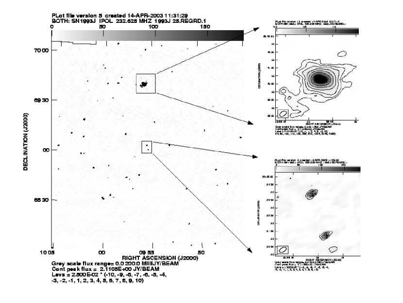
Figure 1: GMRT contour map of the field of view of SN 1993J in 243 MHz band (Observed on 2002 Mar 8). The upper square panel contains M82 and lower square panel contains the parent galactic center M81 (Top) and SN 1993J (right).

Astrophysical Image Processing System (AIPS) developed by NRAO was used to analyze all datasets with the standard GMRT data reduction. Bad antennas and corrupted data was removed using standard AIPS routines. Data were then calibrated and images of the fields were formed by Fourier inversion and CLEANing using AIPS task IMAGR (see Bhatnagar (2000, 2001) for details of data analysis procedure). For 1420 MHz and 610 MHz datasets, bandwidth smearing effects were negligible and imaging was done after averaging 100 central frequency channels (out of total 128 channels). For 325 MHz analysis, the 96 central channels (12 MHz bandwidth) were divided into 4 sub-bands of 3 MHz each for imaging. For 243 MHz analysis, we usually took 60-70 good central channels and divided them in 4 sub-bands for imaging. While making images, these sub-bands were stacked together. To take care of the wide field imaging, we divided the whole field of view in 2-5 sub fields for 1420 MHz frequency datasets, and in 5-9 sub fields in the 610 MHz datasets. For 325 MHz datasets, wide field imaging was performed with 16-25 sub fields, while for 245 MHz datasets this was done with 25-36 sub fields. We performed few rounds of phase self calibrations in all the datasets to remove the phase variations due to the bad weather and related causes and improved the images considerably. After imaging, all the subfields were combined into a single field using AIPS task FLATN. All datasets were corrected for the primary beam pattern of the antennas. Fig 1 shows the SN 1993J image on 2002 Mar 08 at 243 MHz band. The figure on the left hand panel shows the full field of view (FOV) which was imaged after dividing it in to 25 subfields and subsequently recombining. Positions of the supernova, the parent galaxy M81 and the nearby starburst galaxy M82 are shown separately in the big panels. Table 4 gives the details of the observations and analysis of all the datasets at GMRT observation epochs.

2.4 Errors in the flux density determination

Apart from the noise in the map plane (${\rm rms}\propto{[n(n-1)\Delta\nu\,\tau]}^{-1/2}$ where $n$ is the number of baselines, $\Delta\nu$ the bandwidth of the observations and $\tau$ the integration time), there are other factors which contribute to the errors in the flux density determinations. These could be modulations due to interstellar scattering and scintillation (ISS), elevation dependent errors, errors due to the bandwidth smearing and errors due to the use of two-dimensional geometry in imaging. The last two errors can be corrected for by following the procedure mentioned in the last section. Here we discuss mainly the ISS effects and elevation dependent errors which contribute to the uncertainty in the source flux density determination.

2.4.1 Interstellar scattering and scintillation

We calculated the effect of the interstellar scattering and scintillation (ISS) in the SN at all observed frequencies. Figure 1 of Walker (1998) suggests that the transition frequency ${\nu}_{0}$ (the frequency corresponding to unit scattering strength ) for the position of SN 1993J ($l=142.15,\,b=40.92$) is 8 GHz. Since all the frequencies of our observations are less than the transition frequency, the target should be in strong scattering regime. Figure 3 of Kulkarni et al. (1998) suggests that strong short-time diffractive scintillation occurs in very early stages of the supernova, when its size is still very small. Their figure suggests that SN 1993J is in the refractive interstellar scintillation (RISS) regime at the present epoch. During the GMRT observations epoch, i.e. around day 3000 since SN 1993J’s explosion, we use the size of the SN to be ${\theta}_{s}\sim 5000\,\mu$as (Bartel et al., 2002). Fresnel size of the source is ${\theta}_{r}\propto{({\nu}_{0}/\nu)}^{11/5}$ (Walker, 1998). We thus find that the SN is in the point source limit only for 243 MHz since for this frequency, ${\theta}_{s}\leq{\theta}_{r}$ (${\theta}_{r}\sim 9000\,\mu$as) and is in the extended source limit (${\theta}_{s}\geq{\theta}_{r}$) for all other frequencies (${\theta}_{r}\,{\rm is}\,\sim 4500\,\mu$as at 325 MHz, $\sim 1150\,\mu$as at 610 MHz, and $\sim 200\,\mu$ at 1420 MHz). For RISS in the point source regime, the modulation index $m_{p}$ (rms fractional flux variation) and the refractive scintillation timescale $t_{r}$ are:

$$m_{p}={(\nu/{\nu}_{0})}^{17/30}\,\,{\rm and}\,\,t_{r}({\rm hours})\propto{({\nu}_{0}/\nu)}^{11/5}$$

respectively. In the extended source regime, these factors are further modified. The modulation index is reduced by ${({\theta}_{r}/{\theta}_{s})}^{7/6}$ and refractive time scale is increased by ${\theta}_{s}/{\theta}_{r}$ (Walker, 1998). We calculate that at 243 MHz, the modulation index is 13.8%, whereas time scale of modulation is $\sim 180$ days. The modulation index and the time scale of modulation at 325 MHz are 14.7% and $\sim 100$ days respectively. At 610 MHz band, the modulation index is 4.2% whereas the time scale of variation is 100 days. At 1420 MHz, the modulation index (0.8%) is negligible and time scale of variation is 100 days. We, therefore, conclude that the interstellar scintillations and scattering are not likely to significantly modulate our flux densities on short time scales (such as $\sim 2$ months).

2.4.2 Elevation dependent errors

At high frequencies, there are noticeable changes in the antenna gains with change of elevation angle with time. Atmospheric opacity also introduces an elevation dependence on the observed visibility amplitudes. By calibrating the target source with a nearby calibrator, these variations can be accounted for to a large extent. However, if the primary flux calibrator is observed at a different elevation from the secondary gain and phase calibrator, it may lead to significant errors. Proper calibration of the flux densities at high frequencies requires the knowledge of a gain curve for the antennas, as well as the atmospheric opacity. For low frequencies such as 610, 325 and 243 MHz, elevation dependent errors are quite negligible for most of the sources. At 1420 MHz waveband, elevation dependent errors may affect the observations. However, SN 1993J is at such a high declination (69$\arcdeg$) that the data is unlikely to be severely affected by such errors. We ran AIPS task ELINT to determine the elevation dependent errors for the phase calibrators. We find that the errors are $\sim 5-6\%$ in 1420 MHz band and $\sim 2-4\%$ in 610, 325 and 243 MHz bands. However the actual errors may be a little larger than this because the program source (SN 1993J) is another 15-20^o away from the phase calibrators.

2.4.3 Calibration errors

In some of the observations, we had more than one flux calibrators. In such instances we could estimate the calibration errors in GMRT bands by using the following procedure. We assumed one flux calibrator (say $A$ ) to be the absolute calibrator and calculated the flux density of the absolute calibrator using Baars formulation. We then calibrated another flux calibrator (say $B$) with respect to the absolute calibrator ($A$) and obtained flux density of the calibrator $B$ with respect to $A$ (say $B(A)$). Since we already had the flux density of the flux calibrator $B$ using Baars formulation (say $B(Baars)$), difference of $B(A)$ and $B(Baars)$ : $\mid B(A)-B(Baars)\mid$ is an indicator of the calibration errors in GMRT. We found that the calibration errors for 1420, 610, 325 and 243 MHz bands are in the range 3-4%, 4-6%, 5-7% and 5-8% respectively.

To incorporate all the errors discussed above, we have used the following formula to quote the errors in the flux density determination for our GMRT datasets

$$\sqrt{[({\rm map\,rms})^{2}+(10\%\,{\rm of\,the\,peak\,flux\,of\,SN})^{2}]}$$

The overall error of 10% of the peak flux density at all the frequencies takes into account any possible systematic error in GMRT measurements including the small errors due to antennas’ elevation dependence. This 10% is close to the actual errors in the low frequencies 240 and 325 MHz bands but is an upper limit for the higher frequencies 1420 MHz and 610 MHz, where the overall errors are more likely to be 7-8%.

3 Results and Interpretation

3.1 Light curves of SN 1993J

In Fig. 2 we show the light curves of SN 1993J in all the frequency bands reported in Table 4. We interpret here the gross features of these light curves. The light curves in the 1420 and 610 MHz bands show a decline with time. This is the expected behavior of a supernova in the optically thin part of the light curve, where the decline is a power law in time. There appears to be a hint of a jump in the light curve somewhere between 3123 to 3296 days in the 1420 MHz frequency band. If the variation is real, the most natural explanation of this variation could be the inhomogeneity in the circumstellar medium, or non-uniform magnetic field in the plasma. Bartel et al. (2002) also found a sudden jump in the 8.4 GHz light curve around day 2000. We consider it likely that the jump in the 1420 MHz light curve referred to here is real and since the evolution of SN light curves repeat at lower frequencies at later times, the earlier jump in the 8.4 GHz light curve is being seen later in the 1.4 GHz band. However, in view of the uncertainties in the flux determinations, this conclusion is not robust at present. Future observations at lower frequencies will be a good check of the possible jumps in the SN light curve, for if jumps are real then they will show up at lower frequencies at later epochs. The 325 MHz light curve also shows a declining trend, although in a less rapid manner compared to the light curves at higher frequencies. It is likely that the supernova has just become optically thin in the 325 MHz band and hence the decline is much slower. However, the 235 MHz light curve is more or less flat, as is expected when the light curve is going through a peak. Shape of the spectral fits in radio also suggests this (see next section) and indicates that the light curve of the SN 1993J may remain flat at 235 MHz band for the next few years.

Because of a small number of data points, we do not attempt the detailed fits of the light curves with various models. However, we attempted to compare our data points with the already existing models. We used the model of synchrotron radio emission with free-free absorption (Weiler et al., 2002). The free-free absorption model for the SN 1993J light curves (Weiler et al., 2002) gives :

$$F_{\nu}({\rm mJy})=K_{1}{\left(\frac{\nu}{5\,{\rm GHz}}\right)}^{\alpha}{\left(\frac{t-t_{0}}{1\,{\rm day}}\right)}^{\beta}\,e^{-\tau}(1-e^{-{\tau}^{\prime}}){{\tau}^{\prime}}^{-1}$$ (1)

where

$$\tau=K_{2}{\left(\frac{\nu}{5\,{\rm GHz}}\right)}^{-2.1}{\left(\frac{t-t_{0}}{1\,{\rm day}}\right)}^{\delta}$$ (2)

and

$${\tau}^{\prime}=K_{3}{\left(\frac{\nu}{5\,{\rm GHz}}\right)}^{-2.1}{\left(\frac{t-t_{0}}{1\,{\rm day}}\right)}^{{\delta}^{\prime}}$$ (3)

Here $K_{1}$, $K_{2}$, and $K_{3}$ are free parameters corresponding to the flux density, uniform and non-uniform external absorption respectively at 5 GHz, one day after the explosion date $t_{0}$. Free parameters $\alpha$ and $\beta$ are the emission index and time index respectively. The parameters $\delta$, ${\delta}^{\prime}$ describe the time dependence of the optical depths for the uniform and nonuniform circumstellar media. The best fit parameter values for SN 1993J (Weiler et al., 2002) are: $K_{1}=1.86\times 10^{4}$, $\alpha=-1.07$, $\beta=-0.93$, $K_{2}=1.45\times 10^{3}$, $\delta=-2.02$, $K_{3}=6.31\times 10^{4}$, and ${\delta}^{\prime}=-2.14$. This model was fitted for high frequency VLA observations in the range 22.5 GHz to 1.4 GHz frequency bands. We extrapolate this model to 1420, 610, 325 and 243 MHz frequencies at GMRT observation epochs with the above parameters. Fig 3 shows this extrapolated light curves for the SN at 1420, 610, 325 and 243 MHz and our corresponding GMRT data points at the respective frequencies. It is evident that the free-free model described above overpredicts the flux densities at low frequencies. In fact lower the frequencies, more significant is the departure from the standard free-free model. This indicates that the optical depths fitted using high frequency datasets, simply extrapolated to low frequencies with the dependence $\tau\propto{\nu}^{-2.1}$ are not sufficient to account for the required absorption. One needs to incorporate some additional frequency dependent opacity at low frequencies, which can compensate for the difference between the model light curves and the actual data.

Since the extrapolated free-free model of Weiler et al. (2002) with the above parameters to low frequencies, say 1420, 610, 325 and 243 MHz tends to overpredict the flux density of the supernova, we incorporated an extra opacity due to synchrotron self absorption to check whether this brings the observed flux points into consistency. The SSA absorption coefficient is given as (Pacholczyk, 1970)

$${\kappa}_{SSA}=\frac{\sqrt{3}e^{3}}{8\pi m}{\left(\frac{3e}{2\pi m^{3}c^{5}}\right)}^{\gamma/2}cB^{(\gamma+2)/2}\Gamma\left(\frac{3\gamma+2}{12}\right)\Gamma\left(\frac{3\gamma+22}{12}\right){\nu}^{-(\gamma+4)/2}$$ (4)

We assumed shell size (from where radio emission is coming) to be 20% (Bartel et al., 2002) of the supernova size and used SSA optical depth as ${\tau}_{SSA}={\kappa}_{SSA}R/5$ with $R\propto t^{0.781}$ (Bartel et al., 2002). Eq. 3 is the internal absorption term, to which we add the SSA optical depth ${\tau}_{SSA}$ i.e.

$$\tau_{int}={\tau}^{\prime}+{\tau}_{SSA}$$ (5)

And the flux density of the SN including the SSA absorption is

$${F_{\nu}}^{SSA}({\rm mJy})=K_{1}{\left(\frac{\nu}{5\,{\rm GHz}}\right)}^{\alpha}{\left(\frac{t-t_{0}}{1\,{\rm day}}\right)}^{\beta}\,\left(\frac{1-e^{-{\tau}_{int}}}{{\tau}_{int}}\right)$$ (6)

where the bracketed term is the attenuation due to the total internal absorption including SSA absorption. Fig. 3 shows the light curves at 1420, 610, 325 and 243 MHz after incorporating the extra SSA opacity. We note that even after adding this extra opacity in the existing free-free model, the total optical depth is not sufficient to reproduce the observed flux density. The medium is more opaque to the radio emission at the lower frequencies.

3.2 Spectra of SN 1993J

On five different occasions we collected simultaneous or near simultaneous spectra of SN1993J by making flux density measurements at multiple frequencies separated by about a month or so. Since the supernova is $\sim$ 10 years old, we do not expect its flux density to change by significant amount in a month’s gap between the two flux density measurements. For example, using the flux density dependence on time $t$ as $F\propto t^{-0.93}$ (Weiler et al., 2002), we find that the flux density of the supernova will change only by 2% in 75 days at such late epochs. This is well within the uncertainties of the flux measurements. We also saw in the last section that the time scale of the flux density variation due to RISS is 6 months (3 months) at lower (higher) frequencies and hence RISS will not contribute significantly to the flux density variations within a month’s time gap. Therefore, we can use the observations separated by roughly a month to obtain a near-simultaneous spectrum of the SN. Table 5 gives the details of the observations used to obtain the spectra with GMRT at five different epochs.

With so few data points in the spectra it is difficult to pinpoint the synchrotron self absorption model from the free-free absorption mechanism as the dominant underlying cause of absorption. We use synchrotron self absorbed radio emission model to fit our datasets (See Chevalier (1998); Pacholczyk (1970)), which we justify in the next section.

$${f_{\nu}}^{SSA}=\frac{\pi R^{2}}{D^{2}}\frac{c_{5}}{c_{6}}B^{-1/2}{\left(\frac{\nu}{2c_{1}}\right)}^{5/2}[1-g(\nu,\gamma)]$$ (7)

where

$$g(\nu,\gamma)={\rm exp}\left[-{\left(\frac{\nu}{2c_{1}}\right)}^{-\frac{\gamma+4}{2}}\left(\frac{4fRc_{6}N_{0}B^{\frac{\gamma+2}{2}}}{3}\right)\right]$$ (8)

and

$$N_{0}=\frac{aB^{2}(\gamma-2){E_{l}}^{\gamma-2}}{8\pi}$$ (9)

The above flux density expression can be reduced to the following in the optically thin limit.

$${{f_{\nu}}^{SSA}|}_{\tau\leq 1}=\frac{4\pi fR^{3}}{3D^{2}}c_{5}N_{0}B^{(\gamma+1)/2}{\left(\frac{\nu}{2c_{1}}\right)}^{-(\gamma-1)/2}$$ (10)

And in the optically thick limit

$${{f_{\nu}}^{SSA}|}_{\tau\geq 1}=\frac{\pi R^{2}}{D^{2}}\frac{c_{5}}{c_{6}}B^{-1/2}{\left(\frac{\nu}{2c_{1}}\right)}^{5/2}$$ (11)

Here $R$ is the radius of the supernova, $D$ is the distance to the supernova, $f$ is the filling factor (which we took to be 0.5 for our purpose (Chevalier, 1998)); $\gamma$ is the electron spectral index which depends on the emission spectral index $\alpha$ as $\gamma=2\alpha+1$. $N_{0}$ is the normalization constant in the power-law distribution of electrons in $N(E)=N_{0}E^{-\gamma}$ (Chevalier, 1998), and $a$ is the equipartition factor ($a=U_{rel}/U_{B}$; $U_{rel}$ is the relativistic electron energy density, and $U_{B}$ is the magnetic energy density), and $E_{l}$ is the electron rest mass energy ($E_{l}=0.51$ MeV). The (constant) parameters $c_{1},c_{5},c_{6}$ are defined in Pacholczyk (1970); $c_{5}$, $c_{6}$ are functions of electron spectral index $\gamma$ and are tabulated in Table 7 of Appendix 2 in Pacholczyk (1970). They are:

$$c_{1}={3e\over 4\pi m^{3}c^{5}}=6.27\times 10^{18}\;\rm c.g.s.\;\rm units$$

$$c_{5}={\sqrt{3}e^{3}\over 16\pi}{e^{3}\over mc^{2}}\left({\gamma+7/3\over\gamma+1}\right)\Gamma\left({3\gamma-1\over 12}\right)\Gamma\left({3\gamma+7\over 12}\right)$$

$$c_{6}={\sqrt{3}\pi\over 72}em^{5}c^{10}\left(\gamma+{10\over 3}\right)\Gamma\left({3\gamma+2\over 12}\right)\Gamma\left({3\gamma+10\over 12}\right)$$

The parameters $R$, $B$ and $\alpha$ or $\gamma$ are the three free parameters for the fitting a model to the observed spectrum.

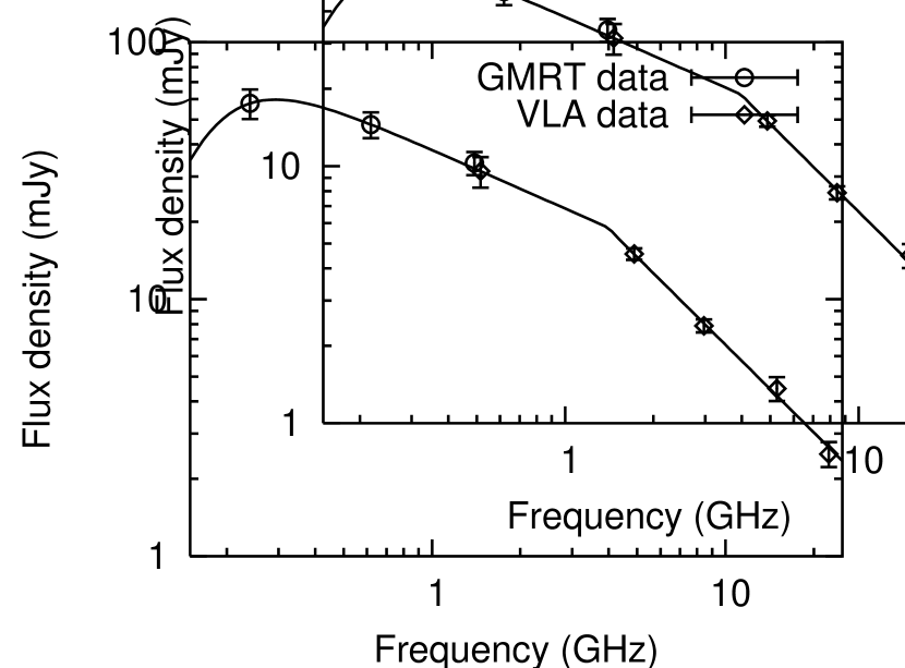
Figure 5: GMRT plus VLA combined spectrum on day 3200. Solid line is the best fit SSA model. The spectrum shows a break at 4 GHz with steepening in the spectral index by 0.62 (Chandra et al., 2004).

On day 3200, we combined the GMRT low frequency spectrum with that of high frequency VLA data (kindly provided by Kurt Weiler, C. Stockdale and their collaboration), and fit the synchrotron self absorption (SSA) model (solid line in Fig 5). We found that the spectrum at high frequency is best fit by a broken power law with a break around 4 GHz which we interpret as due to synchrotron cooling. SN 1993J is the first such young supernova where the synchrotron cooling break in the radio frequency region is seen. Observational signature of the synchrotron cooling break directly leads to the determination of the magnetic field in the plasma. This is the most direct determination of magnetic field in the shocked plasma (Chandra et al., 2004), since the age of the source is known. The lifetime of the relativistic electrons undergoing synchrotron loss is given as

$$t=\tau=E/[-{(dE/dt)}_{Sync}]=1.43\times 10^{12}B^{-3/2}{\nu}^{-1/2}_{break}\;{\rm sec}$$ (12)

Here we use ${B_{\perp}}^{2}={(B\,{\rm Sin\theta})}^{2}=(2/3)B^{2}$. However, we also include energy loss/gain due to the adiabatic expansion and the diffusive shock acceleration (Fermi acceleration) along with the synchrotron energy loss term, for the SN is young and these process are likely to be important (see Chandra et al. (2004)). Hence, the lifetime of electrons for the cumulative energy loss rate is

$$\tau=\frac{E}{{(dE/dt)}_{Total}}=\frac{E}{(R^{2}t^{-2}/20{\kappa}_{\perp})E-bB^{2}E^{2}-t^{-1}E}$$ (13)

where the second term in the denominator is synchrotron loss term with $b=1.58\times 10^{-3}$; the first term is the energy gain due to diffusive shock acceleration and the third term is the adiabatic expansion loss term. Using ${\nu}_{break}=5.12\times 10^{18}BE_{break}^{2}\;{\rm Hz}$ (Pacholczyk, 1970) in the above equation, we found the magnetic field implied by the life time argument to be $B=330$ mG. On the other hand, from the best fit with SSA, the magnetic field under equipartition assumption is $B_{eq}=38\pm 17$ mG. Comparison of the magnetic field obtained from the lifetime argument with that obtained from SSA model best fit (assuming equipartition) determines the value of the equipartition fraction between relativistic energy of particles and magnetic field energy. Equipartition fraction $a=U_{rel}/U_{mag}$ varies with magnetic field $B$ as $a=(B/B_{eq})^{-(2\gamma+13)/4}$ (Chevalier, 1998). Therefore, the fraction $a$ ranges between $8.5\times 10^{-6}\,-\,4.0\times 10^{-4}$ with a central value of $a=1.0\times 10^{-4}$ (corresponding to $B_{eq}=38$ mG) on day 3200. As Chevalier (1998) has argued, it is likely that this high magnetic field is the result of an amplification process in the interaction region and is not merely the effect of shock compression of the magnetic field in the wind by the relevant compression ratio. See Chandra et al. (2004) for a detailed study of the combined spectrum (GMRT and VLA) with the break.

The above analysis shows that if we were to fit the SSA model under the assumption of equipartition, we would end up seriously underpredicting the magnetic field, roughly an order of magnitude lower than the actual field. The relativistic plasma is far from equipartition and is strongly dominated by the magnetic energy density. We assume that the equipartition fraction, as determined above on day 3200 does not change with time. Using this fraction, we can fit the synchrotron self absorption model to our subsequent GMRT spectra and determine the most probable values of the free parameters, e.g. $R$, $B$, and $\alpha$ in the SSA model. Since we have very few data points for the spectra, we cannot determine all three parameters. Therefore we separately calculated the value of spectral index $\alpha$ using the optically thin part of the spectrum ($F_{\nu}\propto{\nu}^{-\alpha}$) between frequencies 610 MHz to 1420 MHz. The errors in the values of the spectral indices reflect the errors in the flux densities at a given frequency. The size of the supernova and the magnetic field were used thereafter as free parameters in the SSA fits to the spectra. The best fit magnetic field and the size of the supernova thus obtained and reported in Table 6 are not under the assumption of equipartition of relativistic particles and fields. Errors in $B$ and $R$ are large due to a large range in the equipartition fraction $a$ ($B\propto a^{-4/(2\gamma+13)}\,;R\propto a^{-1/(2\gamma+13)}$). Fig. 4 shows the GMRT spectra at days 3000, 3200, 3266, 3460 and 3730 since explosion. The spectrum currently appears to peak around 235 MHz due to the flattening of the light curves at these frequencies and is gradually shifting to lower frequencies. Data in the still lower frequency bands ($<235$ MHz) may constrain the peak more tightly. We estimate below some of the physical parameters of the supernova based on the spectral fits, and compare them with those determined by independent methods.

3.3 Role of synchrotron self absorption at spectral turn-over

We fit only the synchrotron self absorption model to the obtained spectra. However, we have also tried to fit the free-free absorption model to the spectra. Since there are few data points in each spectrum, these models are not easily distinguished against each other by the data. However the SSA model can be indirectly tested by comparing its predicted parameters against similar quantities measured entirely independently. For example, SN 1993J has been extensively studied using VLBI and therefore the size of the SN is known from these measurements. We also obtain the size of the SN from the SSA model using the turn-over in the spectra. Comparing the sizes obtained from these two independent methods therefore tests the SSA model. GMRT observations are only around day 3000 and later. To evaluate the SSA model at earlier epochs, we used VLA data available on Internet starting from day 65 to day 250. We digitized the VLA data for day $400-800$ from the available light curves (van Dyk et al., 1994; Fransson & Bjornsson, 1998). We also used the published data of Bartel et al. (2002) and Perez-Torres et al. (2002). We fit the SSA model to the spectra at all these epochs using the equipartition fraction derived in Chandra et al. (2004) and obtained the best fit magnetic field and size of the supernova. We compared the best fit size so obtained with that of VLBI size of SN at various epochs obtained from Fig 6 of Bartel et al. (2002). Fig 6 shows the SSA size of the supernova plotted against the VLBI size of the supernova. At late epochs beyond day 3000, no VLBI observations were available, so we have extrapolated the earlier VLBI observations to obtain the sizes of the SN at the relevant epochs, assuming the latest value of $m=0.781$ in $R\propto t^{m}$ (Bartel et al., 2002). We note that the VLBI size of the supernova and the SSA model fit size from the peak of the spectrum are largely consistent at all epochs. If SSA was not the most important absorption mechanism, the SN size determinations from the SSA model would have been smaller than the sizes obtained from VLBI (see Slysh (1990)). Since the two are roughly consistent at all epochs, the conclusion that synchrotron self absorption is the dominant absorption mechanism to determine the spectral turn-over appears natural.

We notice that at late epochs beyond day 3400, the SSA radius is more than the extrapolated VLBI size. This could be due to the incorrect estimation of the extrapolated VLBI radius with the assumed $m$, at late epochs for which VLBI observations do not exist. Additionally, uncertainties in the determination of the peak of the spectra due to the lack of very low frequency measurements may affect the accuracy of the SSA radius and associated parameters.

3.4 Evolution of spectral index, size and magnetic field

Fig 7 shows the evolution of the best fit radio spectral index $\alpha$. The spectral index evolves with time and its value changes from $\alpha\sim 0.8-1.0$ (in the first few tens of days) to $\sim 0.6$ (10 years after explosion). GMRT measurements of the spectral index have significant errors. This is because we have not fit the spectral index with SSA or FFA model since we had very few frequency data points in the spectra. Instead we calculated spectral index from the optically thin part of the GMRT spectra between frequencies 610 and 1420 MHz frequency bands, using the relation $F_{\nu}\propto{\nu}^{-\alpha}$. Errors in the determination of $\alpha$ are partly due to the errors in the flux density measurements.

Fig 8 (upper panel) shows the supernova size evolution with time. We also plot the indicative $R\propto t$ line in the Figure. It is noted that at early epochs, the size evolution is consistent with $R\propto t$, i.e. supernova ejecta expansion is free expansion while at late enough epochs, the expansion undergoes deceleration. These results are roughly consistent with those of Bartel et al. (2002) and Marcaide et al. (1997). We show the time variation of the radii determined from our SSA fits to GMRT spectra as an inset in Fig 8. The lower panel of Fig 8 shows that the magnetic field decreases as supernova ages. We also plot the indicative $B\propto t^{-1}$ line, and it suggests that within error bars, the magnetic field decreases according to $B\propto t^{-1}$ on the full time range. However there seems to be a hint of flattening in the time development between $\sim 400-1300$ days.

When synchrotron self absorption is the dominant absorption mechanism, it is not possible to estimate directly the circumstellar density, as is possible in the case of dominant external free-free absorption; but in contrast it is possible to estimate the radio supernova size, if the radio peak flux is observed. This leads to the determination of the velocities of the outer parts of the supernova, which we find from the radii reported in Table 6 to be: $v\approx 11000\,{\rm km\,s^{-1}}$ for $t\geq 3000\;\rm day$. As a comparison, note that the optical photosphere velocity decreased to $7000-10,000\;\rm\;km\;s^{-1}$ range even $10-30\;\rm day$ after explosion (Ray et al. (1993)).

3.5 Mass loss rate of the progenitor star

Estimates of the mass loss rate give crucial information about the progenitor star. Since typical ejecta velocities are $\sim 1000$ times that of wind velocities, information about mass loss rate derived a few years after the explosion can trace the history of the progenitor star a few thousands of years before the explosion. This requires an assumption about the wind velocity for the mass losing progenitor star when it exploded as a supernova. The wind velocities around red supergiant stars are $\sim 10$ km s^-1 while that of blue supergiant stars are $\sim 1000$ km s^-1. For SN 1993J, we assume in consonance with data and models (see e.g. Ray et al. (1993)) that the progenitor star had an extended red supergiant like envelope in its last stage of evolution; thus we adopt the circumstellar wind velocity to be $10$ km s^-1. We then determine the mass loss rate using the best fit parameters of SSA to the GMRT data (Table 6).

It is clear from section 3.2 that the magnetic energy density in SN 1993J considerably exceeds the relativistic particle energy density. However, these ratios are close to unity in some other supernovae, e.g. SN 2002ap (Bjornsson & Fransson, 2004), SN 1998bw (Kulkarni et al., 1998) etc. Fransson & Bjornsson (1998) have also shown that there is a rough equipartition between the magnetic energy density and the thermal energy density in the post-shock gas in SN 1993J. In turn these are related to the ram pressure of the shock front. This leads to an estimate of the mass-loss rate from the SN progenitor (Chevalier, 1998) by relating the post-shock magnetic energy density to the shock ram pressure: $B^{2}/8\pi=\zeta\rho_{0}v_{sh}^{2}$, where $\zeta$ is a numerical constant, $\rho_{0}$ is the post-shock density and $v_{sh}$ is the shock velocity. For $\zeta\leq 1$, this gives a lower limit of the estimate of the mass loss rate as

$$\dot{M}=\frac{6.6\times 10^{-5}}{m^{2}\,\zeta}\,{\left[\frac{B}{0.33\,\rm G}\right]}^{2}{\left[\frac{t}{3200\,{\rm days}}\right]}^{2}{\left[\frac{v_{w}}{10\,{\rm km\,s^{-1}}}\right]}\,{\rm{M}_{\odot}\,{yr}^{-1}}$$ (14)

Here, $m=(n-3)/(n-2)$, $n$ being ejecta density power law, is the deceleration index. Although there are no VLBI measurements for the epoch of GMRT observations, we use the extrapolated value of the latest $m$ obtained from VLBI i.e. $m=0.781$ (Bartel et al., 2002). We use the magnetic fields in the above equation that are determined from the spectral fits as given in Table 6. For $\zeta=1$, the lower limit on the mass loss rate can be calculated from Eq. 14. The values of the mass loss rate for GMRT observations thus obtained are reported in Table 7. Fig 9 shows that the mass loss rate (obtained from GMRT observations) appears to be decreasing slowly with a small slope of $1.8\times 10^{-8}{\rm{M}_{\odot}\,{yr}^{-1}/yr}$. (We assumed a constant ratio of the ejecta velocity and the wind velocity to be $v_{ej}/v_{w}\sim 1000$ to obtain the time before explosion from the epoch after explosion). Note that the predicted mass loss rate in Chevalier (1998) is constant, since it goes as $B^{2}t^{2}$ while his assumed time dependence is: $B\propto 1/t$. However, GMRT data (from day $~{}3000$ to $3730$, – a relatively short range compared to the entire data span from the date of explosion) appears to indicate a slightly steeper dependence of B on $1/t$. Although the best fit line to the mass loss rate in Fig. 9 in the narrow range of time before explosion shows a small decrement, within the error bars of the GMRT measurements of B as seen Fig 8, and on the longer timescale since explosion our results are consistent with a constant mass loss rate.

4 Summary and Conclusions

Even though SN 1993J has been one of the most well-observed targets since its explosion some 11 years ago, it continues to illuminate the physics of supernovae. SN 1993J is a unique supernova for which magnetic field and sizes are determined from model independent measurements; the former from the synchrotron cooling break and the latter from VLBI measurements. These have been utilized here to test models and parameters that determine the radio emission from this SN.

Because the radio emission from SN 1993J now peaks at frequencies lower than 235 MHz, it is necessary to observe it at lower frequencies, where the SN is still in the optically thick regime to properly determine the turn-over in the spectrum. Multifrequency spectra of SN 1993J ranging from the very low GMRT frequencies to very high VLA frequencies will thus be important observational inputs in future. The synchrotron cooling break in the combined (VLA and GMRT) spectrum on day 3200 leads to the determination of the equipartition fraction between relativistic particle and magnetic energy densities (Chandra et al., 2004). From the self consistent analysis of early spectra of SN 1993J, Fransson & Bjornsson (1998) had interpreted the rough equipartition between the nonthermal ions, the magnetic field, and the thermal energy. We affirm that the relativistic particle energy density however, is minuscule compared to the magnetic energy density in the radiating plasma.

The outer part of the supernova from where the radio emission originates is expanding at a speed of $\sim 11000\rm\;km\;s^{-1}$ for $t\geq 3000\rm days$. This speed is small compared to those found in type Ic SNe like SN 1998bw, SN 2002ap or SN 2003dh (Ray et al. (2003)) indicating that ordinary type IIb supernovae like SN 1993J have much less extreme properties than other core collapse supernovae some of which may produce gamma-ray bursts. Estimates of the mass lost from the progenitor star of SN 1993J derived from post-shock magnetic pressure and shock ram pressure and the GMRT spectra indicate that the mass loss rate remained roughly constant during 8000-10,000 years before explosion.

In our earlier paper (Chandra et al., 2003), we had argued that the size of SN 1993J determined from the SSA fits are roughly half of that obtained from VLBI measurements. However, our earlier estimates of the sizes were based on the assumption of equipartition between magnetic and relativistic particle energy densities since we did not have a direct handle on the equipartition fraction prior to the discovery of the synchrotron cooling break. In this paper we use the equipartition fraction directly determined from the synchrotron cooling break in the GMRT plus VLA spectrum on day 3200 (Chandra et al., 2004) and thereby obtain the best fit size of the SN. We now find that our derived SSA sizes roughly match the VLBI sizes of the supernova at all epochs. We thus affirm that even if free-free absorption may have had a significant contribution to the total absorption in the radio band, the peak in the spectrum is primarily determined by synchrotron self absorption. Slysh (1990) also had plotted the SSA sizes of a few supernovae against their VLBI sizes and found them to be consistent at all epochs. He thence argued that SSA alone is responsible for the turn-over in the spectra of supernovae. However his results were based on the equipartition assumption between relativistic energy density and magnetic energy density. Our results on SN 1993J confirm the conclusion of Slysh (1990), namely SSA is the main absorptive process for the turn-over, but unlike Slysh (1990) we do not assume an equipartition.

Light curves based on high frequency FFA models extrapolated to low frequencies overpredict the flux densities at low frequencies. Some extra opacity is needed to incorporate the difference. We added an extra opacity due to synchrotron self absorption which also could not fully account for the required absorption. This suggests that the low frequency opacity in SN 1993J is not a simple extrapolation of high frequency opacity and a hitherto unaccounted for absorption may be at work at low frequencies.

Bartel et al. (2002) have argued that the deceleration factor $m$ ($R\propto t^{m}$) measured with VLBI dropped from 0.92 to 0.78 around day 400 and then around day 1500, the decline of $m$ stopped and it increased to a value of 0.86. This trend was roughly mirrored in the light curves. They argue that the upturn in $m$ could be due to the SN ejecta hitting the reverse shock and exerting pressure in the forward direction. A non-uniform radial dependence of the circumstellar medium density can simultaneously provide a reasonable explanation of a non-smooth evolution of the 1420 MHz flux between day $3150-3300$. The flux density may increase if the supernova ejecta hits a clump in the CSM and decrease if the ejecta runs into a rarefied region. The enhanced emission due to the interaction with a clump may in effect lead to a flattening of the light curve rather than an actual rise, if the filling factor of the clumps is low near the radiosphere. A non-smooth evolution of the radio luminosity can also be caused by inhomogeneities in the magnetic field in the interaction region, since synchrotron emission efficiency depends on the strength of the magnetic field. The synchrotron flux density has a dependence on magnetic field as ${{f_{\nu}}^{SSA}|}_{\tau\geq 1}\propto B^{-1/2}$ in the optically thick part of the spectrum, and ${{f_{\nu}}^{SSA}|}_{\tau\leq 1}\propto B^{(\gamma+1)/2}$ in the optically thin part. Therefore, the variation in the flux density with magnetic field is less significant in the optically thick regime than in the optically thin regime. Hence, jumps in the flux densities at high frequencies will be more evident than at the lower frequencies. Due to the large errors of the measurements, one cannot ascertain whether the sudden jump in the light curve at 1420 MHz is real (though the same had been seen in 8.4 GHz light curves at earlier epochs by Bartel et al. (2002)). But if they are real, then they should be mirrored in low frequency light curves at later epochs. Further observations at low frequencies will confirm it.

Figure 2: Light curves of SN 1993J at 1420 MHz, 325 MHz bands (upper panel) and 610 MHz and 235 MHz bands (lower panel) observed with the GMRT.

Figure 3: Comparison of low frequency data to the predictions of models obtained by fitting high frequency fluxes of SN 1993J. The solid lines in all four plots are Weiler et al’s (2002) model extrapolated to lower frequencies (see sec. 3.1). Dashed lines are the flux density plots after incorporating the SSA optical depth in the Weiler et al. free-free model.

Figure 4: Best fit GMRT spectra of SN 1993J on day $\sim 3000$, 3200, 3266, 3460 and 3730 since explosion from top left in clockwise order. Solid lines are the SSA best fit models (See Table 6 for details).

Figure 6: Plot of the size of SN 1993J from SSA fit against the VLBI size. The straight line indicates the region where the SSA size equals the VLBI size of the supernova.

Figure 7: Evolution of the best fit spectral index $\alpha$ with time. Spectral index changes from $\sim 1$ to $\sim 0.6$.

Figure 8: Evolution of the size of the supernova with time (upper panel). The straight line corresponds to $R\propto t$ i.e. free expansion. Initially the expansion is free expansion but later it shows a deceleration. The inset shows the evolution of size determined only from GMRT data (note the linear scales in time and radius here). Evolution of the magnetic field in synchrotron emitting plasma with time (lower panel). Plot also shows the line corresponding to $B\propto t^{-1}$. The magnetic field evolution is roughly consistent with $B\propto t^{-1}$ though it shows some possible flattening around day 300-900.

Figure 9: Evolution of the mass loss rate of the presumed red supergiant progenitor of SN 1993J with time before explosion of the star. The solid line represents the best fit with a slope $1.8\times 10^{-8}{\rm{M}_{\odot}\,{yr}^{-1}/yr}$. Here the ratio of the ejecta velocity and wind velocity is taken to be $\sim 1000$ to compute the corresponding time before explosion.

Table 1: Details of the flux calibrators used

		Co-ordinates(J2000)			Flux Density (Jy)
Name	Redshift	RA	DEC		1420MHz	610MHz	325MHz	235MHz
3C48	0.367	$01^{\mathrm{h}}37^{\mathrm{m}}41\fs 3$	$33\arcdeg 09\arcmin 35\arcsec$		16.2	29.4	43.4	50.8
3C147	0.545	$05^{\mathrm{h}}42^{\mathrm{m}}36\fs 1$	$49\arcdeg 51\arcmin 07\arcsec$		22.3	38.3	52.7	59.2
3C286	0.849	$13^{\mathrm{h}}31^{\mathrm{m}}08\fs 3$	$30\arcdeg 30\arcmin 33\arcsec$		$-$	21.1	25.9	28.1

Table 2: GMRT observations of the phase calibrator 1035+564 at 1390 MHz band

Date of	Flux Density	Observed position J2000		Offset
Observn.	Jy$\pm$ mJy	RA	DEC	arcsec
2001 Oct 15	$2.46\pm 3.9$	$10^{\mathrm{h}}35^{\mathrm{m}}07\fs 1$	$56\arcdeg 28\arcmin 47\arcsec$	1.5″
2002 Apr 07	$2.39\pm 5.6$	$10^{\mathrm{h}}35^{\mathrm{m}}07\fs 0$	$56\arcdeg 28\arcmin 48\arcsec$	1.0″
2002 Jun 24	$2.08\pm 2.9$	$10^{\mathrm{h}}35^{\mathrm{m}}06\fs 9$	$56\arcdeg 28\arcmin 47\arcsec$	1.5″
2002 Sep 21	$2.33\pm 3.3$	$10^{\mathrm{h}}35^{\mathrm{m}}07\fs 1$	$56\arcdeg 28\arcmin 46\arcsec$	1.8″
2003 Jun 13	$1.89\pm 1.6$	$10^{\mathrm{h}}35^{\mathrm{m}}07\fs 0$	$56\arcdeg 28\arcmin 47\arcsec$	0.0″

Table 3: Details of the GMRT observations of phase calibrator 0834+555

Date of	Frequency	Flux Density	Observed position J2000		Offset
Observn.	MHz	Jy$\pm$ mJy	RA	DEC	arcsec
2000 Nov 08	1420	$8.80\pm 8.5$	$08^{\mathrm{h}}34^{\mathrm{m}}54\fs 9$	$55\arcdeg 34\arcmin 24\arcsec$	3.0″
2000 Dec 16	1420	$8.75\pm 6.6$	$08^{\mathrm{h}}34^{\mathrm{m}}55\fs 0$	$55\arcdeg 34\arcmin 14\arcsec$	7.1″
2001 Jun 02	1390	$8.71\pm 4.2$	$08^{\mathrm{h}}34^{\mathrm{m}}52\fs 2$	$55\arcdeg 34\arcmin 38\arcsec$	43.9″
2001 Mar 24	610	$8.47\pm 17.8$	$08^{\mathrm{h}}34^{\mathrm{m}}54\fs 9$	$55\arcdeg 34\arcmin 34\arcsec$	13.0″
2001 Aug 24	610	$8.18\pm 12.6$	$08^{\mathrm{h}}34^{\mathrm{m}}55\fs 1$	$55\arcdeg 34\arcmin 20\arcsec$	1.8″
2001 Dec 30	610	$8.74\pm 13.8$	$08^{\mathrm{h}}34^{\mathrm{m}}54\fs 9$	$55\arcdeg 34\arcmin 22\arcsec$	1.0″
2002 Mar 08	610	$8.23\pm 12.5$	$08^{\mathrm{h}}34^{\mathrm{m}}54\fs 9$	$55\arcdeg 34\arcmin 21\arcsec$	0.0″
2002 May 19	610	$8.44\pm 20.0$	$08^{\mathrm{h}}34^{\mathrm{m}}54\fs 9$	$55\arcdeg 34\arcmin 21\arcsec$	0.0″
2002 Sep 16	610	$8.50\pm 11.3$	$08^{\mathrm{h}}34^{\mathrm{m}}54\fs 9$	$55\arcdeg 34\arcmin 21\arcsec$	0.0″
2003 Jun 17	610	$8.14\pm 15.7$	$08^{\mathrm{h}}34^{\mathrm{m}}54\fs 9$	$55\arcdeg 34\arcmin 21\arcsec$	0.0″
2001 Jul 05	325	$8.96\pm 26.6$	$08^{\mathrm{h}}34^{\mathrm{m}}55\fs 0$	$55\arcdeg 34\arcmin 24\arcsec$	3.4″
2002 Mar 07	325	$8.76\pm 6.8$	$08^{\mathrm{h}}34^{\mathrm{m}}55\fs 0$	$55\arcdeg 34\arcmin 22\arcsec$	1.8″
2002 Aug 16	325	$9.06\pm 31.9$	$08^{\mathrm{h}}34^{\mathrm{m}}54\fs 9$	$55\arcdeg 34\arcmin 21\arcsec$	0.0″
2001 Dec 31	243	$8.77\pm 46.8$	$08^{\mathrm{h}}34^{\mathrm{m}}54\fs 9$	$55\arcdeg 34\arcmin 21\arcsec$	0.0″
2002 Mar 08	243	$8.20\pm 36.6$	$08^{\mathrm{h}}34^{\mathrm{m}}55\fs 0$	$55\arcdeg 34\arcmin 24\arcsec$	3.4″
2002 Sep 16	243	$9.02\pm 43.8$	$08^{\mathrm{h}}34^{\mathrm{m}}55\fs 0$	$55\arcdeg 34\arcmin 20\arcsec$	1.8″
2003 Jun 17	243	$8.25\pm 44.7$	$08^{\mathrm{h}}34^{\mathrm{m}}54\fs 9$	$55\arcdeg 34\arcmin 21\arcsec$	0.0″

Table 4: Details of the GMRT observations of SN 1993J

Date of	Days since	Freq. Band	No. of good	Resolution	Flux density	rms
Observn	explosion	MHz	Antennas	arcsec	mJy	mJy
2000 Nov 08	2779	1420	19	25x18	$35.1\pm 3.5$	0.5
2000 Dec 16	2818	1420	23	8x5	$36.1\pm 3.6$	0.3
2001 Jun 02	2988	1390	28	4x3	$32.7\pm 3.3$	0.2
2001 Oct 15	3123	1390	24	10x6	$33.9\pm 3.3$	0.3
2002 Apr 07	3296	1390	25	11x7	$24.6\pm 3.7$	1.0
2002 Jun 24	3374	1390	19	6x3	$23.4\pm 2.5$	0.4
2002 Sep 21	3463	1390	25	5x3	$24.2\pm 2.4$	0.2
2003 Jun 13	3728	1280	24	5x2	$20.2\pm 2.1$	0.2
2001 Mar 24	2917	610	20	11x7	$56.1\pm 5.5$	0.5
2001 Aug 24	3072	610	24	13x7	$55.8\pm 5.7$	0.4
2001 Dec 30	3198	610	20	11x8	$47.8\pm 5.5$	1.9
2002 Mar 08	3266	610	25	14x6	$44.4\pm 4.5$	0.3
2002 May 19	3338	610	24	18x8	$44.6\pm 4.5$	0.6
2002 Sep 16	3458	610	26	10x6	$37.5\pm 3.8$	0.4
2003 Jun 17	3732	610	23	14x5	$33.4\pm 4.3$	0.8
2001 Jul 05	3022	325	18	19x10	$69.2\pm 15.8$	2.5
2002 Mar 07	3265	325	24	19x13	$55.8\pm 7.4$	1.9
2002 Aug 16	3427	325	16	18x9	$61.8\pm 8.8$	2.7
2001 Dec 31	3199	243	20	19x14	$57.8\pm 7.6$	2.5
2002 Mar 08	3266	243	17	26x16	$60.9\pm 10.8$	4.1
2002 Sep 16	3458	243	17	26x16	$56.7\pm 8.7$	4.0
2003 Jun 17	3732	243	22	23x11	$58.2\pm 11.8$	5.4

Table 5: Details of the near simultaneous spectra of SN 1993J

Date of	Days since	Freq. Band	Flux density	rms
Obs.	explosion	MHz	mJy	mJy
2001 Jul 05	3022	325	$69.2\pm 15.8$	2.5
2001 Aug 24	3072	610	$55.8\pm 5.7$	0.4
2001 Jun 02	2988	1390	$32.7\pm 3.3$	0.2
2001 Dec 31	3199	243	$57.8\pm 7.6$	2.5
2001 Dec 30	3198	610	$47.8\pm 5.5$	1.9
2001 Oct 15	3123	1390	$33.9\pm 3.5$	0.3
2002 Jan 13	3212	1460	$31.44\pm 4.28$	2.9
2002 Jan 13	3212	4885	$15\pm 0.77$	0.19
2002 Jan 13	3212	8440	$7.88\pm 0.46$	0.24
2002 Jan 13	3212	14965	$4.49\pm 0.48$	0.34
2002 Jan 13	3212	22485	$2.50\pm 0.28$	0.13
2002 Mar 08	3266	243	$60.9\pm 10.8$	4.1
2002 Mar 07	3265	325	$56.2\pm 7.4$	1.9
2002 Mar 08	3266	610	$44.4\pm 4.5$	0.3
2002 Apr 07	3296	1390	$24.6\pm 3.7$	1.0
2002 Sep 16	3458	243	$56.7\pm 8.7$	4.0
2002 Sep 16	3458	610	$37.5\pm 3.8$	0.4
2002 Sep 21	3463	1390	$24.2\pm 2.4$	0.2
2003 Jun 17	3732	243	$58.2\pm 11.8$	5.4
2003 Jun 17	3732	610	$33.4\pm 4.3$	0.8
2003 Jun 13	3728	1280	$20.2\pm 2.1$	0.2

Table 6: Best fit parameters of SSA fits to the GMRT spectra

Days since	Spectral index	SSA best fit
explosion	$\alpha$	$B$ Gauss	$R\times 10^{17}$ cm
3000	$0.65\pm 0.17$	$0.28\pm 0.12$	$2.71\pm 0.43$
3200	$0.51\pm 0.21$	$0.43\pm 0.19$	$3.26\pm 0.41$
3266	$0.71\pm 0.22$	$0.24\pm 0.11$	$3.11\pm 0.58$
3460	$0.53\pm 0.17$	$0.19\pm 0.09$	$4.10\pm 0.50$
3730	$0.68\pm 0.21$	$0.15\pm 0.07$	$4.83\pm 0.69$

Table 7: Lower limits to the mass loss rates of the progenitor of SN 1993J from Eq. 14 with m=0.781

Days since	Years before	Mass Loss Rate
explosion	explosion	$10^{-5}\,{\rm M_{\odot}Yr^{-1}}$
3000	8219	$6.8\pm 1.3$
3200	8767	$10.2\pm 3.6$
3266	8948	$5.9\pm 1.2$
3460	9480	$4.2\pm 0.9$
3730	10219	$3.01\pm 0.7$

References

- Baars et al. (1977) Baars, J.W.M., Genzel, R., Pauliny-Toth & I.I.K., Witzel,A. 1977 A&A, 61, 99
- Bartel et al. (2002) Bartel, N., Bietenholz,M.F., Rupen, M.P., et al 2002 ApJ, 581, 404
- Bhatnagar (2000) Bhatnagar, S. 2000, MNRAS, 317, 453
- Bhatnagar (2001) Bhatnagar, S. 2001, Ph.D. thesis, Univ. of Pune & Tata Inst. of Fundamental Research
- Bjornsson & Fransson (2004) Bjornsson, C., Fransson, C. 2004, ApJ, 605, 823
- Chandra et al. (2004) Chandra, P., Ray, A., & Bhatnagar, S. 2004, ApJ, 604, L97
- Chandra et al. (2003) Chandra, P., Ray. A, & Bhatnagar, S., 2003b, astro-ph/0311418, To appear in proceedings of IAU Colloquium 192 ”Supernovae (10 years of SN 1993J)”,April 2003, Valencia, Spain, eds. J. M. Marcaide and K. W. Weiler
- Chevalier & Fransson (2003) Chevalier, R., Fransson, C. 2003, Supernovae and Gamma-Ray Bursters, ed. K. Weiler. Lecture Notes in Physics, Vol. 598. Berlin, New York: Springer, 2003, p.171
- Chevalier (1998) Chevalier, R. 1998 ApJ, 499, 810
- Freedman et al. (1994) Freedman, W.L., Hughes, S.M., Madore, B.F., et al. 1994, ApJ, 427, 628
- Fillipenko et al. (1993) Filippenko, A.V., Matheson, T., & Woosley, S. E. 1993 IAU circ. no. 5787
- Höflich et al. (1993) Höflich, P., Langer, N., & Duschinger, M. 1993, A& A, 275, L29
- Fransson & Bjornsson (1998) Fransson, C., Bjornsson, C. 1998 ApJ, 509, 861
- Kulkarni et al. (1998) Kulkarni, S.R., Frail, D.A., Wieringa, M.H., & Ekers, R.D. et al. 1998, Nature, 395, 663
- Marcaide et al. (1997) Marcaide, J. M., Alberdi, A., Ros, E. et al 1997, ApJ, 486, L31
- Maund et al. (2004) Maund, J. R., Smartt, S.J., Kudritzki, R. P. et al. 2004, Nature, 427, 129
- Nomoto et al. (1993) Nomoto, K., Suzuki, T., Shigeyama, et al. 1993, Nature, 364, 507
- Pacholczyk (1970) Pacholczyk, A.G., 1970 Radio Astrophysics: Nonthermal Processes in Galactic and Extragalactic Sources (San Francisco: Freeman)
- Perez-Torres et al. (2002) Perez-Torres, M.A., Alberdi, A., & Marcaide, J.M. 2002 A&A, 394, 71
- Podsiadlowsky et al. (1993) Podsiadlowsky, P.H., Hsu, J.J.L., Joss, P.C., & Ross, R.R. 1993, Nature, 364, 509
- Ray et al. (2003) Ray, A., Chandra, P., Sutaria, F.K., & Bhatnagar, S. 2003, astro-ph/0311419 to appear in proceedings of IAU Colloquium 192 ”Supernovae (10 years of SN 1993J)”, April 2003, Valencia, Spain, eds. J. M. Marcaide and K. W. Weiler
- Ray et al. (1993) Ray, A., Singh, K.P., & Sutaria, F.K. 1993, J. Astroph. Astron., 14, 53
- Ripero et al. (1993) Ripero, J., Garcia, F., & Rodriguez, D. 1993, IAU Circ. No. 5731
- Swartz et al. (1993) Swartz, D.A., Clocchiatti, A., Benjamin, R., et al. 1993, Nature, 365, 232
- Slysh (1990) Slysh, V.I. 1990, Sov. Astron. Lett., 16, 339
- Utrobin (1994) Utrobin, V. 1994 A & A, 281, L89
- van Dyk et al. (2002) Van Dyk, S.D., Garnavich, P.M., Filippenko, A.V., & Hoeflich, P. 2002, PASP, 114, 1322
- van Dyk et al. (1994) van Dyk, S. D., Weiler, K., Sramek, R., et al. 1994 ApJL, 432, 115
- Walker (1998) Walker, M.A. 1998, MNRAS, 294, 307
- Weiler et al. (1993) Weiler, K.W., Sramek, R.A., Rupen, M.P. & Panagia, N. 1993, IAU Circ. No. 5752
- Weiler et al. (2002) Weiler, K.W., Panagia, N., Montes, J.M., & Sramek, R.A. 2002, ARA&A, 40, 387
- Weiler et al. (1991) Weiler, K.W., van Dyk, S.D., Discenna, J.L., Panagia, N., et al. 1991, ApJ, 380, 161
- Woosley et al. (1994) Woosley, S.E., Eastman, R.G., Weaver, T.A., Pinto, P.A., 1994, ApJ, 429, 300
- Zimmermann et al. (1993) Zimmermann, H.-U., Lewin, W., Magnier, E., et al. 1993, IAU Circ. No. 5748 & 5750