Figure Rotation of Cosmological Dark Matter Halos

Abstract

We have analyzed galaxy and group-sized dark matter halos formed in a high resolution $\mathrm{\Lambda}$CDM numerical N-body simulation in order to study the rotation of the triaxial figure, a property in principle independent of the angular momentum of the particles themselves. Such figure rotation may have observational consequences, such as triggering spiral structure in extended gas disks. The orientation of the major axis is compared at 5 late snapshots of the simulation. Halos with significant substructure or that appear otherwise disturbed are excluded from the sample. We detect smooth figure rotation in 278 of the 317 halos in the sample. The pattern speeds follow a log normal distribution centred at $\Omega_{p}=0.148~{}h~{}\mathrm{km~{}s^{-1}~{}kpc^{-1}}$ with a width of 0.83. These speeds are an order of magnitude smaller than required to explain the spiral structure of galaxies such as NGC 2915 (catalog ). The axis about which the figure rotates aligns very well with the halo minor axis, and also reasonably well with its angular momentum vector. The pattern speed is correlated with the halo spin parameter $\lambda$, but shows no correlation with the halo mass. The halos with the highest pattern speeds show particularly strong alignment between their angular momentum vectors and their figure rotation axes. The figure rotation is coherent outside 0.12 $r_{\mathrm{vir}}$. The measured pattern speed and degree of internal alignment of the figure rotation axis drops in the innermost region of the halo, which may be an artifact of the numerical force softening. The axis ratios show a weak tendency to become more spherical with time.

1 Introduction

Although there have been many theoretical studies of the shapes of cosmological dark matter halos (e.g. Dubinski & Carlberg, 1991; Warren et al., 1992; Cole & Lacey, 1996; Jing & Suto, 2002), there has been relatively little work done on how those figure shapes evolve with time, in particular, whether the orientation of a triaxial halo stays fixed, or whether the figure rotates. While the orientation of the halo can clearly change during a major merger, it is not known whether the orientation changes in between cataclysmic events. Absent any theoretical prediction one way or the other, it is usually assumed that the figure orientation of triaxial halos remain fixed when in isolation (e.g. Subramanian, 1988; Johnston et al., 1999; Lee & Suto, 2003)

Early work at detecting figure rotation in simulated halos was done by Dubinski (1992) (hereafter D92). While examining the effect of tidal shear on halo shapes, he found that in all 14 of his 1–$2\times 10^{12}~{}\mathrm{M_{\sun}}$ halos, the direction of the major axis rotated uniformly around the minor axis. The period of rotation varied from halo to halo, and ranged from 4 Gyr at the fast end to 50 Gyr at the slow end, or equivalently the angular velocities ranged between 0.1 and 1.6 $\mathrm{km~{}s^{-1}~{}kpc^{-1}}$. It is difficult to draw statistics from this small sample size, especially since the initial conditions of this simulation were not drawn from cosmological models, but were performed in a small isolated box with the linear tidal field of the external matter prescriptively superimposed (Dubinski & Carlberg, 1991). Given that the main result of D92 is that the tidal shear may have a significant impact on the shapes of halos, it is clearly important to do such studies using self-consistent cosmological initial conditions.

Recent studies of figure rotation come from Bureau et al. (1999) (BFPM99) and Pfitzner (1999) (P99). P99 compared the orientation of cluster mass halos in two snapshots spaced 500 Myr apart in an SCDM simulation ($\Omega=1$, $\Lambda=0$, $h=0.5$). He detected rotation of the major axis in $\sim 5\%$ of them, and argued that the true fraction with figure rotation is probably higher. BFPM99 presented one of these halos which was extracted from its cosmological surroundings and left to evolve in isolation for 5 Gyr. During that time, the major axis rotated around the minor axis uniformly at all radii at a rate of 60° $\mathrm{Gyr^{-1}}$, or about 1 $\mathrm{km~{}s^{-1}~{}kpc^{-1}}$.

There may be observational consequences to a dark matter halo whose figure rotates. BFPM99 suggested that triaxial figure rotation is responsible for the spiral structure of the blue compact dwarf galaxy NGC 2915 (catalog ). Outside of the optical radius, NGC 2915 (catalog ) has a large H I disk extending to over 22 optical disk scale lengths (Meurer et al., 1996). The gas disk shows clear evidence of a bar, and a spiral pattern extending over the entire radial extent of the disk. BFPM99 argue that the observed gas surface density is too low for a bar or spiral structure to form by gravitational instability, and that there is no evidence of an interacting companion to trigger the pattern. They propose that the pattern may instead be triggered by a rotating triaxial halo.

Bekki & Freeman (2002) followed this up with Smoothed Particle Hydrodynamics (SPH) simulations of a disk inside a halo whose figure rotates, and showed that a triaxial halo with a flattening of $b/a=0.8$ and a pattern speed of $3.84~{}\mathrm{km~{}s^{-1}~{}kpc^{-1}}$ could trigger spiral patterns in the disk. Masset & Bureau (2003) (hereafter MB03) found that in detail, the observations of NGC 2915 (catalog ) are better fit by increasing the disk mass by an order of magnitude (for example, if most of the hydrogen is molecular, e.g. Pfenniger, Combes, & Martinet, 1994), but that a triaxial halo with $b/a\approx 0.85$ and a pattern speed of between 6.5 and $8.0~{}\mathrm{km~{}s^{-1}~{}kpc^{-1}}$ also provides an acceptable fit.

MB03 concluded that if the halo were undergoing solid body rotation at this rate, its spin parameter would be $\lambda\approx 0.157$, which is extremely large (only $5\times 10^{-3}$ of all halos have spin parameters at least that large). However, this argument may be flawed because the figure rotation is a pattern speed, not the speed of the individual particles which constitute the halo, and so it is in principle independent of the angular momentum; in some cases the figure may even rotate retrograde to the particle orbits (Freeman, 1966). Schwarzschild (1982) discusses in detail the orbits inside elliptical galaxies with figure rotation. He finds that models can be constructed from box and $X$-tube orbits, which have no net streaming of particles with respect to the figure (though they have prograde streaming at small radius and retrograde streaming at large radius), and so result in figures and particles with the same net rotation. He also constructs models that include prograde-streaming $Z$-tube orbits, which result in a figure that rotates slower than the particles. Stable retrograde $Z$-tube orbits also exist, but Schwarzschild (1982) did not attempt to include them in his models, so it may also be possible for the figure to rotate faster than the particles. While these results demonstrate the independence of the figure and particle rotation, it is not clear if they can be translated directly to dark matter halos. Dark matter halos may have different formation mechanisms and may be subject to different tidal forces than elliptical galaxies, and the different density profile may also have a large effect on the viable orbital families (Gerhard & Binney, 1985).

If there are observational consequences to dark halo figure rotation, such as those found by Bekki & Freeman (2002), they can be used as a direct method to distinguish between dark matter and models such as MOdified Newtonian Dynamics (MOND) that propose to change the strength of the force of gravity (Milgrom, 1983; Sanders & McGaugh, 2002). Many of the traditional methods of deducing dark matter cannot easily distinguish between the presence of a roughly spherical dark matter halo and a modified force or inertia law. However, a major difference between dark matter and MOND is that dark matter is dynamical, and so tests that detect the presence of dark matter in motion are an effective tool to discriminate between these possibilities. Among the tests that can make this distinction are the ellipticities of dark matter halos as measured using X-ray isophotes, the Sunyaev-Zeldovich effect, and weak lensing (Buote et al., 2002; Lee & Suto, 2003, 2004; Hoekstra et al., 2004); the presence of bars with parameters consistent with being stimulated by their angular momentum exchange with the halo (Athanassoula, 2002; Valenzuela & Klypin, 2003); and spatial offset between the baryons and the mass in infalling substructure measured using weak lensing (Clowe, Gonzalez, & Markevitch, 2004). Rotation of the halo figure requires that dark matter is dynamic, and therefore observable structure triggered by figure rotation potentially provides another test of the dark matter paradigm.

In this paper, we use cosmological simulations to determine how the figures of $\mathrm{\Lambda}$CDM halos rotate. The organization of the paper is as follows. Section 2 presents the cosmological simulations. Section 3 describes the method used to calculate the figure rotations, which are presented in Section 4. Finally we discuss our conclusions in Section 5.

2 The Simulations

The halos are drawn from a large high resolution cosmological N-body simulation performed using the GADGET2 code (Springel et al., 2001). We adopt a “concordance” cosmology (e.g. Spergel et al., 2003) with $\Omega_{0}=0.3$, $\Omega_{\Lambda}=0.7$, $\Omega_{\mathrm{bar}}=0.045$, $h=0.7$, and $\sigma_{8}=0.9$. The only effect of $\Omega_{\mathrm{bar}}$ is on the initial power spectrum, since no baryonic physics is included in the simulation. The simulation contains $512^{3}=134,217,728$ particles in a periodic volume $50~{}h^{-1}$ Mpc comoving on a side. All results are scaled into $h$-independent units when possible. The full list of parameters is given in Table 1.

Table 1: Parameters of the cosmological simulation.

Parameter	Value
$N$	$512^{3}$
Box size ($h^{-1}~{}\mathrm{Mpc}$ comoving)	$50$
Particle mass ($10^{7}~{}h^{-1}~{}\mathrm{M_{\sun}}$)	7.757
Force softening length ($h^{-1}~{}\mathrm{kpc}$)	5
Hubble parameter $h$ ($H_{0}=100~{}h~{}\mathrm{km~{}s^{-1}~{}Mpc^{-1}}$)	0.7
$\Omega_{0}$	0.3
$\Omega_{\Lambda}$	0.7
$\sigma_{8}$	0.9
$\Omega_{\mathrm{bar}}$	0.045

A friends-of-friends algorithm is used to identify halos (Davis et al., 1985). We use the standard linking length of

$$b=0.2\bar{n}^{-1/3},$$ (1)

where $\bar{n}=N/V$ is the global number density.

Measuring the figure rotation requires comparing the same halo at different times during the simulation. We analyze snapshots of the simulation at lookback times of approximately 1000, 500, 300, and 100 $h^{-1}~{}\mathrm{Myr}$ with respect to the $z=0$ snapshot. The scale factor $a$ of each snapshot, along with its corresponding redshift and lookback time, is listed in Table 2.

Table 2: Snapshots used to calculate figure rotations.

Snapshot Name	Scale Factor	Redshift	Lookback Time
	($a$)	($z$)	($h^{-1}~{}\mathrm{Myr}$)
b090	0.89	0.1236	1108
b096	0.95	0.0526	496
b098	0.97	0.0309	296
b100	0.99	0.0101	98
b102	1.0	0.0	0

3 Methodology

3.1 Introduction

The basic method is to identify individual halos in the final $z=0$ snapshot of the simulation, to find their respective progenitors in slightly earlier snapshots, and to measure the rotation of the major axes through their common plane as a function of time.

Precisely determining the direction of the axes is crucial and difficult. When merely calculating axial ratios or internal alignment, errors on the order of a few degrees are tolerable. However, if a pattern speed of 1 $\mathrm{km~{}s^{-1}~{}kpc^{-1}}$, as observed in the halo of BFPM99, is typical, then a typical halo will only rotate by 4° in between the penultimate and final snapshots of the simulation. Therefore, the axes of a halo must be determined more precisely than this in order for the figure rotation to be detectable. In fact, we should strive for even smaller errors to see if slower-rotating halos exist. It would have been difficult for P99 to detect halos rotating much slower than the halo presented in BFPM99; although the error varies from halo to halo (for reasons discussed in section 3.3), Figure 5.23 of P99 shows that most of his halos had orientation errors of between 8° and 15°, corresponding to a minimum resolvable figure rotation of $\sim 0.6~{}\mathrm{km~{}s^{-1}~{}kpc^{-1}}$ for a $2\sigma$ detection in snapshots spaced 500 Myr apart.

A major difficulty in determining the principal axes so precisely is substructure. The orientation of a mass distribution is usually found by calculating the moment of inertia tensor $I_{ij}=\sum_{k}m_{k}r_{k,i}r_{k,j}$, and then diagonalizing $I_{ij}$ to find the principal axes. However, this procedure weights particles by $r^{2}$. Therefore, substructure near the edge of the halo (or of the subregion of the halo used to calculate the shape) can exert a large influence on the shape of nearly spherical halos, especially if a particular subhalo is part of the calculation in one snapshot but not in another, such as when it has just fallen in. This is particularly problematic because subhalos are preferentially found at large radii (Ghigna et al., 2000; De Lucia et al., 2004; Gill et al., 2004; Gao et al., 2004). Moving substructures can also induce a false measurement of figure rotation due to their motion within the main halo at approximately the circular velocity.

To mitigate this, we firstly use particles in a spherical region of radius 0.6 $r_{\mathrm{vir}}$ surrounding the center of the halo, rather than picking the particles from a density dependent ellipsoid as in Warren et al. (1992) or Jing & Suto (2002). We find that those methods allow substructure at one particular radius to influence the overall shape of the ellipsoid from which particles are chosen for the remainder of the calculation, and therefore bias the results even when other measures are adopted to minimize their effect. The choice of a spherical region biases the derived axis ratios toward spherical values, but does not affect the orientation. Secondly, the particles are weighted by $1/r^{2}$ so that each mass unit contributes equally regardless of radius (Gerhard, 1983). Both D92 and P99 take similar approaches, but using radii based on ellipsoidal shells. Therefore, we base our analysis on the principal axes of the reduced inertia tensor

$$\tilde{I}_{ij}=\sum_{k}\frac{r_{k,i}r_{k,j}}{r_{k}^{2}}.$$ (2)

In the majority of halos, the substructure is a small fraction of the total mass, usually less than 5% of the total mass within 60% of the virial radius (De Lucia et al., 2004, Figure 8), so its effect is much reduced. There are still some halos which have not yet relaxed from a recent major merger, in which case the “substructure” constitutes a significant fraction of the halo. To find these cases, the reduced inertia tensor is separately calculated enclosing spheres of radius 0.6, 0.4, 0.25, 0.12, and 0.06 times the virial radius to look for deviations as a function of radius (see section 5 for details). These radii are always with respect to the $z=0$ value of $r_{\mathrm{vir}}$.

We find that only halos with at least $4\times 10^{3}$ particles, or masses of at least $\sim 3\times 10^{11}~{}h^{-1}~{}\mathrm{M_{\sun}}$ have sufficient resolution for the orientation of the principal axis to be determined at sufficient precision (see Section 3.3). There are 1432 halos in the $z=0$ snapshot satisfying this criterion, with masses extending up to $2.8\times 10^{14}~{}h^{-1}~{}\mathrm{M_{\sun}}$.

3.2 Halo matching

Figure 1: Histogram of the fraction of the final mass that comes from the b096 ($z\approx 0.05$, solid line) and b090 ($z\approx 0.12$, dashed line) halo which contributes the most mass.

To match up the halos at $z=0$ with their earlier counterparts, we use the individual particle numbers provided by GADGET which are invariant from snapshot to snapshot, and find which halo each particle belongs to in each snapshot. The progenitor of each $z=0$ halo in a given $z>0$ snapshot is the halo that contributes $\geq 90\%$ of the final halo mass. Sometimes no such halo exists; in these cases, the halo has only just formed or underwent a major merger and so is not useful for our purposes. Figure 1 shows a histogram of the fraction of the final halo mass that comes from the b096 ($z\approx 0.05$) halo which contributes the most mass. There are also some cases where two nearby objects are identified as a single halo in an earlier snapshot but as distinct objects in the final snapshot. We therefore impose the additional constraint that the mass contributed to the final halo must also be $\geq 90\%$ of the progenitor’s mass. In the longer time between the earliest snapshot b090 and the final snapshot b102, a halo typically accretes a greater fraction of its mass, and so a more liberal cut of 85% is used for this snapshot (see the dashed histogram in Figure 1). 492 of the halos that satisfied the mass cut did not have a progenitor which satisfied these criteria in at least one of the $z>0$ snapshots and so were eliminated from the analysis, leaving a sample of 940 matched halos.

3.3 Error in axis orientation

There are two sources of errors that enter into the determination of the axes: how well the principal axes of the particle distribution can be determined, and whether that particle distribution has a smooth triaxial figure. Here we estimate the error assuming that it is not biased by substructure. The halos for which this assumption does not hold will become apparent later in the calculation.

For a smooth triaxial ellipsoid represented by $N$ particles, the error is a function of $N$ and of the intrinsic shape: as the axis ratio $b/a$ or $c/b$ approaches unity, the axes become degenerate. To quantify this, we have performed a bootstrap analysis of the particles in a sphere of radius 0.6 $r_{\mathrm{vir}}$ of each $z=0$ halo (Heyl et al., 1994). If the sphere contains $N$ particles then we resample the structure by randomly selecting $N$ particles from that set allowing for duplication and determine the axes from this bootstrap set. We do this 100 times for each halo. The dispersion of these estimates around the calculated axis is taken formally as the “$1\sigma$” angular error, and is labelled $\theta_{\mathrm{boot}}$.

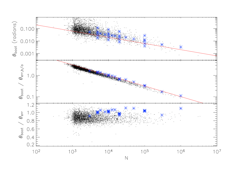
Figure 2: Angular bootstrap error $\theta_{\mathrm{boot}}$ as a function of the number of particles $N$ within the central 0.6 $r_{\mathrm{vir}}$ of each halo. Points are the cosmological halos, and asterisks are randomly sampled smooth NFW halos. (Top): Angular error $\theta_{\mathrm{boot}}$. The solid line is the fit $\theta_{\mathrm{err},N}$ from equation (3). (Middle): Ratio between the angular error and the error expected for the halo given its axis ratio $b/a$, i.e. $\theta_{\mathrm{boot}}/\theta_{\mathrm{err},b/a}$. The solid line is $\theta_{\mathrm{err},N}$ from equation (3) renormalized to the typical error of 0.02 radians. (Bottom): Ratio between the angular error and the analytic estimate $\theta_{\mathrm{err}}$ from equation (5).

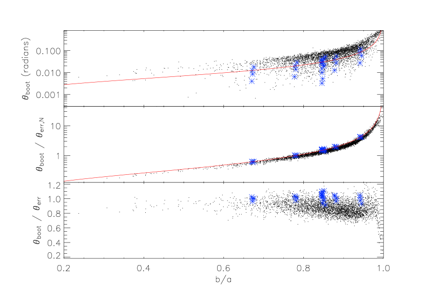
Figure 3: Angular bootstrap error $\theta_{\mathrm{boot}}$ as a function of the axis ratio $b/a$ of each halo. Points are the cosmological halos, and asterisks are randomly sampled smooth NFW halos. (Top): Angular error $\theta_{\mathrm{boot}}$. The solid line is the fit $\theta_{\mathrm{err},b/a}$ from equation (4). (Middle): Ratio between the angular error and the error expected for the halo given the number of particles $N$, i.e. $\theta_{\mathrm{boot}}/\theta_{\mathrm{err},N}$. The solid line is $\theta_{\mathrm{err},b/a}$ from equation (4) renormalized to the typical error of 0.02 radians. (Bottom): Ratio between the angular error and the analytic estimate $\theta_{\mathrm{err}}$ from equation (5).

As expected, the two important parameters are $N$ and the axis ratio. We focus here on the major axis, for which the important axis ratio is $b/a$. The top panels of Figures 2 and 3 show the dependence of the bootstrap error on $N$ and $b/a$ respectively for all halos with $M>10^{11}~{}h^{-1}~{}\mathrm{M_{\sun}}$. The solid lines are empirical fits:

$$\theta_{\mathrm{err},N}=\frac{2}{\sqrt{N}},$$ (3)

and

$$\theta_{\mathrm{err},b/a}=0.005\frac{\sqrt{b/a}}{1-b/a}.$$ (4)

The form of equation (3) is not surprising; if a smooth halo was randomly sampled, we would expect the errors to be Poissonian with an $N^{-1/2}$ dependence. However, the cosmological halos are not randomly sampled. Individual particles “know” where the other particles are, because they have acquired their positions by reacting in the potential defined by those other particles. Therefore, the errors may be less than expected from a randomly sampled halo. To test this, we construct a series of smooth prolate NFW halos (Navarro, Frenk, & White, 1996) with $b/a$ axis ratios ranging from 0.5 to 0.9, randomly sampled with between $3\times 10^{3}$ and $3\times 10^{5}$ particles, and perform the bootstrap analysis identically for each of these halos as for the cosmological halos. Because the method for calculating axis ratios outlined in Section 3.1 biases axis ratios toward spherical, the recovered $b/a$ of these randomly sampled halos is larger than the input value, and ranges from 0.65 to 0.95. The errors for these randomly sampled smooth halos are shown as asterisks in Figures 2 and 3.

The top panel of Figure 2 shows a rise in the dispersion of the error for $N\lesssim 4000$, with many halos having errors greater than the 0.1 radians necessary to detect the figure rotation of the halo presented in BFPM99. Therefore, we only use halos with $N>4000$.

The bootstrap error appears to be completely determined by $N$ and $b/a$. The residuals of $\theta_{\mathrm{boot}}$ with respect to $\theta_{\mathrm{err},N}$ are due to $\theta_{\mathrm{err},b/a}$ and vice versa. This is shown in the middle panels of Figures 2 and 3. In the middle panel of Figure 2 we have divided out the dependence of $\theta_{\mathrm{boot}}$ on the axis ratio, making apparent an extremely tight relation between the residual and $N$, while in the middle panel of Figure 3 we have divided out the dependence of $\theta_{\mathrm{boot}}$ on $N$, showing the equally tight relation between the residual and $b/a$. It is apparent from comparing the points and asterisks that the errors in the cosmological halos are slightly smaller than for randomly sampled smooth halos.

Combining equations (3) and (4), and noting that the typical error is $\theta_{\mathrm{boot}}\approx 0.02$ radians, we find the bootstrap error is well fit by

$$\theta_{\mathrm{err}}=\frac{1}{2\sqrt{N}}\frac{\sqrt{b/a}}{1-b/a}.$$ (5)

The bottom panels of Figures 2 and 3 show the residual ratio between the bootstrap error $\theta_{\mathrm{boot}}$ and the analytic estimate $\theta_{\mathrm{err}}$. The vast majority of points lie between 0.8 and 1.0, indicating that $\theta_{\mathrm{err}}$ overestimates the error by $\sim 10\%$. Equation (5) breaks down as $b/a$ approaches unity; these halos are nearly oblate and so do not have well-defined major axes. It also becomes inaccurate at very low $b/a$ due to low-mass poorly-resolved halos. Even in these cases, the error estimate is conservative, but to be safe we have eliminated axes with $b/a<0.35$ or $b/a>0.95$ from the subsequent analysis, regardless of the nominal error. The randomly-sampled smooth halos follow equation (5) extremely well, so the non-Poissonianity of the sampling in simulated halos reduces the errors by 10%.

Calculating the bootstraps is computationally expensive, so equation (5) is used for the error in all further computation. Because this estimate is expected to be correct for smooth ellipsoids, cases where the error is anomalous are indications of residual substructure.

3.4 Figure rotation

Figure 4: Diagram that demonstrates how we fit a plane to the major axis measurements at all snapshots (thick lines) and then find the increase of phase $\phi$ as a function of time. The figure rotation axis is perpendicular to the best fit plane, and defined such that $\phi$ increases around it counter-clockwise with time.

Ideally one would fit the figure rotation by comparing the orientation of the axis at each snapshot to that of a unit vector rotating uniformly along a great circle, and minimize the $\chi^{2}$ to find the best fit uniform great circle trajectory. However, this requires minimizing a non-linear function in a four-dimensional parameter space, a non-trivial task. We adopt the simpler and numerically more robust method of solving for the plane $z=ax+by$ that fits the major axis measurements of the halo best at all timesteps, assuming the error is negligible. The change of the phase of the axes in this plane as a function of time are then fit by linear regression. A schematic diagram of this process is shown in Figure 4.

The degree to which the axes are consistent with lying in a plane is checked by calculating the out-of-plane $\chi^{2}$:

$$\chi^{2}_{\mathrm{oop}}\equiv\frac{1}{\nu}\sum_{i}\frac{\Delta\theta_{i}^{2}}{{\theta_{\mathrm{err}}}_{i}^{2}},$$ (6)

where $\nu$ is the number of degrees of freedom and $\Delta\theta_{i}$ is the minimum angular distance between the major axis at timestep $i$ and the great circle defined by the best fit plane.

Because the axes have reflection symmetry, it is impossible to measure a change in phase of more than $\pi/2$. The phases are adjusted by units of $\pi$ such that the difference in phase between adjacent snapshots is always less than $\pi/2$. If the figure were truly rotating by 90° or more in between the snapshots, it would be impossible to accurately measure this rotation since the angular frequency would be larger than the Nyquist frequency of our sampling rate. Any faster pattern speeds would be aliased to lower angular velocities, with an aliased angular velocity of $\Omega_{\mathrm{Nyq}}-(\Omega_{p}-\Omega_{\mathrm{Nyq}})$, where $\Omega_{p}$ is the intrinsic angular velocity of the pattern and $\Omega_{\mathrm{Nyq}}$ is the Nyquist frequency. For snapshots spaced $500~{}h^{-1}~{}\mathrm{Myr}$ apart, the maximum time between the snapshots we analyze, the maximum detectable angular velocity is 3.8 $h~{}\mathrm{km~{}s^{-1}~{}kpc^{-1}}$. We do not expect the figure to change so dramatically as we have excluded major mergers. However, this can be checked post facto by checking whether the distribution of measured angular velocities extends up to the Nyquist frequency; if so, then there are likely even more rapidly rotating figures whose angular frequency is aliased into the detectable range, fooling us into thinking they are rotating slower. If the measured distribution does not extend to the Nyquist frequency, then it is unlikely that there are any figures rotating too rapidly to be detected (see Section 4).

The best fit linear relation for the phase as a function of time is found by linear regression. Because the component of an isotropic angular error projected onto a plane is half of the isotropic error, we divide the error of equation (5) by two before we perform the regression. The slope of the linear fit gives the pattern speed $\Omega_{p}$ of the figure rotation. The error is the $1\sigma$ limit on the slope.

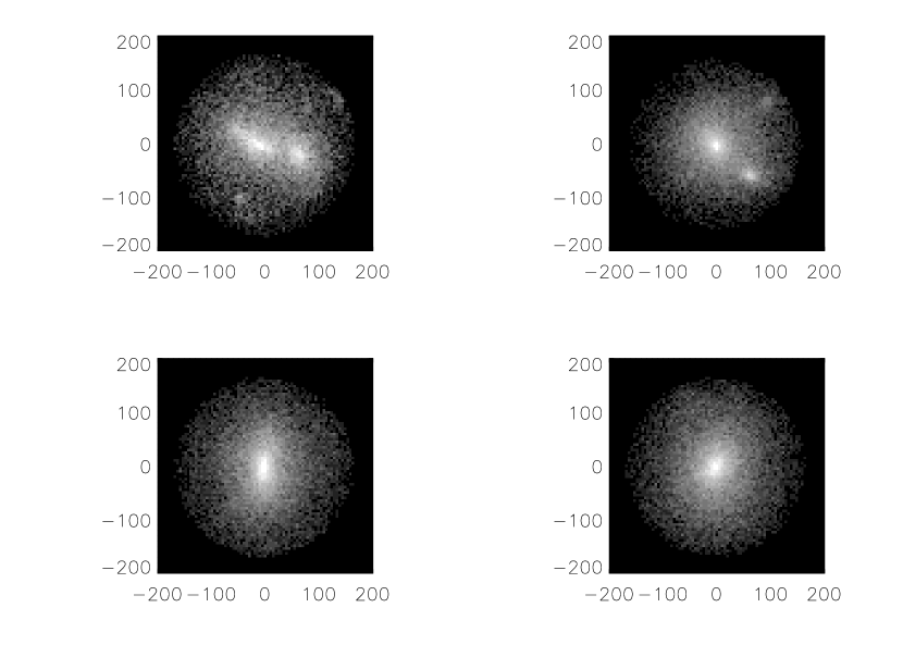
Figure 5: Log-weighted projected density of 4 halos with a range of subhalo fractions $f_{s}$. The subhalo fractions are 0.166 (top-left), 0.065 (top-right), 0.045 (bottom-left), and 0.016 (bottom-right). Axes are in units of $h^{-1}~{}\mathrm{kpc}$ from the halo center. All halos have masses in the range $2$ – $3\times 10^{12}~{}h^{-1}~{}\mathrm{M_{\sun}}$.

Once we have calculated the pattern speed for each halo, we can eliminate the cases where substructure has severely impacted the results. In these cases, the signal is dominated by a large subhalo at a particular radius, so the derived pattern speed will be significantly different when the sphere is large enough to include the subhalo from when the subhalo is outside the sphere. We have calculated the pattern speed using enclosing spheres of radius 0.6, 0.4, 0.25, 0.12, and 0.06 of the virial radius. The fraction of mass in subhalos can be estimated via the change in the pattern speed $\Omega_{p}$ at adjacent radii. Because the reduced inertia tensor is mass-weighted, the figure rotation of a sphere with a smooth component rotating at $\Omega_{p,\mathrm{smooth}}$ plus a subhalo containing a fraction $f_{s}$ of the total mass moving at the circular velocity $v_{c}$ at radius $R~{}r_{\mathrm{vir}}$ is approximately

$$\Omega_{p}\approx(1-f_{s})\Omega_{p,\mathrm{smooth}}+f_{s}\frac{v_{c}}{R~{}r_{\mathrm{vir}}},$$ (7)

where the difference due to the presence of the subhalo is

$$\Delta\Omega_{p}=f_{s}\frac{v_{c}}{R~{}r_{\mathrm{vir}}}=f_{s}\sqrt{\frac{GM(<R~{}r_{\mathrm{vir}})}{R^{3}~{}r_{\mathrm{vir}}^{3}}}.$$ (8)

If the density profile is roughly isothermal, the enclosed mass is

$$M(<R~{}r_{\mathrm{vir}})=\frac{4}{3}\pi\Delta_{c}\rho_{\mathrm{crit}}R~{}r_{\mathrm{vir}}^{3}.$$ (9)

Solving equations (8) and (9) gives an expression for the fraction of the mass in substructure given a jump of $\Delta\Omega_{p}$ in the measured pattern speed when crossing radius $R~{}r_{\mathrm{vir}}$:

$$f_{s}=\frac{\Delta\Omega_{p}R}{\sqrt{\frac{4}{3}\pi G\Delta_{c}\rho_{\mathrm{crit}}}}.$$ (10)

The term in the square root is equal to $0.72~{}h~{}\mathrm{km~{}s^{-1}~{}kpc^{-1}}$. For each halo, we compute the value of $f_{s}$ due to the jump $\Delta\Omega_{p}$ between each set of adjacent radii, i.e. for $R=0.4,0.25,0.12,$ and 0.06, and adopt the largest value of $f_{s}$ as the substructure fraction of the halo. Figure 5 shows log-weighted projected densities of 4 halos in the mass range $2$ – $3\times 10^{12}~{}h^{-1}~{}\mathrm{M_{\sun}}$ with a variety of values of $f_{s}$, ranging from 0.166 at the top-left to 0.016 at the bottom right. After examining a number of halos spanning a range of $f_{s}$, we adopt a cutoff of $f_{s}<0.05$ for undisturbed halos. This eliminates 289 of the 940 halos, leaving 651 undisturbed halos.

A further 158 halos were eliminated because the angular error approached $\pi/2$ in at least one of the snapshots. This includes the halos with $b/a<0.35$ or $b/a>0.95$ discussed in Section 3.3. We also eliminate cases where the reduced $\chi^{2}$ from the linear fit of phase versus time indicates that the intrinsic error of the direction determination is much lower than suggested by equation (5), indicating that the model of the halo as a smooth ellipsoid is violated (10 halos with $\chi^{2}_{\nu}<0.1$), and those cases where the phase does not evolve linearly with time (134 halos with $\chi^{2}_{\nu}>10$). Finally, we eliminate halos where the axes do not lie on a common plane, i.e. the 32 halos where $\chi^{2}_{\mathrm{oop}}>10$. Therefore, the final sample consists of 317 halos.

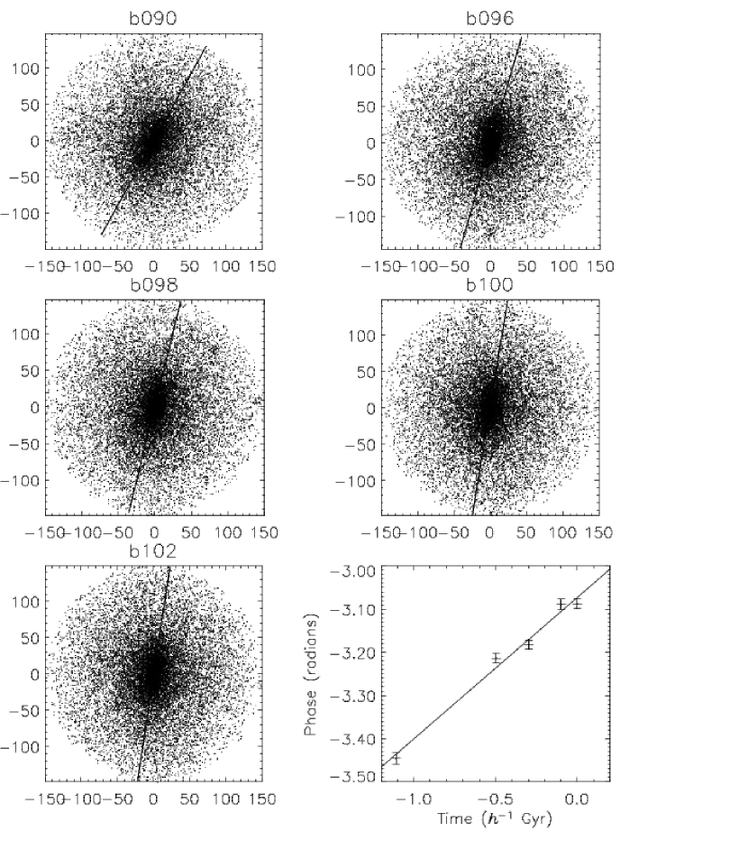
Figure 6: (Upper-left five panels): Projection onto the best fit plane of the inner 0.6 $r_{\mathrm{vir}}$ of a sample halo at the five snapshots we analyze. Axes are in units of $h^{-1}~{}\mathrm{kpc}$ from the halo center. From left to right, top to bottom, the snapshots are at 1108, 496, 296, 98, and 0 $h^{-1}~{}\mathrm{Myr}$ before $z=0$. The solid line is the major axis, which rotates counterclockwise by 20° from beginning to end. (Bottom-right): Phase of the major axis in the rotational plane of the sample halo. The zero point is arbitrary, but identical in all snapshots. The solid line is the linear fit, with a slope of $0.33~{}h~{}\mathrm{radians~{}Gyr^{-1}}$.

A sample halo is shown in the first five panels of Figure 6. It was chosen randomly from the halos with relatively low errors and typical pattern speeds. It has a mass of $1.9\times 10^{12}~{}h^{-1}~{}\mathrm{M_{\sun}}$, and a pattern that rotates at $0.32\pm 0.01~{}h~{}\mathrm{km~{}s^{-1}~{}kpc^{-1}}$. It has a spin parameter $\lambda=0.047$, and axis ratios of $b/a=0.86$ and $c/a=0.77$ at $z=0$. The derived substructure fraction is $f_{s}=0.045$, and the out-of-plane $\chi^{2}_{\mathrm{oop}}=8.5$. The solid line shows the measured major axis in each snapshot, which rotates counterclockwise in this projection. The phase of its figure rotation as a function of time is shown in the bottom-right panel of Figure 6. The zero point is arbitrary, but is consistent from snapshot to snapshot. The linear fit is also shown, which has a reduced $\chi^{2}$ of 2.9.

4 Results

Figure 7: Measured pattern speed of the rotation of the major axis. The $x$-axis is the error in the pattern speed. The solid line shows where the measure pattern speed is equal to the estimated error, while the dashed line is the $2\sigma$ limit. The horizontal dotted line shows the Nyquist limit.

Figure 8: Histogram of the pattern speeds of the figure rotation, expressed in $\log\Omega_{p}$. The thin histogram contains all halos that have $2\sigma$ detections of figure rotation, i.e. those above the dashed line of Figure 7, and is incomplete at $\Omega_{p}<0.126~{}h~{}\mathrm{km~{}s^{-1}~{}kpc^{-1}}$ or equivalently $\log\Omega_{p}<-0.9$. The thick histogram contains only those halos with errors less than 0.01 $h~{}\mathrm{km~{}s^{-1}~{}kpc^{-1}}$, and is incomplete at $\Omega_{p}<0.015~{}h~{}\mathrm{km~{}s^{-1}~{}kpc^{-1}}$ or $\log\Omega_{p}<-1.8$. The dashed curves are Gaussian fits to the histograms. The vertical dotted line shows the Nyquist limit.

Figure 9: Fractional histogram of pattern speeds of the figure rotation, expressed linearly in $\Omega_{p}$. The thin histogram contains all halos that have $2\sigma$ detections of figure rotation (incomplete at $\Omega_{p}<0.126~{}h~{}\mathrm{km~{}s^{-1}~{}kpc^{-1}}$), while the thick histogram contains halos with errors less than 0.01 $h~{}\mathrm{km~{}s^{-1}~{}kpc^{-1}}$and is complete down to $\Omega_{p}=0.015~{}h~{}\mathrm{km~{}s^{-1}~{}kpc^{-1}}$. The dashed curve is the log normal fit given by equation (11).

Figure 7 shows the measured figure rotation speeds for all of the halos in the sample, as a function of their error. Halos with measured pattern speeds less than twice as large as the estimated error (the dashed line) are taken as non-detections. 278 of the 317 halos have detected figure rotation. A histogram of the pattern speeds is presented in Figure 8, expressed in $\log\Omega_{p}$. The thin histogram contains all halos with $2\sigma$ detections, while the thick histogram contains those with the smallest errors, less than 0.01 $h~{}\mathrm{km~{}s^{-1}~{}kpc^{-1}}$. The largest upper limit due to a non-detection in the main sample is $\Omega_{p}<0.126$ ($\log\Omega_{p}<-0.9$), so the thin histogram is incomplete below this level, while the low error sample contains only one upper limit, $\Omega_{p}<0.015$ ($\log\Omega_{p}<-1.8$), so the thick histogram is complete down to this level. The dashed curves are Gaussian fits to the histograms. The fit to the thin histogram, which has the largest sample size but is incomplete at low $\Omega_{p}$, peaks at $\log\Omega_{p}=-0.80$ and has a standard deviation of 0.29, while the thick curve, which contains fewer halos but is less biased toward large values of $\Omega_{p}$, peaks at $\log\Omega_{p}=-0.84$ and has a standard deviation of 0.34. We give more weight to the thick histogram, whose points all have very small errors, and propose that the true distribution peaks at $\log\Omega_{p}=-0.83$ with a standard deviation of 0.36. Expressed as a log normal distribution, the probability is

$$P(\Omega_{p})=\frac{1}{\Omega_{p}\sigma\sqrt{2\pi}}\exp\left(-\frac{\ln^{2}(\Omega_{p}/\Omega_{p_{0}})}{2\sigma^{2}}\right),$$ (11)

where $\Omega_{p_{0}}=10^{-0.83}=0.148~{}h~{}\mathrm{km~{}s^{-1}~{}kpc^{-1}}$ and the natural width $\sigma=0.36\ln 10=0.83$. This fit is shown in Figure 9, compared to the fractional distribution of halos in the full (thin) and low error (thick) samples, and encompasses both the large number of halos with low $\Omega_{p}$ seen when the errors are sufficiently small, and the tail at high $\Omega_{p}$ seen when the sample size is sufficiently large.

For comparison, the halo in BFPM99 has a pattern speed of 2 $h~{}\mathrm{km~{}s^{-1}~{}kpc^{-1}}$. This lies slightly above the top end of our distribution; the maximum pattern speed in our sample is 1.01 $h~{}\mathrm{km~{}s^{-1}~{}kpc^{-1}}$. Based on the log normal fit of equation (11), we estimate the fraction of halos with $\Omega_{p}\geq 2~{}h~{}\mathrm{km~{}s^{-1}~{}kpc^{-1}}$ to be $\sim 10^{-3}$. Therefore, this halo is unusual, but it is not unreasonable to find a halo with such a pattern speed in a large simulation. Given the size of the errors in P99, and that he found very few halos with figure rotation, it should not be surprising that P99 could only detect pattern speeds at the upper end of the overall distribution. The different adopted cosmologies may also influence the results (note, however, that this comparison is performed in $h$-independent units). Our results are also mostly consistent with D92, who finds pattern speeds of between 0.1 and 1.6 $\mathrm{km~{}s^{-1}~{}kpc^{-1}}$ in a sample of 14 halos. We have trouble reproducing the most rapidly rotating halos in D92, but this may be a product of the heuristic initial conditions in D92 compared to the cosmological initial conditions we use.

In order to account for the spiral structure in NGC 2915 (catalog ), a triaxial figure would need to rotate at $7\pm 1~{}\mathrm{km~{}s^{-1}~{}kpc^{-1}}$ (MB03). This is almost an order of magnitude faster than the fastest of the halos in our sample, and the log normal fit from equation (11) suggests that the fraction of halos with $\Omega_{p}\geq 6~{}\mathrm{km~{}s^{-1}~{}kpc^{-1}}$ is $5\times 10^{-7}$. Therefore, the figure rotation of undisturbed $\mathrm{\Lambda}$CDM halos can not explain the spiral structure of NGC 2915 (catalog ). SPH simulations of gas disks inside triaxial halos with pattern speeds of 0.77 $\mathrm{km~{}s^{-1}~{}kpc^{-1}}$, comparable to the fastest pattern speeds in our sample, show very weak if any enhancement of spiral structure compared to a static halo (Bekki & Freeman, 2002, Figure 2f). Therefore, it is unlikely that triaxial figure rotation can be detected in extended gas disks.

Figure 10: As in Figure 7, but only including snapshots b096 through b102.

The dotted line in both Figures 7 and 8 shows the Nyquist frequency of 3.8 $h~{}\mathrm{km~{}s^{-1}~{}kpc^{-1}}$. If the measured distribution of pattern speeds extended up to the Nyquist frequency, the intrinsic distribution would likely extend above the Nyquist frequency, and the results would be affected by frequency aliasing. However, the measured distribution does not approach the Nyquist frequency. Therefore, any halo whose figure rotation is aliased would need to be wildly anomalous, with a pattern speed many times faster than any other halo in our sample. We consider this unlikely. Figure 10 shows the pattern speeds as a function of the error, as in Figure 7, except that it only uses snapshots b096 through b102, so the maximum time between snapshots is 200 $h^{-1}~{}\mathrm{Myr}$, and the corresponding Nyquist frequency is 7.6 $h~{}\mathrm{km~{}s^{-1}~{}kpc^{-1}}$, shown again as the dotted line. The top of the distribution does not change between Figures 7 and 10, demonstrating that the results are not affected by aliasing.

Figure 11: (Top): Histogram of the direction cosine between the minor axis of the halo and the figure rotation axis, for halos with $2\sigma$ detections of figure rotation. Because the minor axis has reflection symmetry, this is always positive. (Bottom): Direction cosine as a function of the magnitude of figure rotation.

We investigate how the figure rotation axis relates to two other important axes. Both D92 and P99 claim that the major axis rotates around the minor axis. The direction cosine between the rotation axis and the minor axis is plotted both as a function of the pattern speed and as a histogram in Figure 11. We confirm that the rotation axis coincides very strongly with the minor axis. Due to the tendency for the halos to be prolate, the minor and intermediate axes tend to degenerate, accounting for some (but not all) of the misaligned tail.

Figure 12: (Top): Histogram of the direction cosine between the angular momentum vector of the halo and the figure rotation axis, for halos with $2\sigma$ detections of figure rotation. (Bottom): Direction cosine as a function of the magnitude of figure rotation.

The rotation axis is compared to the angular momentum vector of the halo in Figure 12. Because the angular momentum is usually well aligned with the minor axis of halos (Warren et al., 1992), it is no surprise that the rotation axis is also well aligned with the angular momentum vector. Because the alignment between the minor axis and angular momentum of halos is not perfect (Warren et al. (1992), Bailin & Steinmetz, in preparation), some of the halos with perfectly aligned figure rotation and minor axes have less perfect alignment between the figure rotation axis and the angular momentum vector, seen as the bump in Figure 12 that extends down to a direction cosine of 0.6; the tail of the distribution extends all the way to anti-alignment. The alignment is also plotted as a function of the pattern speed in the lower panel of Figure 12. There is no trend for the halos with slow figure rotation, but all but two of the halos with $\Omega_{p}>0.4~{}h~{}\mathrm{km~{}s^{-1}~{}kpc^{-1}}$ have figure rotation axes and angular momentum vectors that are well aligned, with a direction cosine of 0.65 or higher.

Figure 13: Pattern speed of the figure rotation versus the mass of the halo. Error bars are $1\sigma$ errors for halos with at least $2\sigma$ detections of figure rotation. The upper limits are the halos with a measured $\Omega_{p}<2\sigma$, and are plotted at the $2\sigma$ limit.

Figure 14: Pattern speed of the figure rotation versus the spin parameter of the halo. Error bars and upper limits are as in Figure 13.

We have attempted to see if the pattern speed is correlated with other halo properties, in particular its mass and its angular momentum. Figure 13 shows the pattern speed of the figure rotation versus the halo mass. Error bars are $1\sigma$ errors, with $2\sigma$ upper limits plotted for halos which lie below the dashed line of Figure 7. There is no apparent correlation between the halo mass and its pattern speed.

Figure 14 shows the pattern speed versus the spin parameter $\lambda$, where

$$\lambda\equiv\frac{J\left|E\right|^{1/2}}{GM^{5/2}}$$ (12)

(Peebles, 1969). We use the computationally simpler $\lambda^{\prime}$ as an estimate for $\lambda$, where

$$\lambda^{\prime}\equiv\frac{J}{\sqrt{2}MVR}$$ (13)

(Bullock et al., 2001). There is a tendency for halos with fast figure rotation to have large spin parameters; in particular, all but one of the halos with $\Omega_{p}>0.4~{}h~{}\mathrm{km~{}s^{-1}~{}kpc^{-1}}$ have $\lambda>0.024$. These are the same halos which are shown to have particularly well-aligned rotation axes and angular momentum vectors in Figure 12. We have calculated the median value of $\Omega_{p}$ including the upper limits for bins of width $\Delta\lambda=0.01$. The median rises steadily from 0.12 $h~{}\mathrm{km~{}s^{-1}~{}kpc^{-1}}$ for $\lambda<0.02$ to 0.44 $h~{}\mathrm{km~{}s^{-1}~{}kpc^{-1}}$ for $\lambda>0.06$. Note that P99 only detected figure rotation in halos with $\lambda>0.05$ (see his Figure 5.24).

Figure 15: Direction cosine between the angular momentum vector of the halo and the figure rotation axis versus the spin parameter $\lambda$.

The degree of alignment between the figure rotation axis and the angular momentum vector may depend on the angular momentum content of the halo. Figure 15 shows how this alignment depends on the spin parameter $\lambda$. There is no trend for $\lambda<0.05$, but the halos with $\lambda>0.05$ show particularly good alignment. This is a natural consequence of the tendency for halos with rapid figure rotation to have well aligned figure rotation and angular momentum axes (Figure 12), and the correlation between figure pattern speed and spin parameter $\lambda$ (Figure 14).

Figure 16: Pattern speed of figure rotation $\Omega_{p}$ at 0.4, 0.25, 0.12, and 0.06 of the virial radius $r_{\mathrm{vir}}$ (top to bottom) as a function of the pattern speed at $0.6~{}r_{\mathrm{vir}}$. Only halos where both radii in the comparison contain at least 4000 particles, pass all of the tests of Section 5, and have $2\sigma$ detections of figure rotation are included. All units are $h~{}\mathrm{km~{}s^{-1}~{}kpc^{-1}}$. The solid line corresponds to equal pattern speeds.

Figure 17: Histogram of the direction cosine of the alignment between the figure rotation axis of the halo as a whole ($r<0.6~{}r_{\mathrm{vir}}$) and of just the inner 0.4, 0.25, 0.12, and 0.06 of the virial radius $r_{\mathrm{vir}}$ (top to bottom). Only halos where both radii in the comparison contain at least 4000 particles, pass all of the tests of Section 5, and have $2\sigma$ detections of figure rotation are included.

Figures 16 and 17 show how the figure rotation changes with radius. Figure 16 shows how the pattern speeds at different radii are related, while Figure 17 shows the alignment of the figure rotation axes between radii. Each panel includes only the halos that have at least 4000 particles within the inner radius, pass all of the tests of Section 5 for both radii, and have $2\sigma$ measurements of figure rotation at both radii. Due to the smaller number of particles in spheres of smaller radii, there are progressively fewer halos with good measurements at smaller radii. The top panels show that the figure rotation in the outer regions of the halo is very coherent. To some degree, this is by construction; the test for substructure is equivalent to a cut in $\Delta\Omega_{p}$ between adjacent radii. However, gradual drifts of $\Omega_{p}$ and changes in the figure rotation axis with radius are still possible. The lower panels of Figures 16 and 17 show that this indeed happens. In particular, while the figure rotation within 0.12 $r_{\mathrm{vir}}$ and 0.6 $r_{\mathrm{vir}}$ are strongly correlated, the pattern speeds within 0.12 $r_{\mathrm{vir}}$ are slightly smaller and the alignment of the rotation axes is not quite as strong. The bottom panels show that in the innermost regions, within 0.06 $r_{\mathrm{vir}}$, the pattern speeds are significantly smaller than for the halo as a whole, particularly for those halos with high pattern speeds, and more than half of the halos show no alignment between the figure rotation axes.

We examine three possible explanations for these trends with radius. First, it may be that the halos with high pattern speeds are still affected by residual substructure in the outer regions. However, the gradual decline for all halos seen as the radius shrinks suggests that the mechanism responsible for the difference affects all halos equally and gradually, rather than affecting a few halos at a specific radius. Another piece of evidence that argues against this explanation is that the halos with the highest measured pattern speeds do not have preferentially high values of $f_{s}$; they have values evenly spread between 0 and the cutoff of 0.05. A second possibility is that the figure rotation, although steady on timescales of 1 Gyr, may be fundamentally a transitory feature caused by a tidal encounter or the most recent major merger. The inner region of the halo has a shorter dynamical time, and therefore the effects of such a disturbance will be erased faster in the inner regions than the outer regions. This is consistent with the gradual decrease in pattern speed with radius and the decrease in alignment. However, the halo of BFPM99 has fast figure rotation (faster than any of our halos), and yet shows steady figure rotation at all radii for 5 Gyr. We propose instead that the effects of force softening are becoming important at the smaller radii. The radius of the innermost sphere for the halos plotted in the bottom panels of Figures 16 and 17 range from 3–5 force softening lengths, where the effects of the gravitational softening can still be important (Power et al., 2003). The weaker gravitational force results in a more spherical potential, consistent with the weaker figure rotation and lack of alignment.

Figure 18: Fractional rate of change of the $b/a$ (left) and $c/a$ (right) axis ratio of the halos in the sample, as a function of the $z=0$ axis ratio.

We have calculated the rate of change of the $b/a$ and $c/a$ axis ratios over the 5 snapshots using linear regression. The evolution of the axis ratios with time is linear for almost all halos. Figure 18 shows the fractional rate of change, $(\dot{b/a})/(b/a)$ and $(\dot{c/a})/(c/a)$, of the axis ratios as a function of the value of the axis ratio in the final snapshot. The median and standard deviation of the distribution of $(\dot{b/a})/(b/a)$ are $0.0089~{}h~{}\mathrm{Gyr^{-1}}$ and $0.0349~{}h~{}\mathrm{Gyr^{-1}}$ respectively. For $c/a$, they are $0.0093~{}h~{}\mathrm{Gyr^{-1}}$ and $0.0297~{}h~{}\mathrm{Gyr^{-1}}$ respectively. Therefore, there is a weak tendency for undisturbed halos to become more spherical with time. Most halos require several Gyr before their flattening changes significantly; there are, however, a few outliers with quite significant changes in their axis ratios. Figure 18 demonstrates that there is no trend of $(\dot{b/a})/(b/a)$ or $(\dot{c/a})/(c/a)$ with the value of the axis ratio except for the outliers with very high (low) values of $\dot{b/a}$, which could not have such high (low) rates of change if the values of $b/a$ were not very high (low) in the final snapshot. We find no trend with any other halo property such as mass, spin parameter, pattern speed, substructure fraction, or alignment of the figure rotation axis with the angular momentum vector or minor axis.

5 Conclusions

We have detected rotation of the orientation of the major axis in most undisturbed halos of a $\mathrm{\Lambda}$CDM cosmological simulation. The axis around which the figure rotates is very well aligned with the minor axis in most cases. It is also usually well aligned with the angular momentum vector. The distribution of pattern speeds is well fit by a log normal distribution,

$$P(\Omega_{p})=\frac{1}{\Omega_{p}\sigma\sqrt{2\pi}}\exp\left(-\frac{\ln^{2}(\Omega_{p}/\Omega_{p_{0}})}{2\sigma^{2}}\right),$$ (14)

with $\Omega_{p_{0}}=0.148~{}h~{}\mathrm{km~{}s^{-1}~{}kpc^{-1}}$ and $\sigma=0.83$.

The pattern speed $\Omega_{p}$ is correlated with spin parameter $\lambda$. The median pattern speed rises from 0.12 $h~{}\mathrm{km~{}s^{-1}~{}kpc^{-1}}$ for halos with $\lambda<0.02$ to 0.44 $h~{}\mathrm{km~{}s^{-1}~{}kpc^{-1}}$ for halos with $\lambda>0.06$, with a spread of almost an order of magnitude around this median at a given value of $\lambda$. The 11% of halos in the sample with the highest pattern speeds, $\Omega_{p}>0.4~{}h~{}\mathrm{km~{}s^{-1}~{}kpc^{-1}}$, not only have large spin parameters, but also show particularly strong alignment between their figure rotation axes and their angular momentum vectors. There is no obvious correlation of the figure rotation properties with mass. The pattern speed and figure rotation axis is coherent in the outer regions of the halo. Within 0.12 $r_{\mathrm{vir}}$, the pattern speed drops, particularly for those halos with fast figure rotation, and the internal alignment of the figure rotation axis deteriorates. This is probably an artifact of the numerical force softening.

BFPM99 hypothesized that the spiral structure in NGC 2915 (catalog ) is due to figure rotation of a triaxial halo. The required pattern speed of $7\pm 1~{}\mathrm{km~{}s^{-1}~{}kpc^{-1}}$ (MB03) is much higher than the pattern speeds seen in the simulated halos, and is estimated to have a probability of $5\times 10^{-7}$. We therefore conclude that the figure rotation of undisturbed $\mathrm{\Lambda}$CDM halos is not able to produce this spiral structure. Halos with large values of $\lambda$ tend to have more substructure (Barnes & Efstathiou, 1987), so there is a deficiency of halos with very high $\lambda$ in our sample. Because $\Omega_{p}$ correlates with $\lambda$, we cannot exclude the possibility that there exist halos with very high $\lambda$ whose figures rotate sufficiently quickly. However, halos with such high $\lambda$ are themselves very rare (MB03), and if such halos fall out of our sample due to the presence of strong substructure, the effects of the substructure on the gas disk of NGC 2915 (catalog ) would be of more concern than the slow rotation of the halo figure, a possibility BFPM99 rule out due to the lack of any plausible companion in the vicinity.

More generally, Bekki & Freeman (2002) found very weak if any enhancement of spiral structure in disk simulations with triaxial figures rotating at 0.77 $\mathrm{km~{}s^{-1}~{}kpc^{-1}}$, a value similar to the highest pattern speed seen in our sample. Therefore, it is unlikely that triaxial figure rotation can be detected by looking for spiral structure in extended gas disks.

We have found that the axis ratios of undisturbed halos tend to become more spherical with time, with median fractional increases in the $b/a$ and $c/a$ axis ratios of $\approx 0.009~{}h~{}\mathrm{Gyr^{-1}}$. The distributions of $(\dot{b/a})/(b/a)$ and $(\dot{c/a})/(c/a)$ are relatively wide, with standard deviations of $\approx 0.03~{}h~{}\mathrm{Gyr^{-1}}$. A few outliers have axis ratios that change quite significantly over the span of 1 Gyr. The rate of change of the axis ratios is not correlated with any other halo property.

References

- Athanassoula (2002) Athanassoula, E. 2002, ApJ, 569, L83
- Barnes & Efstathiou (1987) Barnes, J., & Efstathiou, G. 1987, ApJ, 319, 575
- Bekki & Freeman (2002) Bekki, K., & Freeman, K. C. 2002, ApJ, 574, L21
- Bullock et al. (2001) Bullock, J. S., Dekel, A., Kolatt, T. S., Kravtsov, A. V., Klypin, A. A., Porciani, C., & Primack, J. R. 2001, ApJ, 555, 240
- Buote et al. (2002) Buote, D. A., Jeltema, T. E., Canizares, C. R., & Garmire, G. P. 2002, ApJ, 577, 183
- Bureau et al. (1999) Bureau, M., Freeman, K. C., Pfitzner, D. W., & Meurer, G. R. 1999, AJ, 118, 2158, (BFPM99)
- Clowe et al. (2004) Clowe, D., Gonzalez, A., & Markevitch, M. 2004, ApJ, 604, 596
- Cole & Lacey (1996) Cole, S., & Lacey, C. 1996, MNRAS, 281, 716
- Davis et al. (1985) Davis, M., Efstathiou, G., Frenk, C. S., & White, S. D. M. 1985, ApJ, 292, 371
- De Lucia et al. (2004) De Lucia, G., Kauffmann, G., Springel, V., White, S. D. M., Lanzoni, B., Stoehr, F., Tormen, G., & Yoshida, N. 2004, MNRAS, 348, 333
- Dubinski (1992) Dubinski, J. 1992, ApJ, 401, 441, (D92)
- Dubinski & Carlberg (1991) Dubinski, J., & Carlberg, R. G. 1991, ApJ, 378, 496
- Freeman (1966) Freeman, K. C. 1966, MNRAS, 134, 1
- Gao et al. (2004) Gao, L., White, S. D. M., Jenkins, A., Stoehr, F., & Springel, V. 2004, MNRAS, submitted, (astro-ph/0404589v2)
- Gerhard (1983) Gerhard, O. E. 1983, MNRAS, 202, 1159
- Gerhard & Binney (1985) Gerhard, O. E., & Binney, J. 1985, MNRAS, 216, 467
- Ghigna et al. (2000) Ghigna, S., Moore, B., Governato, F., Lake, G., Quinn, T., & Stadel, J. 2000, ApJ, 544, 616
- Gill et al. (2004) Gill, S. P. D., Knebe, A., & Gibson, B. K. 2004, MNRAS, in press, (astro-ph/0404258)
- Heyl et al. (1994) Heyl, J. S., Hernquist, L., & Spergel, D. N. 1994, ApJ, 427, 165
- Hoekstra et al. (2004) Hoekstra, H., Yee, H. K. C., & Gladders, M. D. 2004, ApJ, 606, 67
- Jing & Suto (2002) Jing, Y. P., & Suto, Y. 2002, ApJ, 574, 538
- Johnston et al. (1999) Johnston, K. V., Zhao, H., Spergel, D. N., & Hernquist, L. 1999, ApJ, 512, L109
- Lee & Suto (2003) Lee, J., & Suto, Y. 2003, ApJ, 585, 151
- Lee & Suto (2004) —. 2004, ApJ, 601, 599
- Masset & Bureau (2003) Masset, F. S., & Bureau, M. 2003, ApJ, 586, 152, (MB03)
- Meurer et al. (1996) Meurer, G. R., Carignan, C., Beaulieu, S. F., & Freeman, K. C. 1996, AJ, 111, 1551
- Milgrom (1983) Milgrom, M. 1983, ApJ, 270, 365
- Navarro et al. (1996) Navarro, J. F., Frenk, C. S., & White, S. D. M. 1996, ApJ, 462, 563
- Peebles (1969) Peebles, P. J. E. 1969, ApJ, 155, 393
- Pfenniger et al. (1994) Pfenniger, D., Combes, F., & Martinet, L. 1994, A&A, 285, 79
- Pfitzner (1999) Pfitzner, D. W. 1999, PhD thesis, Australian National University, (P99)
- Power et al. (2003) Power, C., Navarro, J. F., Jenkins, A., Frenk, C. S., White, S. D. M., Springel, V., Stadel, J., & Quinn, T. 2003, MNRAS, 338, 14
- Sanders & McGaugh (2002) Sanders, R. H., & McGaugh, S. S. 2002, ARA&A, 40, 263
- Schwarzschild (1982) Schwarzschild, M. 1982, ApJ, 263, 599
- Spergel et al. (2003) Spergel, D. N., Verde, L., Peiris, H. V., Komatsu, E., Nolta, M. R., Bennett, C. L., Halpern, M., Hinshaw, G., Jarosik, N., Kogut, A., Limon, M., Meyer, S. S., Page, L., Tucker, G. S., Weiland, J. L., Wollack, E., & Wright, E. L. 2003, ApJS, 148, 175
- Springel et al. (2001) Springel, V., Yoshida, N., & White, S. D. M. 2001, New Astronomy, 6, 79
- Subramanian (1988) Subramanian, K. 1988, MNRAS, 234, 459
- Valenzuela & Klypin (2003) Valenzuela, O., & Klypin, A. 2003, MNRAS, 345, 406
- Warren et al. (1992) Warren, M. S., Quinn, P. J., Salmon, J. K., & Zurek, W. H. 1992, ApJ, 399, 405