A practical system for X-ray Interferometry

Abstract

X-ray interferometry has the potential to provide imaging at ultra high angular resolutions of 100 micro arc seconds or better. However, designing a practical interferometer which fits within a reasonable envelope and that has sufficient collecting area to deliver such a performance is a challenge. A simple system which can be built using current X-ray optics capabilities and existing detector technology is described. The complete instrument would be  20 m long and  2 m in diameter. Simulations demonstrate that it has the sensitivity to provide high quality X-ray interferometric imaging of a large number of available targets.

1 INTRODUCTION

Interferometry is the primary method of imaging in radio astronomy and is now providing high angular resolution in the optical band [1][2]. Because the wavelengths of X-rays are so small extremely high angular resolutions should be possible using modest baselines providing an X-ray interferometer can be built with sufficient precision.

In 2000 Cash et al. [3] reported the detection of X-ray fringes using a simple grazing incidence interferometer utilising four flat mirrors. Their prototype instrument had a baseline of just one millimetre and gave fringes at 1.25 keV (wavelength 10 Å) equivalent to an angular resolution at source of $\sim 0.1$ arc seconds. More recently the spatial coherence of X-rays from a synchrotron source, wavelength 1 Å, has been measured by Suzuki [4] using a two-beam interferometer with prism optics. The angular resolution obtained was $~{}0.02$ arc seconds using an effective baseline of $~{}0.3$ mm. Conventional grazing incidence X-ray telescopes like the Chandra Observatory [5] can achieve sub-arc second angular resolution but the performance is a long way short of the diffraction limit despite the incredible tolerances achieved in manufacturing the mirror surfaces. It is tempting to assume that the precision required for interferometry with very high angular resolution is beyond the reach of modern technology but Cash et al. [3] have demonstrated this is not the case. Generating a simple two-source fringe pattern is possible using available flat mirrors and increasing the baseline does not require a pro rata increase in precision.

The challenge is to build an X-ray interferometer with a collecting area large enough to provide good statistics in the detected fringes while at the same time making the instrument compact and reasonably straightforward to construct. Ideally the dimensions of the instrument should be driven by the upper limit set for the baseline separation rather than being dictated by the geometry required for the mirrors and detectors.

2 The diffraction limit

Using an unobstructed circular aperture of diameter $2R=D$ the diffraction limited point spread function is expected to be Airy’s disk, and Rayleigh’s criterion gives a diffraction limited resolution of $\Delta\theta=1.22\lambda/D$ where $\lambda$ is the wavelength of the radiation. If $\Delta\theta$ is 100 $\mu$as at 2 keV, then $\lambda=6.2$ Å and $D\approx 1.3$ m, a modest aperture about twice the diameter of a single XMM-Newton module ($D=0.7$ m) or slightly larger than the largest shell in the Chandra telescope ($D=1.2$ m). Assuming a detector resolution of $\Delta y=10$ $\mu$m in the focal plane the focal length must be $F\approx 40$ km to give this angular resolution and the cone angle of rays from the outer edge of the aperture would be $2R/F=2\phi\approx 7$ arc seconds corresponding to an f-ratio of $\sim f/30000$.

In order to achieve diffraction limited imaging all the optical paths from the aperture to the focus must be identical. For a thin lens operating in the visible this is accomplished by retarding the wavefronts near the axis using a thickness of dielectric. Similarly, a normal incidence mirror must be parabolic to achieve the equivalent effect on reflection instead of refraction. Neither of these is practical in the X-ray regime but utilizing two grazing incidence reflections at X-ray wavelengths the Wolter I (or II) configuration can provide equal path lengths over a small annular aperture and can, in principle, provide diffraction limited imaging over a small field of view. However, a nest of Wolter I surfaces, such as used in Chandra or XMM-Newton, cannot provide diffraction limited imaging over the full aperture covered. If $R_{j}$ is the radius at the join plane between the paraboloid and hyperboloid surfaces the path difference introduced is $\Delta_{j}=R_{j}^{2}/2F$ which increases as a function of $R_{j}$ and therefore wavefront samples from different Wolter surface pairs will not add in phase at the focus.

Even if the Wolter I surfaces could be manufactured with sufficient accuracy the grazing angles required to meet the very large f-ratio would be just a few arc seconds and the resulting collecting area would be far too small to make it practicable.

3 Interferometric imaging

Fig. 1 shows the basic geometry needed to generate two-source interference fringes in a wavefront splitting interferometer. Parallel beams from two samples of the incident wave wavefronts enter from the right and converge until they overlap to the left creating a volume containing the interference fringes. Regardless of how the beams are manipulated to the right, a length L, as shown, is required to combine the beams and generate the fringes.

Figure 1: The geometry of two overlapping beams generating two-source fringes.

If the angle between the beams is $\theta_{b}$ and the wavelength is $\lambda$ then the fringe spacing along the y-axis is

$$\Delta y=\frac{\lambda}{\theta_{b}}$$ (1)

If the beam width is $W$ and the distance along the x-axis from the position where the beams are separate to where the beams fully overlap is $L$, then

$$\theta_{b}=\frac{W}{L}$$ (2)

The number of fringes seen across the overlapping beams is given by

$$N_{f}=\frac{W}{\Delta y}$$ (3)

Eliminating $\theta_{b}$ from equations 1,2 and 3 the fringe separation and beam width are given by

$$\Delta y=\sqrt{\frac{\lambda L}{N_{f}}}$$ (4)

$$W=\sqrt{\lambda LN_{f}}$$ (5)

If we take $L=10$ m, $\lambda=10$ Å and $N_{f}=10$ then $\Delta y=30$ $\mu$m and $W=300$ $\mu$m. The beam width $W$ is very small and in order to achieve a large collecting area the depth of the beams along $Z$ (into the paper in Fig. 1) must be large and/or many identical systems must be operated in parallel. The fringe spacing is small but can be resolved by current X-ray imaging detectors. The situation can be improved by increasing $L$ but we have already chosen a reasonably large distance of $10$ m and because both $W$ and $\Delta y$ depend on $\sqrt{L}$ a rather large increase is required to make a significant impact. The angle between the beams is small, $\theta_{b}=6.2$ arc seconds.

4 An X-ray interferometer

Four flat mirrors can be used to take two samples of width $W$ and separation $D=2R$ from the aperture and produce overlapping beams as shown in Fig. 1. Fig. 2 shows the proposed four flat mirror configuration.

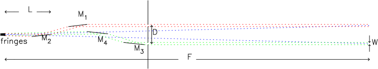
Figure 2: The four flat mirror configuration. The diagram is not drawn to scale. The axial distance between $M_{2}$ and $M_{3}$ is much less than the distance L and $F$ is much larger than $L$. The vertical scale is exaggerated so that the beam widths are visible.

All four mirrors are set at grazing incidence to provide high reflectivity. Operating in the soft X-ray band 0.1-2.0 keV the grazing angles need to be $\theta_{g}\approx 2^{\circ}$. If $M_{1}$ and $M_{3}$ are set at $\theta_{g}$ with respect to the x-axis then $M_{2}$ and $M_{4}$ must be set at a slightly smaller angle $\theta_{g}-\theta_{b}/4$ so that the beams overlap to form fringes. Since $\theta_{b}$ is very small compared to $\theta_{g}$, $M_{2}$ is almost parallel to $M_{1}$ and the same is true for $M_{4}$ and $M_{3}$. The effective focal length $F$ is much larger than $L$ and is given by $\phi=\theta_{b}/2=\tan^{-1}(R/F)$. The fringe spacing is then $\Delta y=F\delta\theta=F\lambda/D$ where $\Delta\theta$ is the diffraction limited angular resolution for the baseline separation $D$ operating at wavelength $\lambda$.

The arrangement is similar to that used by Cash et al. [3] but the front of $M_{2}$ is placed at distance $L$ from the maximum overlap of the beams whereas in the Cash configuration this mirror is at a distance $2L$ from the maximum overlap. The present configuration reduces the overall length required by a useful factor of two. The physical length of the system is much smaller than the focal length as is the case for a Wolter II telescope. If $W=300$ $\mu$m (see above) then the axial length of the mirrors is only 8.6 mm if $\theta_{g}=2^{\circ}$. The axial distance covered by the combination of $M_{1}$ and $M_{4}$ need only be $\sim 25$ mm. The axial distance between $M_{1}$ and $M_{2}$ (or $M_{3}$ and $M_{4}$) is $D/(4\tan\theta_{g})\approx 7D$.

4.1 A slatted mirror

The collecting area afforded by a single four mirror arrangement as illustrated in Fig. 2 is going to be small for any sensible depth of mirror (along the z-axis into the plane of the paper). Furthermore the mirrors required would be incredibly long and thin because the axial length utilised is so small (8.6 mm, see above). A major advantage of the four mirror configuration proposed here and illustrated in Fig. 2 is that a series of parallel systems can be stacked together. In order to do this the axial length of mirrors $M_{1}$, $M_{3}$ and $M_{4}$ must be extended thereby increasing the aperture widths and the mirror $M_{2}$ must be split into a slatted mirror as shown in Fig. 3.

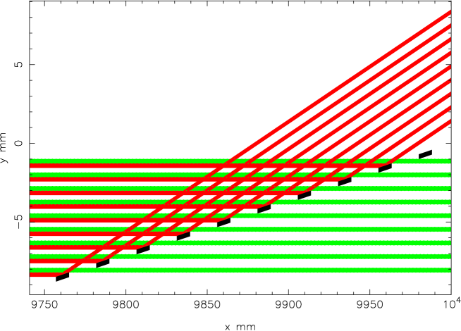
Figure 3: The beam paths using a slatted mirror

Each slat is a long thin mirror facet extending into the plane of the paper. The axial width of a slat is the same as for the mirrors in Fig. 2. The slats are spaced so that the beam from mirror $M_{4}$, to the right, is broken into a series of beams of width $W$. Each slat mirror reflects a fraction of the beam from mirror $M_{1}$ creating a second set of beams. Each pair of beams overlap to form interference fringes. Providing there is not too much blocking from support structure needed to hold the slatted mirror together and provided the thickness of the mirror slats is the same order as the beam width $W$ then about one third of the flux collected by the apertures of $M_{1}$ and $M_{3}$ will form fringes. A slatted mirror with $\sim 30$ slats will provide an effective aperture width of $\sim 1$ cm. The axial length for each slat-gap pair will be $\sim 26$ mm. Fig. 4 is a schematic diagram of the layout using a slatted mirror with 30 elements. The length $\Delta L$ is the axial separation of $M_{1}$ and $M_{4}$ and the baseline separation $D$ is the same for all the slat-gap pairs.

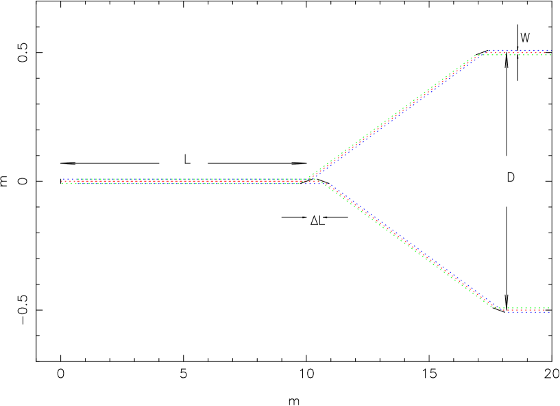
Figure 4: The layout of an X-ray interferometer using a slatted mirror with 30 elements. Note that the vertical scale is expanded so that the geometry of the beams is easier to discern.

Such a slatted mirror is like a macroscopic transmission grating with mirror facets on each line. It is likely that an optical element of this form could be manufactured using similar techniques to those currently employed in the fabrication of X-ray transmission or reflection gratings. A slatted mirror with dimensions $500\times 500$ mm combined with 3 plane mirrors of the same size would provide a total collecting area $\sim 50$ cm².

4.2 Path lengths

If the mirrors in each arm are set parallel the path length from the aperture at $M_{3}$ to the detector plane is

$$P_{0}=(L+\Delta L+\frac{D}{2\cos 2\theta_{g}})(\frac{1}{\cos\theta}-1)\approx(L+\Delta L+\frac{D}{2\cos 2\theta_{g}})\frac{\theta^{2}}{2}$$ (6)

where $\theta$ is the off-axis angle of the source. This is the same for both arms $M_{1}$-$M_{2}$ and $M_{3}$-$M_{4}$ and for all positions across the detector. When $M_{2}$ and $M_{4}$ are tilted by $\theta_{b}/4$ to produce an overlap between the beams we get an extra path contribution. The extra path lengths of the two arms are then:

$$P_{12}=L(\frac{1}{\cos(\theta_{b}/2)}-1)+y\sin(\theta_{b}/2)-\frac{D}{2}\sin\theta$$ (7)

$$P_{34}=(L+\Delta L)(\frac{1}{\cos(\theta_{b}/2)}-1)-y\sin(\theta_{b}/2)+\frac{D}{2}\sin\theta$$ (8)

where y is the position across the detector plane. The path difference between the arms is:

$$\Delta=P_{12}-P_{34}=-\Delta L(\frac{1}{\cos(\theta_{b}/2)}-1)+2y\sin(\theta_{b}/2)+D\sin\theta$$ (9)

It is this path difference which give rise to the fringes. The first term is fixed and of no consequence since it can be eliminated by a small change in the position of $M_{1}$ or $M_{3}$. Ignoring this small correction the coincidence point of the interferemeter ($\Delta=0$) is given by

$$y=\frac{-D\sin\theta}{2\sin(\theta_{b}/2)}\approx-F\theta$$ (10)

Here we have taken the small angle approximation and substituted for the focal length $F=R/\tan(\theta_{b}/2)\approx D/\theta_{b}$. The interferometer behaves like a telescope of focal length $F$ with the coincidence point (centre of the fringe pattern) at the expected position of a point source with off-axis angle $\theta$. The negative sign represents the expected lateral inversion in the focal plane.

4.3 The fringe pattern

If we move away from the coincidence point the path difference $\Delta$ increases linearly with $y^{\prime}=y+F\theta$ and we expect to observe cosine fringes. Because the wavefronts of the two beams are broken up by the slatted mirror we must use Fresnel diffraction theory to calculate the exact form of the fringe pattern. If plane waves of wavelength $\lambda$ are incident on a slit of width $W$ and we are looking at the fringes at a distance $L$ from the slit the dimensionless variable used in the Fresnel integrals is given by

$$u=y^{\prime}\sqrt{\frac{2}{\lambda L}}$$ (11)

Substituting for $y^{\prime}=W$ from equation 5 we have $u_{0}=\sqrt{2N_{f}}$. Since $N_{f}>1$ the scaled width of the slit $u_{0}$ is also $>1$ and we must use the near field approximation (Fresnel diffraction) rather than the far field limit (Fraunhofer diffraction).

We define limits $u_{1}=u-u_{0}/2$ and $u_{2}=u+u_{0}/2$. The complex amplitude at a scaled displacement $u$ from the centre of the beam is given by

$$A=C(u_{2})-C(u_{1})+i(S(u_{2})-S(u_{1}))$$ (12)

where $C(u)$ and $S(u)$ are the Fresnel integrals

$$C(u)=\int_{0}^{u}\cos(\pi w^{2}/2)dw$$ (13)

$$S(u)=\int_{0}^{u}\sin(\pi w^{2}/2)dw$$ (14)

The intensity expected is then given by $I=AA^{*}$. Using the beam parameters from above $u_{0}=4.5$ and the intensity has the profile shown in the left-hand panel of Fig. 5. The geometric shadow of the edges of the slit (a mirror slat or gap between slats) without diffraction are expected at $u=\pm 2.25$.

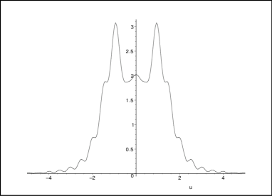
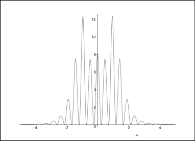
Figure 5: Left panel: The Fresnel diffraction profile of a single beam. Right panel: The fringe pattern from one slat-gap pair.

If the mirror slats and gaps are the same size they will produce identical intensity profiles but because they are tilted by $\theta_{b}$ with respect to each other there is a phase difference between the beams which is a linear function of $u$, $\delta=\pi u_{0}u$, and the complex amplitude in the overlap region is then given by

$$A_{2}=A(1+\exp(i\pi u_{0}u))$$ (15)

Again we can calculate the intensity profile in the same way giving the fringe pattern plotted in right-hand panel of Fig. 5. The intensity of the bright fringes is modulated by the Fresnel diffraction profile shown in the left-hand panel of Fig. 5. The expected $N_{f}=10$ fringes are visible across the centre of the beam. The edges of the beam spread into the geometric shadow due to diffraction but there should be negligible interference between adjacent slat-gap pairs.

As the path difference $\Delta$ becomes comparable to the coherence length of the X-rays the visibility of the fringes will decrease. If $E/\Delta E=N$ then we expect to see $\sim N$ fringes across the entire pattern. If $N>>N_{f}$ then a continuation of the fringes will be visible from slat-gap pairs adjacent to the coincidence position. However only $\sim$half the fringes will be detected because of the gaps. These missing fringes can be recovered by splitting the slatted mirror into two halves, reversing the slat and gap positions in the second half. The pattern of slats required is shown in Fig. 6. Combining the fringe patterns from the two halves provides complete coverage of all $N$ fringes. Fig. 7 shows the fringe pattern expected from two sources at $\pm 5$ mas with $N_{f}\sim 4$ and $N\sim 10$. The slats introduce a residual modulation but this can be completely removed during analysis of the interferograms.

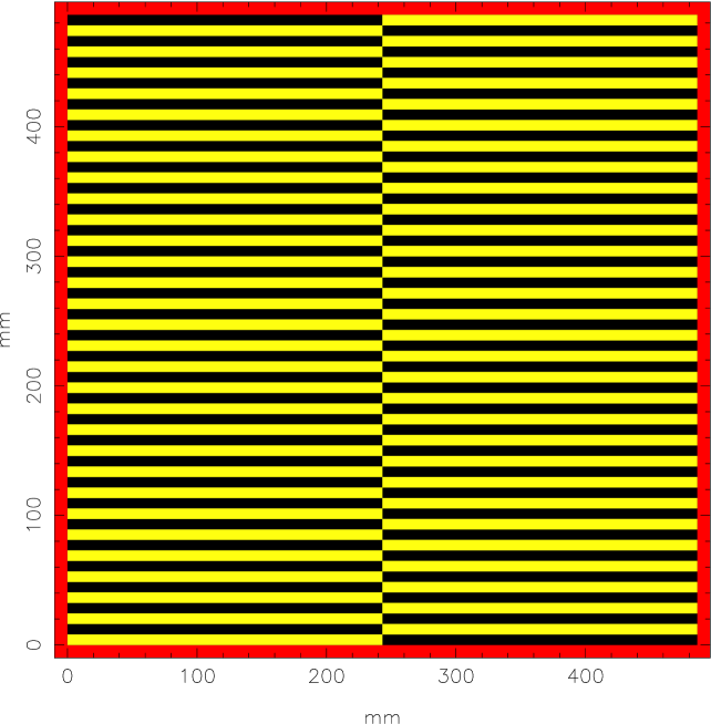
Figure 6: A slatted mirror with complementary halves.

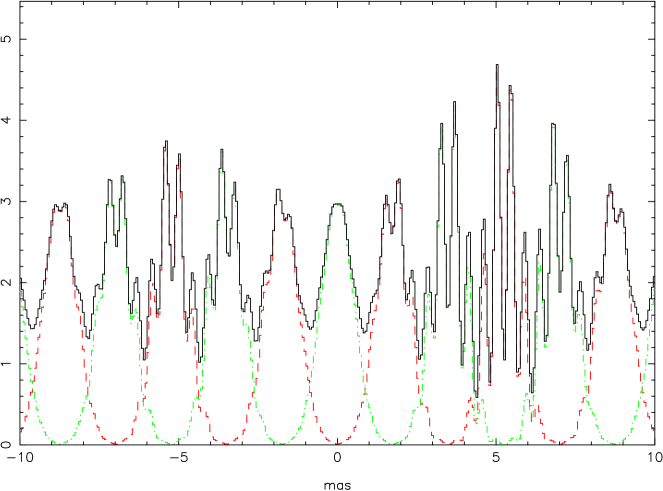
Figure 7: The fringe pattern expected from 2 sources at $\pm 5$ mas. The fringes from the two halves of the slatted mirror are plotted as dash and dash-dot lines.

4.4 Detecting the fringe pattern

Working at an X-ray wavelength of $10$ Å and using $L=10$ m the fringe spacing for $N_{f}=10$ is $30$ $\mu$m. Such fringes could be resolved using a CCD detector with the smaller pixel sizes currently available. However the fringes exist through a very long volume in which the two beams overlap. All 10 fringes should be visible over an axial depth of $\sim L/10$. If the detector is set at a grazing angle $\theta_{d}$ to the beam the fringe spacing will be increased to

$$\Delta y^{\prime}=\frac{\Delta y}{\sin\theta_{d}}$$ (16)

If $\theta_{d}=5.7^{\circ}$ then the magnification factor will be 10 and the fringes will easily be resolved by current detector technology. Unfortunately a detector operating at such a low grazing angle will have a low efficiency. In order to take advantage of the magnification a detector with high quantum efficiency operating at small grazing angles would have to be developed.

When observing astronomical objects the X-ray flux will be broadband and a detector with a moderate energy resolution will be required to detect fringes. We require an energy resolution $E/\Delta E\geq N_{f}$ to resolve the fringes at energy $E$ in a bandwidth $\Delta E$. A CCD typically has $E/\Delta E\approx 10$ at 0.6 keV increasing to $\sim 15$ at 1 keV and $\sim 50$ at 7 keV. This is just adequate for our purpose. However, the imaging and spectral response of a CCD is not well matched to the requirement. High spatial resolution is only needed in 1-D (across the fringes) and the sensitivity would be greatly improved if $E/\Delta E>100$.

4.5 Simulation of one-dimensional imaging

The interferometer illustrated in Fig. 4 has been simulated using the slatted mirror layout shown in Fig. 6 and the energy response of the XMM-Newton EPIC-MOS CCDs [7]. In order to get good coverage on the u-axis (spatial frequency) four parallel systems were used with D-spacings of 35, 105, 315 and 945 mm. The corresponding effective focal lengths are 1.2, 3.7, 11.1 and 33.4 km. Each system has a collecting area of $\sim 20$ cm² in the energy band 0.58-2.1 keV (using the reflectivity of gold and the MOS detector efficiency). The $E/\Delta E$ of the detector provides 21 energy channels across this band. A total source flux equivalent to 1 Crab gives 460000 counts in a 1000 second exposure. With 4 D-spacings and 21 energy channels a total of 84 interferograms were recorded in a single exposure. The source distribution assumed was a binary system consisting of an extended source and a point-like companion.

Even with $\sim 460000$ counts the count per fringe is very small and it is impossible to see the fringes in the raw simulated data. However, for each interferogram (1 energy channel and 1 D-spacing) the fringe spacing and expected number of fringes is known. It is therefore possible to set up a Fourier filter that picks out the fringe pattern from each interferogram. Fig. 8 shows the Fourier power spectra of the 84 interferograms and the Fourier filter constructed to pick out the fringes. The 4 blocks of 21 interferograms arise from the 4 D-spacings used.

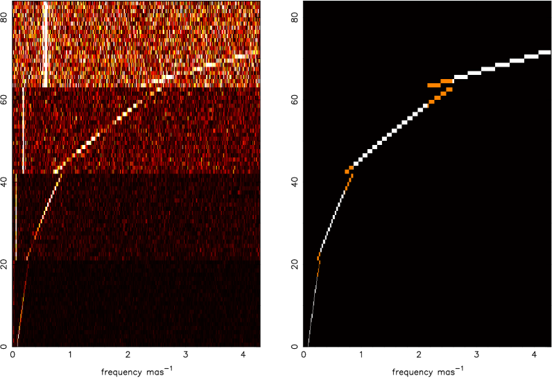
Figure 8: The left-hand panel shows the Fourier power spectra of 84 interferograms. Each block of 21 corresponds to a given D-spacing. The right-hand panel is the Fourier filter used to pick out the fringes.

Two peaks are visible in each power spectrum. The vertical white lines to the left at low frequency are the peaks from the modulation caused by the slats. These are completely removed by the filtering. The white patches to the right are the fringes. The visibility of the fringes varies as the frequency increases because of the structure of the binary source under observation. A top-hat profile matched to the $E/\Delta E$ for each interferogram was used to construct the filter. There is some overlap in the frequency coverage between the 4 D-spacings. In a practical set up the overlap regions could provide a means of eliminating phase errors between the 4 parallel optical systems. Fig. 9 shows the reconstruction of the source distribution.

Figure 9: The reconstructed source distribution. The inset shows an expanded detail of the significant peaks. The binary consists of a resolved component with a point source companion.

The intensity is plotted as counts per 0.058 mas sample and there are 1800 samples across the field of view. The rms noise level is 2.16 counts per sample and all the significant samples are detected at $>12\sigma$. The total estimated count from the significant samples is 430000 compared with the actual detected count of 462000 so 93% of the original count has been successfully imaged.

In this simulation and reconstruction the source distribution was assumed to be independent of energy and therefore all the detector energy channels could be summed to produce the final image. In reality this would not always be the case and more D-spacings would be required to reconstruct a source with a complex spatial-energy structure. To extend the imaging to 2-D more exposures would be required at different roll angles about the pointing axis to give a reasonable coverage in the (u,v) plane. If this were achieved by running several (5-10) identical systems simultaneously at different roll angles not only would 2-D imaging be provided but there would also be a pro rata increase in the total collecting area.

The system performs in a similar way to a shadow mask camera [6] but a fringe pattern is detected instead of a shadow mask pattern. Each pixel at the detector is multiplexed to many sky elements within the field of view and therefore the sensitivity of the interferometer is dependant on the source distribution or the number of significantly bright point sources in the field of view. If the energy resolution of the detector were improved the number of fringes $N\approx E/\Delta E$ across the pattern would increase and the number of pixels multiplexed to a given sky position would be larger. The total area of the Fourier plane covered by the filter (Fig. 8) is $\propto 1/N$ and if there are $N_{x}$ significant unresolved sources in the field-of-view the signal-to-noise is $\propto\sqrt{(}N)/N_{x}$.

5 Tolerances, alignment and adjustment

In the practical implementation of the interferometer we must consider:

• figure errors in the flat mirror surfaces

• roughness of the mirror surfaces

• angular alignment of the mirrors

• positional placement of the mirrors

• control of the difference between the path lengths in the two beams

• pointing accuracy and stability

5.1 Figure errors and surface roughness

The mirrors must be flat enough so that incident plane wavefronts are reflected with the minimum perturbation and remain plane. Figure errors will introduce distortions in the wavefronts and shorter scale surface roughness features will scatter some of the incident light into scattering wings which will reduce the contrast of the fringes. Fortunately, because the mirrors are operating at grazing incidence, the effect of figure errors and surface roughness in the mirror surfaces is reduced by a factor $\sin\theta_{g}$. A surface height error $h$ introduces a wavefront shift of $2h\sin\theta_{g}$. To produce clean fringes the wavefronts must not be perturbed by greater than $\sim\lambda/10$. So we have

$$h\leq\frac{\lambda}{20\sin\theta_{g}}$$ (17)

If $\lambda=10$ Å and $\theta_{g}=3^{\circ}$ then we require $h<1$ nm. A high quality optical flat has a specification of $\lambda/20$ (where $\lambda=633$ nm) so even with the advantage of grazing incidence we need very high quality mirrors to obtain clean fringes. The surface height error of 1 nm is equivalent to an axial gradient error over the width of 1 slat of $\sim 0.03$ arc seconds. Gradient errors over distances larger than the slat width will destroy the register between the overlapping beams produced by a single slat-gap pair and may introduce confusion between adjacent slat-gap pairs. The angular width of the fringe separation is $\Delta y/L\approx 3\times 10^{-6}$ equivalent to 0.6 arc seconds as seen from the mirrors. Therefore gradient errors between the slats and over the full faces of the other mirrors must be kept to this level.

First order perturbation theory gives the Total Integrated Scatter (TIS) after two reflections as

$$TIS=2(\frac{4\pi\sigma\sin\theta_{g}}{\lambda})^{2}$$ (18)

where $\sigma$ is the rms surface roughness. To get $TIS<0.1$ we require $\sigma<3.5$ Å integrated over correlation lengths $<1$ mm on the surface.

The quality of mirror surfaces required is high, similar to the best X-ray mirrors used in instruments such as Chandra. However the surfaces are flat rather than aspherics and therefore they should be significantly easier to manufacture than Wolter type I surfaces. Manufacture of the slatted mirror imposes a much higher level of difficulty since the mirror surfaces must be flat but the substrate must be very thin and extra support will be required to hold the slats together without introducing too much blocking of the aperture.

5.2 Adjustment and stability of the D-spacing

The baseline separation $D$ is set by the distances $d_{12}$ and $d_{34}$ measured between the mirror centres, $D=(d_{12}+d_{34})/\sin 2\theta_{g}$. These distances can be reduced until a minimum $D_{min}=4WN_{s}$ where $N_{s}$ is the number of slats in mirror 2. If the mirrors are brought any closer than this the outer edges of the mirrors 2 and 4 will start to be blocked and fringes will only be seen for the central slat-gap pairs in mirror 2. $D_{min}$ is the minimum baseline for which the full collecting area is available.

The distances $d_{12}$ and $d_{34}$ must be the same so that the path lengths for the two beams are identical. To change the baseline both mirrors 1 and 3 must be moved. An off-axis angle of $\theta$ introduces a path difference $\Delta=D\sin\theta$ (see equation 9). Thus adjustments of $d_{12}$ and $d_{34}$ are coupled to the pointing direction $\theta$. If you imagine that mirror 3 is fixed at position $d_{34}$ and rotation $\theta_{3}$ then the path lengths can then be equalized either by adjusting $d_{12}$ or by changing the pointing $\theta$. Of course this coupling is why the phase and visibility of the fringes observed give us information on the angular distribution of the source.

The total path difference between the two beams must be less than the coherence length of the X-rays or the fringes will disappear. A coherence length of 10 $\mu$m corresponds to a wave train of 10000 cycles but this order of coherence will only be seen in line radiation for which the radiative lifetime is relatively large. In astronomical observations the source spectrum is dominated by continuum radiation and the effective coherence length will be determined by the energy resolution of the detector system. Using CCD technology at $\sim 1$ keV the wave trains will be just 10 cycles long. In this case we must control $d_{12}-d_{34}$ to order 10 nm or set $\theta<10\lambda/D$. If $D=10$ mm then $\theta<0.2$ arc seconds.

6 Conclusion

We have described the design of an X-ray interferometer that can fit into a tube $\sim 20$ m long and $\sim 2$ m diameter. The simplest configuration which can provide full 1-D imaging consists of 4 optical units. Each unit comprises 3 flat mirrors, a flat slatted mirror and an array of CCD detectors. The combination gives a collecting area of $\sim 80$ cm² in the energy band 0.58-2.1 keV and an angular resolution of $\sim 0.1$ mas over a field of view 100 mas across. A simple field of view containing $N_{x}\approx 10$ significant unresolved sources with a total flux equivalent to 1 Crab can be imaged to a sensitivity $>5\sigma$ in 500 seconds. The system can provide imaging in 2-D by making exposures at different roll angles. About 40 units (possibly packed into the same tube) running simultaneously with different D-spacings and roll angles could provide good coverage of the (u,v) plane and because of the 10-fold increase in collecting area the same sensitivity would be achieved in $\sim 150$ seconds using CCDs or detectors with a similar performance. If the detector energy resolution could be improved by a factor of 10 while retaining a spatial resolution of $\sim 10\mu$ m in 1-D then the same 2-D imaging sensitivity could be achieved in $\sim 50$ seconds.

The interferometer requires a high quality slatted mirror the specifications of which are challenging but probably well within current manufacturing capability. However, such a mirror has not been produced and needs to be developed.

The system is similar to the MAXIM periscope configuration, the tolerances of which are described by Shipley et al. [8]. An equivalent study of the tolerances and tradeoffs is required for the present concept to further the design of the optical bench needed.

The introduction of a slatted mirror dramatically reduces the total distance required between the primary mirrors that define the baseline separation and the detector system and 0.1 mas imaging can be achieved without the requirement for two free-flying spacecraft as considered for the MAXIM Pathfinder [9] or the many free flying spacecraft required for the all-up MAXIM configuration [10]. Each unit of 4 mirrors detects two-source fringes and the combination of several such units provides imaging by aperture synthesis in the same way as conventional interferometers used in the radio and optical bands. This is rather different from the all-up MAXIM approach in which many mirror segments are used to produce a complex interferogram which is much closer to a conventional image. As a first step towards ultra high angular resolution X-ray astronomy the present scheme is more compact and easier to implement than the MAXIM configurations considered thus far.

References

- [1] Baldwin, J.E. et al., 1996, Astron. Astrophys. 306, L13-L16
- [2] Monnier, J.D., 2003, Rep. Prog. Phys. 66,789-857
- [3] Cash, W., Shipley, A., Osterman, S. and Marshall, J., 2000, Nature vol. 407, 160
- [4] Suzuki, Y., 2004, Rev.Sci.Instrum., Vol. 75, No. 4., 1026-1029
- [5] Weisskopf, M.C., O’Dell, S.L., VanSpeybroeck, L.P., 1996, Advanced X-ray Astrophysics Facility (AXAF): An overview. Proc. Soc. Photo-Opt. Eng. 2805, 2-7
- [6] Sims M.R., Turner M.J.L., Willingale R., Nucl. Instr. & Meth, in Phys. Res. 228, 512, 1980
- [7] Turner M.J.L. et al., 2001, A&A, 365, L27-L35
- [8] Shipley A., Cash W.C., Gendreau K., Gallagher D., 2003, SPIE Vol. 4851, 568-576
- [9] Gendreau K.C., Cash W.C., Shipley A.F., White N., 2003, SPIE Vol. 4851, 353-363
- [10] Lieber M., Gallagher D., Cash W., Shipley A., 2003, SPIE Vol. 4851, 557-567