The dwarf galaxy population in Abell 2218

Abstract

We present results from a deep photometric study of the rich galaxy cluster Abell 2218 ($z=0.18$) based on archival HST WFPC2 F606W images. These have been used to derive the luminosity function to extremely faint limits ($M_{\rm F606W}\approx-13.2$ mag, $\mu_{0}\approx 24.7$ mag arcsec^-2) over a wide field of view ($1.3\;h^{-2}\;$Mpc²). We find the faint-end slope of the luminosity function to vary with environment within the cluster, going from $\alpha=-1.23\pm 0.13$ within the projected central core of the cluster ($100<r<300\,h^{-1}$ kpc) to $\alpha=-1.49\pm 0.06$ outside this radius ($300<r<750\,h^{-1}$ kpc). We infer that the core is ’dwarf depleted’, and further quantify this by studying the ratio of ‘dwarf’ to ‘giant’ galaxies and its dependency as a function of cluster-centric radius and local galaxy density. We find that this ratio varies strongly with both quantities, and that the dwarf galaxy population in A2218 has a more extended distribution than the giant galaxy population.

1 Introduction

The galaxy luminosity function (LF) – the number density of galaxies per unit luminosity interval – is a fundamental descriptor of the galaxy population and, as such, contains important information on the formation and evolution of galaxies (Bingelli, Sandage & Tammann 1988, Benson et al. 2003). At low redshift, the LF will contain the combined imprints of the galaxy initial mass function (Press & Schechter 1974, Schechter 1976), together with the effects of any subsequent evolutionary processes which modified this distribution (e.g., hierarchical merging; White & Rees 1978). Determinations of the LF in different environments and at a variety of redshifts provide the only direct hope of disentangling these environmental and evolutionary effects.

In this context, rich clusters are fundamental testing grounds, representing the densest environments in which galaxies reside and, within the hierarchical clustering framework, the ultimate examples of where build-up through merging has taken place. Here galaxies at all luminosities, both bright and faint, may bear evidence of environmental effects: the ‘giant’ ($L>L^{*}$) galaxies at the bright end of the LF are the strongest candidates for having been built up through successive mergers and accretion (e.g. Kauffmann, White & Guiderdoni 1993). Equally, the sub-luminous ($L<L^{*}$) ‘dwarf’ galaxy population may be a victim of, and therefore depleted by, these merging and cannibalisation processes. In contrast, galaxy ‘harassment’ may boost the dwarf galaxy population through whittling down more luminous cluster galaxies as they undergo high speed encounters (Moore et al. 1996). Additionally, both giant and dwarf galaxies in the core regions of clusters are likely to be susceptible to such processes as ram-pressure stripping (Gunn & Gott 1972) and cluster tidal effects (Byrd & Valtonen 1990, Bekki et al. 2001), which severely modify their star forming activity and hence their luminosity (see also Bower & Balogh 2003, Moore 2003).

This potential for the rich cluster LF to be used as an evolutionary ‘probe’ has led to numerous efforts to measure it. In recent times, the faint-end slope of the LF – described by the parameter, $\alpha$, in the Schechter (1976) function representation – has been of particular focus, with numerous claims that it is significantly steeper in clusters than in the general field (De Propris & Pritchet 1998, Trentham & Tully 2002).

Comparison of cluster LF results is, however, complicated by a number of factors: the differing magnitude ranges over which the slope is calculated, the different methods of field galaxy subtraction employed by different authors, and the different physical cluster cross-sections covered (Driver & De Propris 2003). A further complication is that some observations suggest the numbers of dwarf galaxies varies with environment – what Phillipps et al. (1998) referred to as a “dwarf population–density” relation. This manifests itself as the densest regions in clusters having the lowest dwarf galaxy fractions, the ratio of dwarf to giant galaxies increasing with decreasing giant galaxy density, and the dwarf populations in clusters being more spatially extended than the giants (Smith et al. 1997, Driver et al. 1998a, Driver et al. 2003). This is also compounded by the likelihood that there exist two dwarf populations, such as seen in Virgo, whereby the dwarf ellipticals are centrally concentrated (e.g., Binggeli, Sandage & Tammann 1985; Conselice et al. 2003) and the dwarf irregulars (and/or dwarf low surface brightness galaxies) lie predominantly in the halo (Sabatini et al. 2003).

In this paper we present a case study of the well known rich cluster Abell (A)2218 at $z=0.18$, deriving its LF to very faint limits and over a broad range of environment from deep, wide-field imaging obtained with the Hubble Space Telescope (HST). Famous for its spectacular strong gravitational lensing of background galaxies (Kneib et al. 1996), A2218 is an Abell richness class 4 cluster with a Bautz Morgan type of II, whose centre is dominated by a large, low surface brightness cD galaxy with an envelope extending over more than 180h^-1 kpc (Pello-Descayre et al. 1988). It also has a massive, deep potential well, with a central velocity dispersion of 1370 km s^-1 (Le Borgne et al. 1992), and is a strong X-ray emitter [$L_{X}$(0.5–4.4 keV)$=3.3\times 10^{44}\,h_{100}^{-2}$ erg s^-1; Jones et al. 1993]. Moreover, a strong Sunyaev-Zeldovich decrement is observed in its direction (Birkinshaw & Hughes 1994). As well as providing an extreme case in the context of observing environmental effects, A2218 is also a propitious choice in that its high richness makes it particularly amenable to reliable ‘background’ removal using statistical methods (Driver et al. 1998b).

The layout of this paper is as follows: In section 2 we describe the HST imaging of A2218, and the procedures followed in the detection and photometry of objects, star/galaxy separation, and the extraction of the cluster population through the careful subtraction of the background population. For the latter, considerable attention is paid to the numerous effects that contribute uncertainties to this process, in particular the effect of gravitational lensing. In section 3 we present the luminosity function, subdivided into inner (projected core) and outer (halo) components. We then determine the dwarf-to-giant ratio versus giant galaxy density and investigate the radial profiles of the giant, dwarf and ultra-dwarf galaxies (defined below). We summarise and discuss our results in section 4. Throughout we adopt a ${\Omega}_{\rm M}=0.3$, ${\Omega}_{\Lambda}=0.7$ and $H_{0}=100{\rm kms^{-1}Mpc^{-1}}$ cosmology; this puts A2218 at a distance modulus of $39.01$ mag (inclusive of a $k$-correction), with 1 arcmin projecting to 128 co-moving kpc at this distance.

2 Data Analysis

Our study is based on archival HST Wide Field Planetary Camera 2 (WFPC2) images of A2218, obtained as part of a program to study weak gravitational lensing (PI: Squires, PID:7343) over a much larger region of this cluster than that covered in the original strong-lensing study (Kneib et al. 1995). These data comprise a mosaic of 22 pointings in the F606W passband. Each pointing involved a total exposure time of 8,400 s. The location of these pointings on the sky is shown in Figure 1; the mosaic provides coverage of a roughly square field with a total area of $\approx 82\;{\rm arcmin}^{2}$. The resolution, depth and coverage of the data are unique and particularly well suited to investigating A2218’s galaxy population down to very faint limits and out to a radius of $\sim 0.75\,h^{-1}$Mpc from its centre.

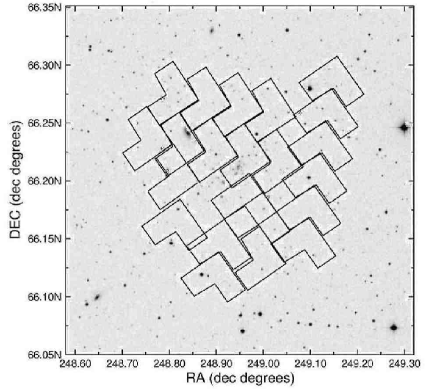
Figure 1: The HST WFPC2 mosaic used for this study, showing the arrangement and location of the 22 pointings on the sky. A total exposure time of 8,400 s was obtained at each pointing. This is overlayed on top of a digital sky survey image of the A2218 field.

The HST data were obtained from the HST archive with the standard procedures of bias removal and flat-field division having been applied. Each pointing consists of 12 dithered exposures, each of 700 s duration. In order to remove cosmic rays, the individual frames were drizzled together using the drizzle task in the IRAF dither package, following the procedure of Koekemoer et al. (2002). The final drizzled image had a pixel size of 0.0498 arcsec. Only the portions of each pointing with the full 8,400 s of exposure were used in the analysis, resulting in a final overall field-of-view of 0.0228 sq. degrees or 1.34 Mpc² at the cluster redshift. The photometric zero point adopted for our data was that published for the WFPC2 by Holtzman et al. (1995), which places the instrumental F606W magnitudes onto the VEGA system. The quoted accuracy of this zeropoint is 2%.

2.1 Object detection and photometry

Objects were detected and photometered using the SExtractor package of Bertin & Arnouts (1996). Based on previous experience in using SExtractor with WFPC2 images, a detection criterion of 20 connected pixels 1.5$\sigma$ above the sky RMS was used. Figure 2 shows a typical image obtained with one of the WFPC2 CCDs (WF3), with the objects detected by SExtractor circled. The magnitude best_mag was used as our measure of total galaxy magnitude (hereafter denoted simply as $F606W$). This adopts a Kron magnitude as the default value, except for crowded regions where an extrapolated isophotal magnitude is used. Note that radius of the Kron (1980) extraction aperture is set to 2.5 times $R_{k}$ where $R_{k}$ is the first moment of the image distribution. A total of 8038 objects were detected with $F606W\leq 25.8$ mag (equivalent to $M_{\rm F606W}\leq-13.2$ mag), the magnitude at which the number of detections turned over.

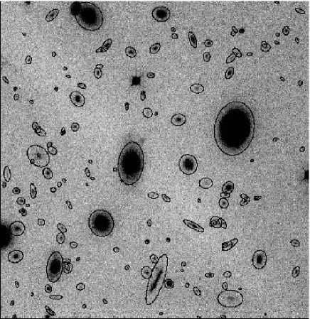
Figure 2: A typical image obtained with one of the WFPC2 CCDs (WF3) with SExtractor detections circled. The image is $80^{\prime\prime}$ ($0.17\,h^{-1}$ Mpc) on a side.

The SExtractor parameter class_star was used as the basis for separating stars from galaxies, supplemented by visual inspection in the small number of cases where the software was equivocal in its classification.

A broad overview of the range and depth of the objects detected by SExtractor and in particular the population of galaxies included in this study, is shown in Figure 3. Here we plot the mean central surface brightness, $\mu_{\rm app}$ (measured in a circular aperture of area equivalent to the 20-pixel minimum required for object detection), of all our detected objects as a function of their apparent total magnitude. This reveals three distinct populations of object: cosmic rays, which form the tight upper-most diagonal locus, stars, which form the slightly broader central locus, and galaxies, which form the lower-most broad wedge of objects. The stars and galaxies are clearly distinguishable down to $F606W\sim 24$. Also of note is the surface-brightness ‘edge’ to the galaxy population, with no objects seen fainter than $\mu_{\rm app}\sim 24.5$ mag arcsec². This is consistent with the $1.5\sigma$ isophotal detection limit used in SExtractor, which corresponds to $\mu\approx 24.7$ mag arcsec^-2. Given the way the galaxy wedge broadens with increasing magnitude and surface brightness, it is clear that our sampling of the galaxy population is surface-brightness limited at magnitudes fainter than $F606W\sim 23$. However, as we discuss in the following section, this has little impact on our ability to accurately quantify the cluster galaxy counts at these faint apparent magnitudes.

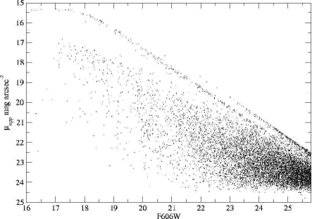
Figure 3: The aperture surface brightness of all our detected objects, plotted as a function of apparent magnitude. The measured objects, represented by the dots, are clearly seen to define three distinct loci within this diagram: cosmic-rays (upper-most locus), stars (central locus), and galaxies (lower wedge). Stars and galaxies are easily separated down to a magnitude of $F606W\sim 24.5$.

2.2 Field galaxy removal

In the absence of spectroscopy, the removal of the foreground and background ’field’ galaxy populations must be done statistically. Here we follow the strategy adopted by Driver et al. (2003) for a similar HST-based study of the rich cluster Abell 868 ($z=0.15$). This involved estimating the field galaxy counts from the deepest available HST/WFPC2 data taken in the F606W band. This comprised images of the Hubble Deep Field (HDF) North (Williams et al. 1996), the HDF-South (Casertano et al. 2000), and 10 other fields with total exposure times between 10,000–20,000 s (and hence of comparable depth to our A2218 cluster mosaic). Object detection and photometry was performed on these images using SExtractor, with an identical set of parameters to those used on our A2218 data.

The galaxy number counts derived from these data are shown in Figure 4, where we have plotted the combined counts from the two HDF fields and those from the 10 other reference fields separately. To within the uncertainties, we see that there is no significant difference in the galaxy counts between the ‘deep’ (HDF) and ‘shallow’ reference fields. This is important, since by including the much deeper HDF data (surface brightness limit of $\mu_{\rm app}\sim 26.0$ mag arcsec² cf. limit of $\mu_{\rm app}\sim 24.5$ mag arcsec² for our ‘shallow’ reference fields and A2218 – see Fig. 3) in our field galaxy count estimates, we want to be certain that this does not lead to an over-estimation through the inclusion of an additional population of faint, low surface brightness galaxies unseen in our cluster images. The agreement seen between the two different sets of number counts shown in Figure 4 would indicate this is not the case. Hence we can be confident that our selection limits are identical both inside and outside the cluster, and the excess galaxy counts we observe after field subtraction is due to having detected a bona fide population of cluster galaxies rather than one that is spurious.

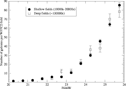
Figure 4: The combined HDF-North and HDF-South galaxy counts (open squares) and the combined shallower reference counts (closed circles), plotted on a linear scale to aid comparison. The consistency of the counts implies negligible selection bias in either the detection or photometry between the shallow and deep fields.

In the top panel of Figure 5 we plot in the traditional way, the galaxy number counts for both the ’field’ (as per Figure 4) and what we measure in the direction of A2218. We also supplement the counts at bright magnitudes ($F606W\leq 17.5$) by plotting those derived from the ground-based Millennium Galaxy Catalog (MGC) by Liske et al. (2003). We caution that this has involved transforming the MGC counts from the $B$-band (in which they were measured) onto our $F606W$(VEGA) system. This we did using the relation $B_{\rm MGC}-F606W$(VEGA)$=1.06$ derived by Driver et al 2003. This simple colour conversion is only strictly valid for the very bright end of the MGC counts: $F606W<17.5$ mag. However, since their only purpose in this study is to provide a bright magnitude ‘anchor’ point – the accuracy of which has a negligible effect on the overall accuracy of our field galaxy subtraction at the much more critical fainter magnitudes – this is quite satisfactory.

Comparison of the A2218 and field counts in the upper panel of Figure 5 shows a clear divergence between the two with decreasing magnitude, with the field counts having a slope close to the canonical value of $\sim 0.4$ observed in other studies at these wavelengths (e.g., Metcalfe et al. 2001). To provide a clearer picture of the deviation between the A2218 and field counts, we plot in the lower panel of Figure 5 the counts relative to the $N\propto 10^{0.4\,m}$ relation (where $m$ represents our F606W magnitudes), appropriately normalised to the A2218 mosaic field of view. This reveals some residual magnitude dependence in the field counts, so to account for this and ensure that they are accurately represented over the entire magnitude range covered by our study, we fit a quadratic to the combined MGC+WFPC2 counts, yielding:

$${d\log_{10}N\over dm}=-12.9346+0.96077m-0.012874m^{2}.$$ (1)

This quadratic fit is shown as the solid line in both panels of Figure 5.

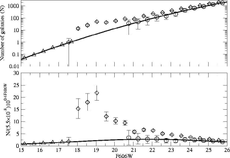
Figure 5: Top panel Galaxy number counts as a function of F606W magnitude for Abell 2218 (diamonds), the combined HDF-North, HDF-South and WFPC2 counts (open circles) and the MGC counts (triangles). The solid line is a polynomial fit to all the reference field counts. Bottom panel The galaxy number counts shown relative to the $N\propto 10^{0.4\,m}$ relation.

Table 1 provides a tabulation of the galaxy counts (and their associated errors) relevant to our A2218 analysis. In column 2 we list the total counts, $n_{tot}$, observed within our A2218 field and in column 5 our estimates of the numbers of field galaxies, $n_{ref}$, within the A2218 mosaic field-of-view, based on the above quadratic fit. Columns 3 and 6 give estimates for the Poisson noise in the components that make up each observed count: the standard deviation of the counts along the cluster line of sight:

$$P_{\rm tot}=\sqrt{n_{tot}},$$ (2)

and the error due to Poisson noise in our estimate of the mean field (or reference) count:

$$P_{\rm ref}=\sqrt{{\Omega_{\rm A2218}\over\Omega_{\rm WFPC2}}{n_{ref}\over 12}},$$ (3)

respectively. Here $\Omega_{\rm A2218}$ and $\Omega_{\rm WFPC2}$ represent the area of sky covered by our A2218 observations and within one WFPC2 field, respectively.

There is an additional uncertainty in the galaxy counts as a result of general galaxy clustering along the line of sight to A2218 (Glazebrook et al. 1994, Djorgovski et al. 1995). The error introduced by this effect has been computed by Huang et al. (1997) and is given by their equations 5 and 6. An analogous formula is also given by Driver et al. (2003; equation 7). This is a vital component which typically dominates the error budget at faint magnitudes and has often been neglected in previous studies. The errors introduced into our counts by general galaxy clustering along the line of sight to the A2218 field ($C_{\rm c}$) and to the reference fields ($C_{\rm ref}$) are given in columns 4 and 7, respectively. They have been calculated using the Driver et al. equation:

$$\epsilon^{2}(N)=({\sqrt{2}\over 3})^{-0.8}\cdot\Omega^{-0.4}\cdot N^{2}(m)\cdot{10^{-0.235m+2.73}}.$$ (4)

Here, $N$ is the field number counts (per 0.5 mag interval) and $\Omega$ is the area of sky over which the counts are measured. The field galaxy counts appropriate to our A2218 field (and hence to the derivation of the ‘clustering’ errors listed in column 4) are given in column 5 of Table 1. These have been derived using the above quadratic representation of the MGC+WFPC2 counts, with the appropriate normalisation applied to account for the different sky coverage: $\Omega_{\rm A2218}=0.0228$ sq. deg, $\Omega_{\rm MGC}=30.310$ sq. deg, $\Omega_{\rm WFPC2}=0.0011$ sq. deg. The small area of the WFPC2 field means that the counts observed within it are more susceptible to line-of-sight clustering, as can be seen in the larger ‘clustering’ errors listed for the field in column 7 of Table 1.

In Figure 6 we show how the observed variance in the galaxy number counts from field to field compares with what we would expect based on our above error budget analysis. It can be seen that, overall, there is good agreement between the two, with our predictions, if anything, being slightly pessimistic.

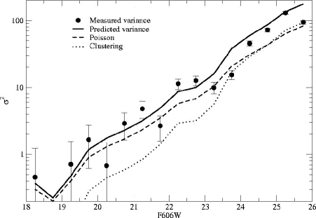
Figure 6: Comparison of the measured variance in the 12 reference fields (filled circles) and the predicted variance as described in the text (solid line). The dashed line and dotted line show the Poisson and clustering contributions to the predicted variance respectively. Note that the error bars plotted for the observed points were determined using a ‘jack-knife’ method.

The final column of Table 1 contains the field-subtracted ‘cluster’ counts within our A2218 field, with their quoted uncertainties representing the combination of all the contributing errors described above. Figure 7 shows graphically the contribution of each of the four errors to the final error budget.

$F606W$	$n_{tot}$	$P_{tot}$	$C_{\rm c}$	$n_{ref}$	$P_{\rm ref}$	$C_{\rm ref}$	$n_{clus}(n_{tot}-n_{ref})$
17.55	1	1	0.53	0.92	1.23	0.27	$0.1\pm 1.7$
18.05	14	3.74	0.82	1.63	1.64	0.42	$12.4\pm 4.2$
18.55	26	5.10	1.26	2.87	2.18	0.65	$23.1\pm 5.7$
19.05	50	7.07	1.91	4.97	2.86	0.98	$45.0\pm 7.9$
19.55	43	6.56	2.85	8.47	3.74	1.46	$34.5\pm 8.2$
20.05	59	7.68	4.18	14.23	4.85	2.14	$44.8\pm 10.2$
20.55	86	9.27	6.05	23.57	6.24	3.10	$62.4\pm 13.1$
21.05	83	9.11	8.62	38.46	7.97	4.42	$44.5\pm 15.5$
21.55	151	12.29	12.11	61.82	10.11	6.20	$89.2\pm 20.9$
22.05	229	15.13	16.75	97.92	12.72	8.58	$131.1\pm 27.3$
22.55	288	16.97	22.84	152.82	15.89	11.70	$135.2\pm 34.6$
23.05	414	20.35	30.67	234.99	19.70	15.71	$179.0\pm 44.6$
23.55	594	24.37	40.59	356.01	24.25	20.79	$238.0\pm 57.1$
24.05	812	28.50	52.92	531.42	29.63	27.10	$280.6\pm 72.3$
24.55	1089	33.00	67.99	781.60	35.93	34.82	$307.4\pm 90.6$
25.05	1539	39.23	86.05	1132.64	43.25	44.07	$406.4\pm 113.0$
25.55	2044	45.21	107.32	1617.20	51.68	54.97	$426.8\pm 138.8$

Table 1: Summary of the number counts for A2218. The total galaxy counts detected in the A2218 field (column 2) and the field reference counts (column 5) along with all the associated errors (see text). The final column gives the field subtracted galaxy counts along with the combined error.

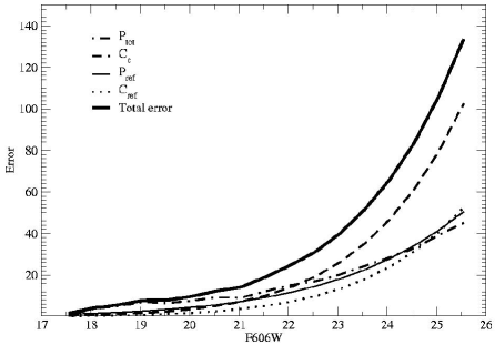
Figure 7: The errors in the Abell 2218 number counts as a function of magnitude. The four individual error components are shown along with the combined total error (solid line).

2.3 Lensing

A further possible correction to the background counts concerns the effects of gravitational lensing of the background population by the cluster mass (Trentham 1998). This consists of two competing effects: a magnification effect, where the background population is brightened and therefore seen in greater numbers at any given magnitude, and an apparent expansion of the background field behind the cluster, which reduces the surface density of background objects. The precise details of the combined correction required to account for these two effects are given in Bernstein et al. (1995) and Trentham (1998); we therefore give here only a brief outline of the model which we will use to estimate the effect of lensing in A2218.

The quantity that requires computation is the fractional change in the counts due to lensing:

$$f_{\rm lens}={N^{\prime}(m)\over N(m)},$$ (5)

where $N(m)$ is the observed reference counts per unit area and $N^{\prime}(m)$ is the counts we should instead observe when the lensing effect of the cluster is taken into account. Calculation of $N^{\prime}(m)$ requires knowledge of the number of galaxies per unit redshift per magnitude per steradian, which is given by:

$$n(m,z)={\ln(10)\over 10\pi}\phi(m,z){dV\over dz},$$ (6)

where $\phi(m,z)$ is the field galaxy luminosity function at redshift $z$. We assume that this can be described by a Schechter function at all redshifts, with luminosity evolution parameterized by:

$$\phi^{*}(z)=\phi^{*}(0)(1+z)^{2}$$ (7)

$$M^{*}(z)=M^{*}(0)+5\log(1+z)$$ (8)

(see Broadhurst et al. 1995, Trentham 1998). We use the local luminosity function measured from the 2dF Galaxy Redshift Survey (Norberg et al. 2001) and the colour transformations from Driver et al. (2003) which, after conversion to our cosmology, results in $\phi^{*}=0.0169{\rm Mpc}^{-3}$, $M^{*}=-20.65$ and $\alpha=-1.21$. The volume element is given by:

$${dV\over dz}=\Omega x^{2}{dx\over dz},$$ (9)

where $x$ is the comoving distance, and for a flat cosmology:

$${dx\over dz}={c\over H_{0}\sqrt{\Omega_{m}(1+z)^{3}+\Omega_{\Lambda}}}.$$ (10)

Having defined the model $n(m,z)$ distribution, the true $N(m,z)$ can be recovered by requiring that ${\int_{0}}^{\infty}N(m,z)dz$ reproduces the observed number counts, that is:

$$N(m,z)={N(m)\over{\int_{0}}^{\infty}n(m,z)dz}n(m,z).$$ (11)

The function $N^{\prime}(m)$ is then given by:

$$N^{\prime}(m,z)={1\over A}N(m+2.5\log A,z),$$ (12)

where $A$ is the amplification of the lens. Again, following Trentham, we assume the cluster mass profile to be a spherically symmetric isothermal sphere. $A$ is then given by:

$$A(r,z)=\left|{1-{4\pi\sigma^{2}D_{c}D_{cs}(z)\over rc^{2}D_{s}(z)}}\right|^{-1}$$ (13)

where $D_{c}$, $D_{s}$ and $D_{cs}$ are the angular diameter distances to the cluster, to the source and from the cluster to the source respectively (Miralda-Escude 1991). $f_{lens}$ can then be calculated by radially averaging ${N^{\prime}\over N}$ over the annulus for which we want to evaluate the lensing correction:

$$f_{lens}(m)={2\int_{r_{1}}^{r_{2}}\left[\int_{0}^{z_{c}}N(m,z)dz+\int_{z_{c}}^{\infty}N^{\prime}(m,z,r)dz\right]rdr\over r_{2}^{2}-r_{1}^{2}},$$ (14)

where $r_{1}$ and $r_{2}$ are the inner and outer radii of the annulus.

In Figure 8 we plot $f_{\rm lens}$ for a series of annuli in which we will derive cluster LFs in our subsequent analysis. The solid line shows $f_{\rm lens}$ for the inner region of the cluster bounded by $r_{1}=100$ kpc and $r_{2}=300$ kpc. It is this region where the effects of lensing are at their maximum. Note that the inner 100 kpc has been excluded due to the unrealistic nature of the isothermal model in that region (AbdelSalam, Saha & Williams 1998). The dotted line shows $f_{\rm lens}$ for the outer region of the cluster, with boundaries $r_{1}=300{\rm kpc}$ and $r_{2}=750{\rm kpc}$. Finally, the dashed line shows $f_{\rm lens}$ for an annulus encompassing the ‘whole’ field: $r_{1}=100{\rm kpc}$ to $r_{2}=750{\rm kpc}$.

In general, the family of curves shown in Figure 8 are in excellent agreement with those derived by Trentham (for Abell 665 at $z=0.18$; see his Figure 3) in terms of their overall behavior with apparent magnitude, the amplitude of the effect ($\mathrel{\raise 1.50696pt\hbox{$\scriptstyle<$}\kern-6.00006pt\lower 1.72218pt\hbox{{$\scriptstyle\sim$}}}10\%$), and its much diminished importance at larger clustercentric radii. The only systematic difference of note is that our $f_{\rm lens}$ function drops below unity at faint magnitudes ($F606W>23$) – that is, lensing decreases (rather than boosts) the number of faint background galaxies seen in the direction of the cluster. This difference can be attributed to slightly different assumptions made about the $n(m,z)$ distribution, in particular the differences in the representations of the observed galaxy counts, $N(m)$, in normalizing $n(m,z)$. Here Trentham uses a linear function to represent $d\log N/dm$, whereas we have used a quadratic representation (see Figure 5).

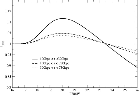
Figure 8: The function $f_{\rm lens}$, averaged over three different annuli: $100{\rm kpc}<r<300{\rm kpc}$ (solid line), $100{\rm kpc}<r<750{\rm kpc}$ (dashed line) and $300{\rm kpc}<r<750{\rm kpc}$ (dotted line).

3 Results

3.1 Luminosity Function

As a first step in our analysis, we take the final field-corrected cluster counts listed in the final column of Table 1 and construct the luminosity distribution (LD) for A2218’s galaxy population; this is shown in Figure 9 (filled circles). Formally, this distribution is well described by a Schechter function with $M^{*}_{\rm F606W}=-20.52\pm 0.27$ and $\alpha=-1.38\pm 0.05$ over the range $-21.5<M_{\rm F606W}<-13.2$ (solid line in left panel of Figure 9). Because the errors in $M^{*}$ and $\alpha$ are tightly correlated, we present alongside our derived LD the error contours for these two parameters (the thick lines in the right-hand panel). Also shown in this figure is the LD recovered after the reference field counts have been scaled by $f_{\rm lens}$ (dashed line in Figure 8) to correct for lensing effects (open circles). It can be seen that this makes very little difference to our observed LD. This is reflected quantitatively in the values of the fitted Schechter function parameters, $M^{*}_{\rm F606W}=-20.25\pm 0.28$ and $\alpha=-1.40\pm 0.05$, which differ from the original values by less than $1\sigma$.

For comparison, we also plot in Figure 9 the $M^{*}_{\rm F606W}$ and $\alpha$ values for the Schechter function fits to the composite LF derived for the $z\sim 0.1$ clusters in the 2dF Galaxy Redshift Survey (2dFGRS; De Propris et al. 2003), and the LF derived for the rich cluster Abell 868 ($z=0.15$) from a comparable HST-based dataset to what we have used here, by Driver et al. (2003). It can be seen that our A2218 LF has a steeper faint-end slope (more negative value of $\alpha$) and a slightly fainter $M^{*}$ than these other two LFs, particularly for the 2dFGRS clusters where, given the size of the error bars, the differences are reasonably significant. On the other hand, the 2dFGRS and A868 LFs do not extend as faint as ours ($M_{\rm F606W}\simeq-16$ cf. $M_{\rm F606W}\simeq-13$), and it is well known that the value of the parameter $\alpha$ is quite sensitive to the luminosity range covered, with the faint end steeping at fainter magnitudes (Lobo et al. 1997). A better comparison is obtained by fitting the A2218 data over the same absolute magnitude range, for which we recover $M^{*}_{\rm F606W}=-20.26\pm 0.27$ and $\alpha=-1.23\pm 0.09$. This is also the range over which our sample is complete with respect to surface brightness. The error contours for the LF parameters fit over this range are shown as the thin contours in Figure 9. We see that the LF in this case has a shallower slope, with its $\alpha$ value being consistent with those of the 2dFGRS and A868 LFs. However, the small offset in $M^{*}$ still remains. Such small differences may well result from the regions of the clusters being compared here not being identical; the likelihood of this being the case is highlighted below.

Finally, it is also worth noting that we see evidence of an ‘inflexion’ in A2218’s LF at $M_{\rm F606W}\approx-18$, something which has been seen in many other clusters (e.g. Driver et al. 1998a; Barkhouse, Yee & Lopez-Cruz 2002).

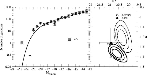
Figure 9: Left panel: The galaxy luminosity distribution derived for A2218. The data are represented by circles; those that are filled have had no correction for the effects of gravitational lensing, whereas the open circles include this correction. The data point contributed by the central cD galaxy is shown as the filled square. A Schechter function fit to the (uncorrected) data points is represented by the solid line. Right panel: The $1\sigma$, $2\sigma$ and $3\sigma$ error contours for the Schechter function parameters $M^{*}$ and $\alpha$ for $M<-13.2$ (thick contours) and $M<-16$ (thin contours) . For comparison, the values of these parameters for the 2dFGRS composite cluster LF (De Propris et al. 2003) and that of A868 (Driver et al. 2003) are represented by the open and filled circles, respectively.

The wide field provided by the 22 WFPC2 pointings allows us to sub-divide the cluster into projected ‘core’ and ‘halo’ components and re-derive the luminosity distributions for each component. To do this we split the inner and outer regions at $300h^{-1}$ kpc from the central, dominant cD galaxy. Somewhat arbitrarily, this radius was chosen to be twice the typical cluster core radius, as measured, for example, for the ENACS sample (Adami et al. 1998). In assembling the luminosity distribution for the inner region, we exclude the central $100h^{-1}$ kpc because of our inability to compute lensing corrections in this region (see Section 2.3). The outer radial limit is $\approx 750h^{-1}$ kpc.

Figure 10 shows the resulting LDs with both the uncorrected (solid symbols) and lensing corrected (open symbols) data points plotted. Our Schechter function fits and error-contours are shown in the usual way; because the lensing corrections have a negligible effect, only those based on the uncorrected data are displayed. From Figure 10 we see that the LD for the central region has a significantly flatter faint-end slope than that for the outer region. The inner ‘core’ LF has a slope of $\alpha=-1.23\pm 0.13$ while the outer ‘halo’ LF has $\alpha=-1.49\pm 0.06$. This is in line with recent claims that the LF of galaxies in the Coma cluster is flatter in the vicinity of the two central dominant giants, with it steepening as a function of clustercentric distance (Beijersbergen et al. 2002; see also Lobo et al. 1997). Driver et al. (2003) obtained a a similar result from their LF analysis of A868. Barkhouse et al. (2002) also find a significant steepening of the LF as a function of clustercentric radius in their sample of local clusters as do Sabatini et al. (2003) for the Virgo cluster and Andreon (2002) for the $z=0.31$ cluster A2744. Similarly, luminosity segregation may be responsible for the dwarf population density relation discussed in the following two sections. However, Mobasher et al. (2003) argue against the claim of Beijersbergen et al. (2002) for luminosity segregation in Coma, while Paolillo et al. (2001) fail to find steeper LFs in their composite LF for the outer regions of nearby clusters.

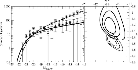
Figure 10: Left panel: Galaxy luminosity distributions (LDs) for A2218, split on the basis of clustercentric radius. The LD for galaxies in the inner ‘core’ region of the cluster ($100\leq r<300$ kpc) is represented by circles; those that are filled have had no correction for the effects of gravitational lensing, whereas the open circles include this correction. The LD for galaxies in the outer ‘halo’ region of the cluster ($300\leq r<750$ kpc) is represented by squares, differentiated in the same way to show the effects of lensing corrections. Shechter function fits to the uncorrected data are shown as the thick and thin solid lines for the inner and outer regions, respectively. Right panel: The $1\sigma$, $2\sigma$ and $3\sigma$ error ellipses for the Schechter function parameters, $M^{*}_{\rm F606W}$ (horizontal axis) and $\alpha$ (vertical axis), derived from the fits shown in the left-hand panel; inner region (thick lines), outer region (thin lines).

3.2 Dwarf-to-giant ratio

A simpler, non-parametric method to test for the luminosity segregation indicated in Figure 10, is to measure the dwarf-to-giant ratio (DGR – Driver et al. 1998a). This is much less sensitive to the correlated errors that affect the Schechter LF parameters. To do so, we define ‘giants’ as galaxies brighter than $M_{\rm F606W}=-18$ and ‘dwarfs’ as galaxies with $-18<M_{\rm F606W}<-15$. The DGR – the ratio of the numbers of so defined dwarfs to giants – was calculated for each dwarf galaxy by finding the distance to its 10th nearest giant galaxy and counting the number of dwarf galaxies within the same region. The area of the circle was calculated numerically to take into account gaps in the mosaic (Figure 1). The local galaxy density (Dressler 1980) was then simply taken as 10 divided by this area. In order to reduce errors, the data were then binned according to the local giant galaxy density measured in the vicinity of each dwarf galaxy. Field subtraction was performed using the smoothed counts from Figure 5.

Figure 11 shows the DGR plotted as a function of local giant galaxy density. Our results show clearly that the DGR in A2218 decreases smoothly and monotonically with increasing local giant galaxy density, consistent with the dwarf population–density relation proposed by Phillipps et al. (1998). Indeed our data define the relation much more cleanly and over a large range in galaxy density than the data from Smith et al. (1997) and Driver et al. (1998a) (which we also plot in Figure 11 for a qualitative comparison) upon which Phillipps et al’s proposed relation was based. That these latter data points all appear to sit lower on the diagram with respect to our A2218 data is most likely attributable to differences in filters, magnitude depths and binning in galaxy density between the different studies.

Our data are of sufficient depth to allow us to also consider a fainter sample of ‘ultra-dwarf’ galaxies, with $-13.5<M_{\rm F606W}<-15$. The DGR values for this population are also plotted in Figure 11 and appear to follow the same trend with density as the brighter sample, indicating commonality between the ultra-dwarf and dwarf populations.

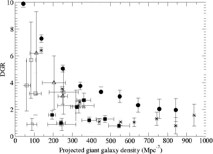
Figure 11: The variation of the dwarf-to-giant galaxy ratio (DGR) with local giant galaxy density. Filled circles represent the ‘intermediate’ dwarfs ($-18<M_{\rm F606W}<-15$) in A2218; starred points represent the ‘ultra-dwarfs’ ($-15<M_{\rm F606W}<-13.5$) in A2218. The error bars include Poisson contributions only and lensing effects are ignored. The open triangles show the data for A2554 from Smith et al. (1997). The filled squares represent the central regions of the clusters from Driver et al. (1998a) and the open squares the outer regions.

3.3 The radial profile of galaxies in A2218

In order to determine whether or not the decreasing DGR is due only to the increasing giant galaxy density toward the cluster core or whether there is a corresponding decrease in the number of dwarfs for higher giant galaxy densities, we have derived radial density profiles for these different sub-populations within A2218. These are plotted in Figure 12, with the data for the giants ($M_{\rm F606W}<-18$) shown in the top panel, those for the ‘intermediate’ dwarfs ($-18<M_{\rm F606W}<-15$) shown in the middle panel, and those for the ‘ultra-dwarfs’ ($-15<M_{\rm F606W}<-13.5$) shown in the bottom panel. Again the data with and without corrections for lensing are plotted, and it can be that the difference between them is negligible. Accordingly, in fitting the data with a power-law ($\sigma(r)\propto r^{a}$; solid lines in Fig. 12), we do so to the uncorrected data only. Note that we also exclude the innermost radial point in these fits as well (corresponding to the inner $100h^{-1}$ kpc where the lensing correction is uncertain.

The giant galaxy projected density is seen to drop off with a power-law index $a=-1.13\pm 0.15$, consistent with that of a projected isothermal sphere ($\propto a^{-1}$). We also note that beyond a radius of $\sim 1$ arcmin ($\sim 128$ kpc), it traces very well the projected X-ray gas density profile (dashed line) observed for A2218 (Machacek et al. 2002), which has a core radius of $r_{\rm c}=66.4^{\prime\prime}$ and $\beta=0.705$.

For the intermediate luminosity dwarfs, the distribution is flatter than that of the giants and is best fit by a power-law with index $a=-0.63\pm 0.09$. In contrast, the ultra-dwarf galaxy surface density shows a deficiency in the centre of the cluster, and then is approximately flat at $r>0.6$ arcmin ($\sim 200\,h^{-1}$ kpc). A power-law fit to the data has a index of $a=-0.03\pm 0.13$. The most likely explanation for this behavior is that the fainter galaxies have a more extended distribution, and hence larger scale radius, than the giants, as also seen for the bright and faint dEs in the Coma cluster (Secker et al. 1997).

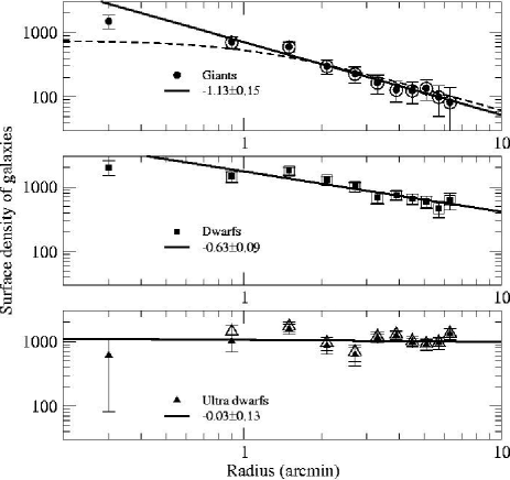
Figure 12: Radial surface density distributions for the giant, dwarf, and ultra-dwarf galaxy populations in A2218: Top panel: the giant ($M_{\rm F606W}<-18$) galaxies, with the uncorrected data shown as filled circles, and the lensing-corrected data shown as open circles. The projected X-ray gas density profile is shown as the dashed line. Middle panel: the intermediate dwarf ($-18<M_{\rm F606W}<-15$) galaxies, with the uncorrected data shown as filled squares and the lensing-corrected data shown as open squares. Bottom panel: the ultra-dwarf ($-15<M_{\rm F606W}<-13.5$) galaxies, with the uncorrected data shown as filled triangles and the lensing-corrected data shown as open triangles. A power-law fit to the uncorrected data points is represented in all three panels by the solid line.

There are two competing effects which should be considered in interpreting Figure 12. Firstly, because of the larger galaxy density in the centre of the cluster there is a diminishing area effect where the field of view in which dwarf galaxies can be detected is reduced due to the presence of brighter galaxies (see Driver et al. 1998b). To determine the extent of this effect, we sum together the areas assigned to detected objects by SExtractor in both the very central region of the cluster and in the lowest density regions. We find in the central region the total area associated with objects by SExtractor is 8.2% of the total area, while in the outskirts only 4.2% of the area is occupied by objects. Hence if the data in Figure 12 were to be corrected for this effect, it would amount to only a 4% differential adjustment between the innermost (highest density) and outermost (lowest density) bins. This would have a negligible effect in terms of the overall trends seen in the bottom two panels.

Secondly, there is a radial dependence on the volume of cluster sampled per unit area projected on the sky. Assuming the cluster fills a sphere of radius $R$, then the volume per unit area projected onto a circle of radius $a$ centered on the cluster is :

$${{\rm Volume}\over{\rm Area}}\approx{4\over 3a^{2}}(R^{3}-(R^{2}-a^{2})^{3\over 2}).$$ (15)

Hence the volume per unit area decreases with radius. If we assume a physical radius for A2218, then we can calculate the corrections in number needed in each of the radial bins in Figure 12. For a spherical cluster with a $1.5\,h^{-1}$ Mpc radius (approximately the Abell radius), a factor of 1.15 increase in number is required in the outermost annuli (with respect to the innermost annuli) to convert from number per unit area to number per unit volume. This more than compensates for the correction (in the opposite sense) due to the diminishing area effect. So it is likely that the differences in profile shape for the giant, dwarf, and ultra-dwarf galaxy populations are as large, if not larger than that seen in Figure 12, and the flattening of profile shape with decreasing luminosity is a real effect, when both these effects are taken into account.

4 Summary and discussion

We have exploited deep, wide-field HST imagery of the well known rich cluster A2218 at $z=0.18$, to conduct a census of its galaxy population over a $\sim 10$ magnitude range in luminosity ($-23<M_{\rm F606W}<-13$), and thereby explore how its constituent ‘giant’ and ‘dwarf’ galaxy populations vary in number as a function of location and environment within the cluster.

Taking the complete ensemble of A2218 galaxies that are identified, statistically, within the entire central 1.34 Mpc² $h^{-2}$ field studied and over the full range in luminosity and surface brightness ($\mu_{F606W}\mathrel{\raise 1.50696pt\hbox{$\scriptstyle<$}\kern-6.00006pt\lower 1.72218pt\hbox{{$\scriptstyle\sim$}}}24.7$ mag arcsec^-2) probed, we find their luminosity distribution to be well fitted by a Schechter function, with parameters $M_{\rm F606W}^{*}=-20.52\pm 0.27$ and $\alpha=-1.38\pm 0.05$. In terms of the faint-end slope, at least, this is in reasonable agreement with the LFs measured for other rich clusters, both at similar and more nearby redshifts.

Importantly, however, our study has also revealed that such ‘global’ measures of the LF represent the superposition of a number of important underlying dependencies on clustercentric radius and, more fundamentally, the local galaxy density. The most conspicuous of these is a change in the shape of A2218’s LF with clustercentric radius, in particular its faint end having a steeper slope at larger radii. This indicates that the relative balance between the numbers of dwarf and giant galaxies varies with environment in the cluster, and we have quantified this by measuring the ratio of dwarf to giant galaxies (DGR) as a function of local projected galaxy density. We find the DGR in A2218 to decrease monotonically with increasing local density, dropping by an order of magnitude (from $\sim 10$ to $\sim 1$) in going from the lowest ($\sim 100$ gals Mpc^-2) to the highest ($\sim 1000$ gals Mpc^-2) densities probed by our observations. This confirms the existence of a “dwarf galaxy–density relation” as first suggested by Phillipps et al. (1998). Furthermore, we have shown that this relation arises from galaxies of different luminosity having quite different radial surface density profiles. The brightest, giant galaxies have the steepest profile, consistent with an isothermal sphere and that of the hot X-ray gas. The fainter, dwarf galaxies have much shallower profiles, indicating that they are a much more extended population with a much larger scale radius. Indeed the ‘ultra-dwarf’ galaxy population in A2218 is found to have a radial profile which is essentially flat, indicating a constant surface density at least over the central 750 kpc studied here.

This quite clear ‘segregation’ between galaxies in these different luminosity regimes could be a result of primordial conditions, evolution, or both. As has been previously discussed by Phillipps et al. (1998), the numerical CDM models of Kauffmann et al. (1997) point to the dwarf population–density relation being a natural consequence of the hierarchical clustering process. In this picture the dwarf galaxies, which form via the gravitational collapse of small amplitude density peaks in the primordial universe, are predicted to be more numerous and less clustered than their brighter counterparts.

However, Moore et al. (1998) have also been able to explain the dwarf population–density relation as the result of galaxy ‘harassment’, which operates more effectively in denser regions. As the cluster tidal field becomes increasingly important in the cluster centre, the smaller spheroidal galaxies will be destroyed in the innermost part of the cluster and global tides will disintegrate the lowest surface brightness objects into the diffuse stellar background. In the Coma cluster, for example, Biviano et al. (1996) find that the cluster structure is better traced by the faint galaxy population, which forms a single smooth structure, with the brighter galaxies being located in sub-clusters. They interpreted this as evidence for the ongoing accretion of groups onto the main body of the cluster. In this context, it is interesting to note that Bernstein et al. (1995) find a significant flattening of the density profile of faint galaxies in the inner 100 kpc of the Coma cluster.

The deficiency of dwarf galaxies in the centre of Abell 2218 may also be related to the presence of a cD galaxy. cD galaxies probably form suddenly during the collapse and virialization of compact groups or poor clusters which then merge with other groups to form a rich cluster (Merritt 1985). Lopez-Cruz et al. (1997) suggest that the flatter faint-end slope of the galaxy LF which they find in rich clusters, in particular clusters that contain cD galaxies, results from the disruption of large number of dwarf galaxies early on in the clusters evolution. A similar effect is claimed by Barkhouse et al. (2002). The stars from the disrupted galaxies are redistributed throughout the cluster, generating the cD halo. This is consistent with a lack of dwarf galaxies in the core of Abell 2218.

Ultimately, a single cluster is not sufficient to both establish the trends we discussed and analyse their dependence on cluster properties. A larger sample of clusters with deep, wide-field imaging is needed to make progress on these important issues. This is a project we are currently embarking upon, the results from which will be reported in future papers.

References

- [AbdelSalam, Saha & Williams (1998)] AbdelSalam, H.M., Saha, P., Williams, L.L.R. 1998, ApJ, 116, 1541
- [Adami et al.(1998)] Adami C., Mazure A., Katgert P., Biviano A. 1998, A&A, 336, 63
- [Andreon(2002)] Andreon S. 2002, A&A, 382, 821
- [Barkhouse et al.(2002)] Barkhouse W. A., Yee H. K. C., Lopez-Cruz O. 2002, in Tracing Cosmic Evolution with Galaxy Clusters, ASP Conference Proceedings 268, ed. S. Borgani, M. Mezzetti, R. Valdarnini (San Francisco: Astronomical Society of the Pacific), p. 289
- [Bekki et al.(2001)] Bekki K., Couch W. J., Shioya Y., 2001, PASJ, 53, 395
- [Beijersbergen et al.(2002)] Beijersbergen M., Hoekstra H., van Dokkum P. G., van der Hulst T. 2002, MNRAS, 329, 385
- [Benson et al.(2003)] Benson, A., Bower, R.G., Frenk, C., Lacey, C.G., Baugh, C.M., Cole, S., 2003, ApJ, 599, 38
- [Bernstein et al.(1995)] Bernstein G. M., Nichol R. C., Tyson J. A., Ulmer M. P., Wittman D., 1995, AJ, 110, 1507
- [Bertin & Arnouts(1996)] Bertin E., Arnouts S., 1996, A&AS, 117, 393
- [Binggeli et al.(1985)] Binggeli B., Sandage, A., Tammann G. A., 1985, AJ, 90, 1681
- [Binggeli et al.(1988)] Binggeli B., Sandage, A., Tammann G. A., 1988, ARA&A, 26, 509
- [Birkinshaw & Hughes(1994)] Birkinshaw, M., Highes, J.P., 1994, ApJ, 420, 33
- [Biviano et al.(1996)] Biviano A., Durret F., Gerbal D., Le Fevre O., Lobo C., Mazure A. & Slezak E., 1996, A&A, 311, 95
- [Bower & Balogh(2003)] Bower, R.G., Balogh, M.L., 2003, in Clusters of Galaxies: Probes of Cosmic Structure and Evolution, ed. J.S. Mulchaey, A. Dressler, A. Oemler, (Cambridge: Cambridge Univ. Press), in press
- [Broadhurst et al.(1995)] Broadhurst T. J., Taylor A. N., Peacock J. A., 1995, ApJ, 438, 49
- [Byrd & Valtonen(1990)] Byrd G. G., Valtonen M. J., 1990, ApJ, 350, 89
- [Casertano et al.(2000)] Casertano S. et al. 2000, AJ, 120, 2747
- [Conselice et al.(2003)] Conselice C., O’Neil K., Gallagher J.S., Wyse R.F.G., 2003, ApJ, 591, 167
- [De Propris & Pritchet(1998)] De Propris R., Pritchet C. J. 1998, AJ, 116, 1118
- [De Propris et al.(2003)] De Propris R. et al. 2003, MNRAS, 342, 725
- [Djorgovski et al.(1995)] Djorgovski S., et al. 1995, ApJ, 438, L13
- [Dressler(1980)] Dressler, A. 1980, ApJ, 236, 351
- [Driver et al.(1998a)] Driver S. P., Couch W. J., Phillipps S. 1998a, MNRAS, 301, 369
- [Driver et al.(1998b)] Driver S.P., Couch W.J., Phillipps S., Smith R.M., 1998b, MNRAS, 301, 357
- [Driver et al.(2003)] Driver S. P., Odewahn S. C., Echevarria L., Cohen S. C., Windhorst R. A., Phillipps S., Couch W. J., 2003, AJ, 126, 2662
- [Driver & De Propris(2003)] Driver S. P., De Propris R. 2003, Ap&SS, 285, 175
- [Glazebrook et al.(1994)] Glazebrook K., Peacock J. A., Collins C. A., Miller L., 1994, MNRAS, 266, 65
- [Gunn & Gott(1972)] Gunn J. E., Gott J. R., 1972, ApJ, 176,1
- [Holtzman et al.(1995)] Holtzman J. A., Burrows C. J., Casertano S., Hester J. J., Trauger J. T., Watson A. M., Worthey G., 1995, PASP, 107, 1065
- [Huang et al.(1997)] Huang J. S., Cowie L. L., Gardner J. P., Hu E. M., Songaila A., Wainscoat R. J., 1997, ApJ, 476, 12
- [Jones et al.1993] Jones, M., et al., 1993, Nature, 365, 320
- [Kauffmann et al.(1993)] Kauffmann G., White S. D. M., Guiderdoni B., 1993, MNRAS, 264, 201
- [Kauffmann et al.(1997)] Kauffmann G., Nusser A., Steinmetz M., 1997, MNRAS, 286, 795
- [Kneib et al.(1996)] Kneib J. P., Ellis, R.S., Smail, I., Couch, W.J., Sharples, R.M., 1996, ApJ, 471, 643
- [Kneib et al.(1995)] Kneib J. P., Mellier Y., Pello R., Miralda-Escude J., Le Borgne J. F., Böhringer H., Picat J. P., 1995, A&A, 303, 27
- [Koekemoer et al.(2002)] Koekemoer A. et al. 2002, HST Dither Handbook version 2.0 (Baltimore: STScI)
- [Kron(1980)] Kron R. G., 1980, ApJS, 43, 305
- [Le Borgne et al.(1992)] Le Borgne J. F., Pello R., Sanahuja B., 1992, A&AS, 130, 65
- [Liske et al.(2003)] Liske J., Lemon D. J., Driver S. P., Cross N. J. G. & Couch W. J., 2003, MNRAS, 344, 307
- [Lobo et al.(1997)] Lobo C., Biviano A., Durret F., Gerbal D., Le Fevre O., Mazure A., Slezak E., 1997, A&A, 317, 385
- [Lopez-Cruz et al.(1997)] Lopez-Cruz O., Yee H. K. C., Brown J. P., Jones C., Forman W., 1997, ApJ, 475, L97
- [Machacek et al.(2002)] Machacek M. E., Bautz M. W., Canizares C., Garmire G. P., 2002, ApJ, 567, 188
- [Metcalfe et al.(2001)] Metcalfe, N., Shanks, T., Campos, A., McCracken, H.J., Fong, R., 2001, MNRAS, 323, 795
- [Merritt(1985)] Merritt D., 1985, ApJ, 289, 18
- [Miralda-Escude(1991)] Miralda-Escude J., 1991, ApJ, 370, 1
- [Mobasher et al.(2003)] Mobasher, B., Colless M., Carter D., Poggianti B. M., Bridges T. J., Kranz K., Kominyama Y., Kashikawa N., Yagi M., Okamura S., 2003, ApJ, 587, 605
- [Moore et al.(1996)] Moore B., Katz N., Lake G., Dressler A., Oemler A. 1996, Nature, 379, 613
- [Moore et al.(1998)] Moore B., Lake G., Katz N., 1998, ApJ, 495, 139
- [Moore(2003)] Moore B. 2003, in Clusters of Galaxies: Probes of Cosmic Structure and Evolution, ed. J.S. Mulchaey, A. Dressler, A. Oemler, (Cambridge: Cambridge Univ. Press), in press
- [Norberg et al.(2002)] Norberg, P., et al., 2002, MNRAS, 336, 907
- [Paolillo et al.(2001)] Paolillo M., Andreon S., Longo G., Puddu E., Gal R. R., Scaramella R., Djorgovski S. G., de Carvalho R., 2001, A&A, 367, 59
- [Pello-Descayre et al.(1988)] Pello-Descayre R., Sanahuja B., Soucail G., Mathez G., Ojero E., 1988, A&A, 190, L11
- [Phillipps et al.(1998)] Phillipps S., Driver S. P., Couch W. J., Smith R. M., 1998, ApJ, 498, L119
- [Press & Schechter(1974)] Press W. H., Schechter P. 1974, ApJ, 187, 425
- [Sabatini et al.(2003)] Sabatini S., Davies, J.I., Scaramella R., Smith R.M., Baes M., Linder S.M., Roberts S., Testa V., 2003, MNRAS, 341, 981
- [Schechter(1976)] Schechter P. 1976, ApJ, 203, 297
- [Secker et al.(1997)] Secker J., Harris W. E., Plummer J. D., 1997, PASP, 109, 1377
- [Smith et al.(1997)] Smith R. M., Driver S. P., Phillipps S., 1997, MNRAS, 287, 415
- [Trentham(1998)] Trentham N. 1998, MNRAS, 295, 360
- [Trentham N. & Tully(2002)] Trentham N., Tully R. B. 2002, MNRAS, 335, 712
- [White & Rees(1978)] White S.D.M., Rees, M., 1978, MNRAS, 183, 341
- [Williams et al.(1996)] Williams R. E. et al. 1996, AJ, 112, 1335